Abstract
The state of health (SOH) evaluation and remaining useful life (RUL) prediction for lithium-ion batteries (LIBs) are crucial for health management. This paper proposes a novel sequence-to-sequence (Seq2Seq) prediction method for LIB capacity degradation based on the gated recurrent unit (GRU) neural network with the attention mechanism. An improved particle swarm optimization (IPSO) algorithm is developed for automatic hyperparameter search of the Seq2Seq model, which speeds up parameter convergence and avoids getting stuck in local optima. Before model training, the complete ensemble empirical mode decomposition with adaptive noise (CEEMDAN) algorithm decomposes the capacity degradation sequences. And the intrinsic mode function (IMF) components with the highest correlation are employed to reconstruct the sequences, reducing the influence of noise in the original data. A real-cycle-life data set under fixed operating conditions is employed to validate the superiority and effectiveness of the method. The comparison results demonstrate that the proposed model outperforms traditional GRU and RNN models. The predicted mean absolute percent error (MAPE) in SOH evaluation and RUL prediction can be as low as 0.76% and 0.24%, respectively.
1. Introduction
Lithium-ion batteries (LIBs) have attracted tremendous interest in the past decade, and the development of related technologies has also been actively promoted [1,2]. Benefiting from high energy and power density [3], low self-discharge rate [4], long lifespan [5], and being almost pollution-free [6], LIBs have been broadly employed in plenty of diverse areas, such as energy storage systems, aerospace industries, electric vehicles, and so forth [7,8,9]. The inner electrochemical reactions of the battery enable energy storage and release. Nonetheless, during the continuously repeated charging and discharging process, the irreversible side reactions [10] may trigger issues like the loss of active materials, the reduction of lithium-ion inventories, and the thickening of the solid electrolyte interphase (SEI), which in turn will result in the performance deterioration [11], principally in terms of fade in available capacity and increase in internal resistance. For most application scenarios, the failure threshold is normally 80% of the rated capacity or double the initial internal resistance, and the number of cycles when the battery reaches the failure threshold is known as the end-of-life (EOL) point [12,13]. Further utilization of the failed battery will bring about a fast drop in capacity and power performance and an inability to meet the safety and reliability needs of the system and, in severe circumstances, can even lead to disaster and economic loss [14]. Therefore, it is critical to diagnose the state of health (SOH) and to prognose the remaining useful life (RUL) in order to maximize the available time of the asset, provide proper scheduling maintenance, and safeguard the system.
Establishing an aging model that can extract the degradation characteristics of LIBs is the basis for evaluating the SOH and predicting the RUL [15]. Typically, it is an auto-regression prediction system capable of predicting battery aging characteristics based on operational monitoring data, such as voltage, current, temperature, impedance, and capacity, as input. Moreover, there are strong couples of battery capacity and the number of charge or discharge cycles. Hence, operational data on the battery capacity and the corresponding number of cycles are usually used to characterize the SOH and to predict the RUL [16]. Compared to the internal resistance data, the capacity-oriented data is more commonly cited because it better reflects the service time of the system and is also adopted in this study [17]. The existing literature for battery lifetime prediction is typically categorized into model-based and data-driven methods.
Model-based methods generally start with a mathematical model that can describe the dynamic degradation behavior of LIBs. For example, the equivalent circuit models (ECMs) [18] usually employ electrical components to characterize the external properties of the battery. Electrochemical models [19] construct partial differential equations based on the invisible electrochemical reactions inside the cell, depicting how internal changes affect external properties. Empirical [20] or semi-empirical models [21] employ test data and integrate physical–chemical principles to establish a functional relationship between capacity degradation and cycle numbers. Based on the pre-established models, state estimation algorithms are pretty necessary for battery RUL prediction by updating the relevant parameters, such as the Kalman filter (KF) [22], particle filter (PF) [23,24], and corresponding improved algorithms, like the extended Kalman filter (EKF) [25,26,27], and unscented particle filter (UPF) [28,29]. Even though these techniques have attained high accuracy, there are certain drawbacks [30]. First, subject to the limited understanding of battery degradation mechanisms, it is difficult to establish an accurate and universal aging model that can be utilized as a basis for battery lifetime prediction; second, these filters only sometimes perform well. For example, the PF always suffers from particle degeneracy problems, while the EKF only works well when the observation noise variance is slight [31].
The data-driven algorithms based on machine learning (ML) have been increasingly embraced and have derived promising results. Instead of exploring the mechanism of battery degradation, this approach uses a non-explicit mathematical form to input the extracted health characteristics directly and then outputs the predicted lifespan. Many ML methods have achieved remarkable output results, such as support vector machine (SVM) [32], support vector regression (SVR) [33], relevance vector machine (RVM) [34], and Gaussian process regression (GPR) [35]. In particular, deep learning (DL) methods based on neural networks have been demonstrated as powerful techniques for simulating nonlinear and time-varying battery systems, estimating SOH, and predicting RUL. Niu et al. [36] achieved battery fault state estimation and RUL prediction with a deep belief network. Wu et al. [37] developed a feedforward neural network using the importance sampling to pick charge–voltage curves and learn their relationship with battery RUL. Zhang et al. [38] proposed the long short-term memory (LSTM) network to realize the long-term dependence of capacity degradation, which successfully avoided the gradient dispersion defect of traditional recurrent neural networks (RNNs). Chen et al. [39] used different dimensional convolutional neural networks (CNNs) and LSTM to achieve early battery lifetime prediction. Due to capacity regeneration [40], Li et al. [41] combined empirical mode decomposition (EMD) with LSTM and Elman network to predict the capacity sequence at different frequencies, respectively. Song et al. [42] used the gated recurrent unit (GRU) to predict RUL, which can reduce the number of parameters by 20% compared to LSTM. Qian et al. [43] proposed a sequence-to-sequence (Seq2Seq) model that can accurately predict future long-term SOH when only restricted historical data are available. Meanwhile, some heuristic search algorithms, including the genetic algorithm (GA) [44], artificial bee colony [45], and particle swarm optimization (PSO) [46], play essential roles in the hyperparameter optimization, which significantly improves the accuracy of DL in battery lifetime prediction.
Although these methods can predict the battery degradation trend, the predictions are invariably made within a narrow window, and the precise SOH estimations of multiple future steps are challenging to obtain. Moreover, the battery capacity sometimes rallies from the decreasing trend as the number of cycles increases, which inevitably compromises the prediction accuracy. To overcome these shortcomings and acquire long-horizon prognostics even in the presence of capacity regeneration, in this paper, we propose a novel prediction method for LIB capacity degradation, incorporating complete ensemble EMD with adaptive noise (CEEMDAN), the GRU-based Seq2Seq model with attention mechanism, and the improved particle swarm optimization (IPSO) algorithm, denoted as CGSAI. It can implement both online SOH evaluation and iterative RUL prediction for batteries under fixed operating conditions, which consist of the following five steps. Firstly, the battery capacity degradation sequence is decomposed by the CEEMDAN to obtain the intrinsic mode functions (IMFs) within different frequency bands and the corresponding residual value. Secondly, the capacity degradation sequence is reconstructed for subsequent model training using the IMF components with the highest correlation. Thirdly, the Seq2Seq model with the attention mechanism based on the GRU has been built to predict battery lifetime. Subsequently, an IPSO algorithm making dual improvements to the traditional PSO from inertia weight and learning factor is developed for automatic hyperparameters search of the Seq2Seq model. Finally, on the one hand, incremental learning is performed by utilizing the latest online capacity data to update model parameters and predict subsequent cycle capacity values, achieving the SOH evaluation. On the other hand, the prediction results are continuously fed into the model trained with the historical data for iterate prediction until the capacity output falls below the failure threshold, fulfilling the RUL prediction.
The main contributions and innovations of this paper can be summarized as follows.
- A novel lifetime prediction framework for LIBs is proposed that can simultaneously implement the SOH evaluation and RUL prediction;
- The non-smooth and nonlinear battery capacity degradation time series is decomposed utilizing the CEEMDAN algorithm, and the IMF components with the highest correlation are used to reconstruct the sequence, which effectively avoids the influence of the noise in the original data;
- A GRU-based Seq2Seq model is established, and the prediction results are enhanced by introducing the attention mechanism;
- An IPSO algorithm is developed to speed up the hyperparameter search process and avoid being trapped in local optima, thus improving the model accuracy.
The subsequent sections of this paper are organized as follows: Section 2 presents the battery cycle life test and capacity degradation data. Section 3 describes the proposed life prediction framework and related theoretical knowledge. Section 4 elaborates on the experimental results. And finally, in Section 5, the conclusions are summarized.
2. Battery Lifetime Testing and Capacity Degradation
To research the declining characteristics of LIBs, it is usually necessary to construct a battery test platform and perform cyclic aging life tests on the cells, which in turn can obtain the capacity degradation data. Figure 1 presents the battery aging characteristics test platform, which consists of three main components: the Arbin-BT2000 battery test equipment for charging and discharging tests, a constant temperature control chamber for controlling the ambient temperature of the battery, and a computer for human–computer interaction with monitoring and storage of test data.
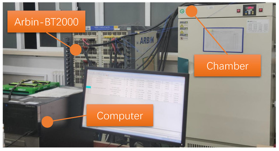
Figure 1.
The battery test platform.
Several soft pack ternary polymer LIBs of high specific energy type from Life’s Good (LG) company were used in this study. The battery has a rated capacity of 36 Ah, the negative electrode material is graphite, and the positive electrode material is typically a mixture of nickel, cobalt, and manganese, also known as NCM. Detailed information is listed in Table 1. All cells underwent a constant current–constant voltage (CC-CV) charging protocol with the current rate of 1C in the CC phase. After charging to the upper cut-off voltage of 4.15 V, the cells entered the CV phase, kept the voltage constant, and continued charging until the current dropped to 0.05C and then stopped charging. A constant current (1C) discharge was implemented until the voltage reached the lower cut-off limit of 2.5 V. Between repeat cycles of the standard charge and discharge regime, the cells also needed to rest for 2 min. During the cyclic aging test, the cells were placed in a 35 °C chamber to ensure continuous ambient temperature. The true discharge capacity can be calculated from the voltage and current measured in real-time during each cycle and, therefore, can be regarded as the temporal maximum available capacity, characterizing the battery’s health status. After each 100 charge/discharge cycle, the cells were ushered in for a performance check to recalibrate the maximum available capacity under present conditions. The chamber temperature should be set to 25 °C before the performance test experiment, and the cells must be held in it for a while so that the temperature is consistent inside and outside. The above steps are repeated until the cell reaches EOL and stops the experiment. The failure threshold is set to a 20% decay of the rated capacity, i.e., from 36 Ah to 28.8 Ah.

Table 1.
Parameters of the battery for the cycle life test.
The capacity degradation evolution trajectories can be described by the discharge capacity versus the number of cycles, as illustrated in Figure 2. Since these capacity degradation data are sequentially arranged in the order of cycle numbers, they can be considered a type of time series. It is worth remarking that since these cells are cycled under the same protocol, they follow a similar deterioration route at the early aging stage, and all exhibit a linear decrease trend. However, as the cycle continues, the capacity suddenly and sharply accelerates the decay and rapidly reaches the failure threshold, leading to an overall non-linear deterioration. Such gustily accelerated aging after a period of expected degradation can induce deviations in the lifetime profiles, probably attributed to the ongoing degradation of the kinetic properties due to the lithium precipitation from the negative electrode during the aging process, thereby weakening its performance. These discrepancies are dependent on specific cells and their degradation mechanism. It can also be observed from Figure 2 that the capacity degradation is not strictly monotonically decreasing but has local capacity regeneration phenomena, which is manifested in the fade curve as an unexpected increase at certain cycle numbers. It is because the performance tests after every 100 charge/discharge cycles will change the battery temperature and current rate, which results in significantly higher capacity readings for some cycles after testing compared to the few cycles before testing. Furthermore, in addition to the capacity regeneration-induced abrupt changes in the capacity degradation curve, there are also some unsmooth ‘spike’ points and outliers that deviate significantly from the overall trend, as shown in the enlarged subgraph. Some are due to the testing equipment itself, while others are caused by incorrect data resulting from unexpected experimental conditions, commonly called noise. These pose additional challenges for accurate lifetime prediction.
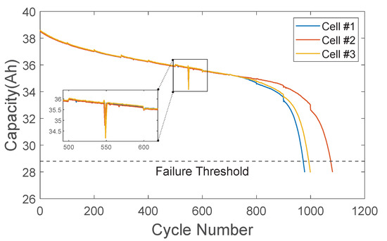
Figure 2.
The capacity degradation evolution trajectories of experimental cells ( the subplot zooms in portions of the curves with obvious outliers).
In a series-connected battery pack system, a dramatic capacity degradation of a single cell can seriously diminish the performance of the whole pack and even lead to safety problems. Therefore, it is crucial to develop a lifetime prediction model. The data obtained from the battery cyclic aging life tests can be used to evaluate the performance of the developed model in practical applications, especially for scenarios where the operating conditions are largely maintained stably.
3. Methodology
3.1. The Overall Framework
In this paper, we propose a novel LIB lifetime prediction approach entitled CGSAI for simultaneous SOH estimation and RUL prediction, with an overall framework presented in Figure 3. The expanded description is elaborated below.
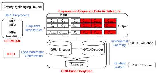
Figure 3.
The overall framework of the proposed lithium-ion battery lifetime prediction approach.
First, the capacity degradation time series are obtained through the battery cyclic aging lifetime test experiment, for which the recorded original data are preprocessed to recorrect outliers. Then, due to the noise and capacity regeneration phenomena caused by the performance test, the CEEMDAN algorithm is required to decompose the preprocessed sequence, extract the main components, and reconstruct the capacity degradation sequence. In the reconstructed battery capacity degradation time series, for a specific time step t, the w data before it constitutes an input sequence, while the k data after it comprises the corresponding output sequence. Since both inputs and outputs are sequences, this forms the Seq2Seq prediction problem. Later, a GRU-based Seq2Seq network with an attention mechanism is built to predict the battery lifetime. At the same time, an improved PSO algorithm is implemented to automatically optimize the network’s hyperparameters and achieve the optimal network structure. Finally, when evaluating SOH, the model will continuously obtain the latest online data on capacity degradation, perform incremental learning, dynamically update the parameters, and predict the capacity value for the subsequent cycles. As for the RUL prediction, the model will use the historical data for training, outputting the capacity value, and refeeding it back as input for iterating the prediction, eventually deriving the battery RUL.
3.2. Complete Ensemble Empirical Mode Decomposition with Adaptive Noise
The CEEMDAN algorithm is an enhancement of the EMD algorithm, which solves the transfer of white noise from high to low frequencies by continuously adding pairs of positive and negative Gaussian white noise during decomposition [47]. This adaptive noise processing effectively simplifies the parameter search in the traditional EMD algorithm and reduces the influence of mode mixing in the decomposition results.
As previously mentioned, the signal awaiting decomposition is the preprocessed capacity degradation time series, which can be expressed as . Then the detailed steps to decompose the signal by using the CEEMDAN algorithm are as follows.
For the , the Gaussian white noise that meets the standard normal distribution is added M times to construct the sequence waiting to be decomposed. It can be expressed by the following equation
where is the sequence with the addition of white noise, represents the signal-to-noise ratio of the original signal to the white noise, and is the white noise of i-th order.
The EMD decomposition is implemented separately on the new M sequences to obtain the first-order IMF components, and the mean of all the first-order IMF components is taken as the first-order IMF of the CEEMDAN, which satisfies the following equation
Then, the residual component is derived by subtracting the from the . It is expressed as the following equation:
Add the first-order IMF component derived by EMD decomposition of only white noise to the residual component as the new signal to be decomposed, continue to implement EMD decomposition, and repeating the steps of Equation (2) will yield the second-order IMF component, as given in the following:
where denotes the decomposition process for solving the j-th order IMF component.
For the residual components of second and subsequent orders, all can be calculated by using the formula below.
Continuing to add the j-th order component of white noise to the residual part, the -th order IMF component can be calculated by the following equation:
After repeating the steps of Equations (5) and (6) until the residual signal cannot be decomposed, all the processes of CEEMDAN are completed. The original signal is ultimately decomposed into a combination of J IMF components and residual terms, described in the following equation:
The IMFs of each order obtained from the decomposition represent the vibration modes inside the original sequence with different frequencies and amplitudes, which can characterize distinct features in the signal, respectively. In order to acquire the features that best characterize the capacity degradation trend of LIBs, correlations need to be calculated between the IMFs of each order and the original sequence. The correlation between the two sequences is generally calculated using the Pearson correlation coefficient [48], expressed by the following formula:
where X and Y are two sequences, denotes the covariance, and indicate the standard deviation, and the and represent the mean value.
Here, the IMF obtained from the CEEMDAN with the highest correlation to the original sequence after preprocessing is adopted to reconstruct the capacity degradation sequence. The specific results of decomposition and reconstruction are given in Section 4.1.
3.3. GRU-Based Seq2Seq Model with Attention Mechanism
3.3.1. Gate Recurrent Unit Neural Network
The GRU has improved the computation on hidden states of traditional RNNs by introducing the reset gate and update gate mechanism to control the information flow [49]. It makes up for the deficiency of RNN’s poor memory for long-timescale sequences and better captures the dependencies between time series data with large time step distances. The architecture of the GRU network is presented in Figure 4.
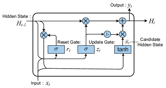
Figure 4.
The internal structure of the GRU neural network.
In the GRU, the reset gate is employed to regulate the influence of the previous moment’s hidden state on the candidate hidden state at the current moment, which is calculated as follows:
where is the weight of the reset gate, indicates the input of the reset gate, which is stitched from the current moment input and the hidden state at the previous moment in the feature dimension. refers to the sigmoid activation function, which takes values between 0 and 1.
After obtaining the reset gate output, multiply it with the previous moment hidden state and calculate it with the current moment input to obtain the candidate hidden state, as shown in the following equation:
where is the candidate hidden state weight, q means the element-by-element multiplication, and the hyperbolic tangent function is denoted as tanh, which takes values between −1 and 1.
The update gate governs the influence of the candidate hidden state containing the current moment information on the hidden state update process, and its computational expression is given as follows:
where is the weight of the update gate. The range of values for the update gate is between 0 and 1, like the reset gate.
In this case, the hidden state at the current moment is derived from the following equation:
Eventually, the output of the network is as follows:
Therefore, the GRU neural networks can effectively improve the prediction accuracy of recurrent neural networks for long-time sequences by maintaining short-term memory through the reset gate and adapting long-term dependencies through the update gate.
3.3.2. Sequence-to-Sequence Model with Attention Mechanism
The Seq2Seq model is a kind of deep learning model based on the RNN applicable for sequence prediction, which breaks the limitation that the sequence length must be fixed in traditional RNN [50]. It generally comprises three parts: encoder, decoder, and context vector, as shown in Figure 5.
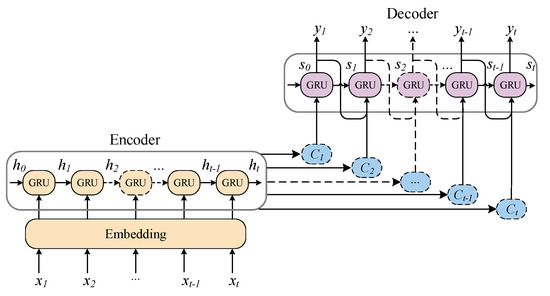
Figure 5.
The structure of Seq2Seq model with attention mechanism.
For the current moment t, the encoder maps the input sequence to the context vector that stores the semantic information in the input sequence. The following equation can derive the hidden state of the encoder output:
where denotes the encoder neural network model; here, the GRU network is used. is the input at the current moment, is the hidden state of the encoder at the previous moment, and for the initial state , it is usually set to 0.
The attention mechanism dynamically adjusts the attention weights to change the model attention level on different parts of the input sequence, enabling the decoder output at different time steps to accurately capture the corresponding parts of the input sequence and improve the model prediction accuracy. The attention weights are calculated based on the similarity between the decoder current hidden state and the i-th output hidden state of the encoder, as shown in the following equation:
where is the attention weight, which characterizes the correlation between the i-th element of the input sequence and the current output, T is the length of the input sequence, and denotes the similarity, which is calculated by the following equation:
where represents the similarity calculation function, which usually uses feedforward neural networks.
Taking a weighted average of the computed attention weights and the output of the encoder, the context vector at the current moment is derived as follows:
Finally, the decoder output at the current moment is derived as follows:
where is the output function of the decoder as well as the GRU network.
Using the GRU-based Seq2Seq model with the attention mechanism to predict battery life makes it possible to focus the prediction results more accurately on the specific part of the corresponding capacity degradation sequence, reduce the prediction error, and improve the model generalization ability.
3.4. Improved Particle Swarm Optimization Algorithm
The PSO algorithm is a global optimization algorithm based on group information intelligence, which can execute efficient exploration in the hyperparameter space and finally obtain the optimal global solution [51]. Therefore, it has been widely employed and studied in deep learning models for hyperparameter search optimization.
In the PSO algorithm, each potential optimization problem solution can be represented by a particle in the search space, where the dimension of the particle corresponds to the number of hyperparameters to be optimized, and the particle movement expresses the progress of the search process. Each particle has two attributes: position and velocity. The position is a vector composed of the current values of the hyperparameters, while the velocity determines the direction and magnitude the particle moves. The particles evaluate the quality of their current position based on the fitness function. During the movement process, the best position found by each particle itself is called the individual best, while the best position found by the entire swarm of particles is called the global best. Iterations update the speed and position of the particles, and finally, the global optimum satisfying the conditions is reached.
Suppose that N particles are initialized in the D-dimensional parameter space, and for each particle, its position vector and velocity vector are given as follows:
After setting the fitness function, the PSO updates the particle velocities by the following formula:
where is the velocity of the current particle i in the -th iteration, is the inertia weight of the particle, denotes the individual best, is the global best, and are learning factors, and and are random numbers in the interval [0, 1].
Then, the positions of the particles are updated, as given in the following equation:
where is the updated particle position.
In the early iterations of the classical PSO, the value of is relatively large, and the particles move faster, making it easier to escape local optima and exhibit a strong global search capability. As the iterations proceed, the value of gradually decreases, the particle movement becomes slower, and the global search capability weakens, making it more prone to getting trapped in local optima. Typically, and are set to the same value ranging from 0 to 2. However, this can lead to oscillations between global and local searches, reducing the search efficiency and increasing the number of iterations required.
Therefore, we propose an IPSO algorithm that makes two improvements to the traditional PSO. On the one hand, the variation of is controlled using a quadratic recession, which is calculated as follows:
where and denote the maximum and minimum values of inertia weights, respectively, k is the number of iterations, and is the total number of iterations.
On the other hand, let decrease with each iteration while the value of is increased oppositely. The improved computational formulas are as follows:
where and denote the maximum and minimum values of the learning factor, respectively.
By making dual improvements to the inertia weight and learning factor, the IPSO algorithm balances the global and local searches during the search for hyperparameters. This speeds up the search process and delivers an improvement in the accuracy of the search. The specific results of hyperparameter optimization are described in Section 4.2.
4. Result and Discussion
To verify the performance of the proposed model, SOH evaluation and RUL prediction are performed for each cell separately, and the performance is compared with the traditional RNN model and the stacked GRU model. The code runs on Python 3.8, the deep learning framework used is Tensorflow 2.6, and the hardware platform is a Win10 64-bit workstation with an Intel(R) Xeon(R) Gold 5218 CPU @2.30GHz and an NVIDIA GeForce RTX 3090 24GB graphics card.
4.1. The Reconstruction of Capacity Degradation Sequences
The results of each order IMF components and residuals obtained by CEEMDAN for the preprocessed battery capacity degradation time series are displayed in Figure 6. The most correlated IMF components (IMF5 for all three cells) are marked with red lines for observation. It can be clearly observed that when the CEEMDAN algorithm is implemented, the intermittent signal components (IMF1 and IMF2) containing high frequencies with approximately zero-averaged amplitudes are obtained first. Then the sequence’s low and medium-frequency components (IMF3 and IMF4) are extracted. Finally, the component with the largest amplitude (IMF5) and the residue term with many non-periodic perturbations of tiny amplitude is attained. Among them, IMF5 shows the most significant magnitude and smooth curve similar to the original capacity degradation sequence, indicating that it characterizes the most critical degradation trend in the capacity degradation sequence of LIB and plays an essential role in explaining capacity degradation. The small amplitude of the residual term (less than in absolute value) further indicates that the sequence is well decomposed, and most of the signals can be described by the IMF component.
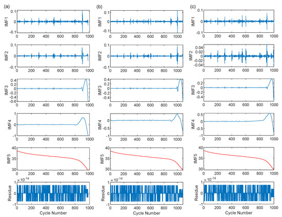
Figure 6.
The results of battery capacity degradation sequence by the CEEMDAN decomposition. (a) The result of cell #1. (b) The result of cell #2. (c) The result of cell #3.
Table 2 gives the Pearson correlation coefficients between the preprocessed capacity degradation time series and the IMF components of each order. From Table 2, it can be noticed that the initial IMFs obtained during the decomposition are not strongly correlated with the battery capacity degradation. As the decomposition proceeds, the subsequent IMFs become increasingly related to capacity degradation, and the IMF with the highest correlation is gained at the end of the decomposition process. By reconstructing the capacity degradation time series using the IMF component with the highest correlation, the primary trend of the degradation can be captured to the greatest extent while minimizing the impact of noise. The reconstructed sequences are then used as the training data for the deep learning model to predict future capacity degradation. This approach can help the model avoid learning irrelevant features and improve its generalization ability.
Table 2.
The Pearson correlation coefficients between preprocessed capacity degradation series and IMFs.
4.2. Hyperparameter Optimization
When building the deep learning model for battery lifetime prediction, the model hyperparameters must first be determined, such as the number of layers, the number of neurons per layer, and the learning rate. Generally speaking, more layers will confer stronger learning ability to the model in deep learning. However, overly deep networks also increase the model complexity and tend to cause overfitting. Since the cycle life of all batteries does not exceed 1500 cycles, and the sample size of the capacity degradation is not very large, it is inappropriate to set an excessively deep network. Here, the number of layers for the encoder is set to 2, and for the decoder is set to 1 layer. The length of the input sequence is set to 10, and the size of the output sequence is set to 5. The remaining hyperparameters that need to be optimized are the number of neurons in each layer of the encoder, the number of neurons in the decoder, and the learning rate of the entire network. Therefore, the search space for hyperparameters is six dimensions. Then, each hyperparameter is constrained within a certain range: the number of neurons in each layer ranges from 8 to 4096, with an increasing step size of 8. The learning rate varies from to , with an increasing step size of 5 times, and any learning rate exceeding the upper limit is directly set to the upper limit value.
The model uses the mean square error (MSE) as the loss function and the stochastic gradient descent (SGD) as the optimizer to update the gradient and guide the convergence of parameters. The fitness function of the IPSO algorithm optimizes the hyperparameters by tracking the loss of the model. Initializing the positions and velocities of 50 particles and executing 200 iterations, the loss variation trend of the IPSO algorithm during the search of each cell model is demonstrated in Figure 7 compared with the traditional PSO algorithm.
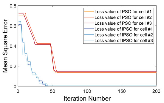
Figure 7.
The variation trend of loss for the IPSO algorithm and traditional PSO algorithm.
Figure 7 demonstrates that as the number of iterations increases, both the PSO and IPSO exhibit a decreasing trend in loss, indicating that the algorithms are searching along the appropriate direction of hyperparameters. However, the traditional PSO algorithm falls into a locally optimal solution at about 50 iterations and cannot further reduce the loss. In contrast, the IPSO algorithm performs comparably to the PSO algorithm after about 25 iterations. And it can jump out of the local optimum as the iterations proceed, achieving better convergence. Compared with the traditional PSO algorithm, the IPSO algorithm performs better regarding iteration speed and final results.
The optimal combination of hyperparameters discovered by the IPSO algorithm is given in Table 3. As can be seen, the number of neurons required to establish the model varies due to the different lengths of the capacity degradation time series. Specifically, batteries with shorter cycle life require fewer neurons overall, and the number of neurons in the first encoder layer is more than that in the second layer, which is to extract the features of the input sequence better. Meanwhile, the number of neurons in the decoder layer differs slightly from that in the second layer, which can better decode the features and generate the output sequence. The optimal combination of hyperparameters determined by using the IPSO algorithm is used to build the model and trained to achieve the prediction of battery lifetime ultimately.
Table 3.
The optimal combination of hyperparameters.
4.3. Online SOH Evaluation
The online SOH evaluation is enabled by incremental learning of the online data. For each cell, the existing capacity degradation data is treated as historical data and utilized to train the initial model. As the battery is cycled, new online capacity data is accessed and fed into the initial model. Then, the parameters are updated to improve the model accuracy to fit the latest data.
The amount of historical data utilized for training influences the initial model accuracy, which in turn determines the subsequent incremental learning outcomes. Training a model for online SOH evaluation with various quantities of historical data can also be referred to predict from different start points (SPs). In this section, online SOH evaluation is conducted in the early (SP = 20%), middle (SP = 50%), and late (SP = 80%) periods of battery operation, and accordingly, data before SP are used to train the model. The stacked conventional GRU and RNN models without the Seq2Seq structure are compared to validate the improvement of the proposed method on model accuracy through incremental learning. The number of network layers and other hyperparameters used for comparison are the same as those of the Seq2Seq model.
The results of the online SOH evaluation for the three cells are illustrated in Figure 8. As can be observed from the figure, for all cells, the conventional GRU and RNN models fail to learn the relatively accurate battery decline trend when only the first 20% of the data are used to train the initial model. Therefore, even if the capacity data is continuously updated for incremental learning, the two models need help reducing errors and showing significant differences in the subsequent SOH evaluation. In the linear battery decline stage, the SOH evaluation result of the RNN model is almost the same as the true value, which is more reliable. In contrast, although the GRU model can also portray this linear decline, the prediction deviates far from the actual value. When entering the late decline stage, the battery shows an apparent nonlinear degradation. The RNN model cannot capture the change of this declining trend, while the GRU model can track this accelerated aging behavior but is unable to reduce the prediction error. Evidently, the Seq2Seq model proposed in this paper benefits from applying the attention mechanism, accurately predicting both capacity recovery during linear degradation and accelerated aging during nonlinear degradation. The resulting curves are almost identical to the actual SOH changes. Moreover, as the amount of training data used to establish the initial model increases, the model accuracy also improves. Overall, the SOH evaluation results obtained using the Seq2Seq model are the closest to the actual situation, followed by the GRU model. The performance of the RNN model is limited by its own architecture, and even when using 80% of the data for training, it is still unable to predict the nonlinear degradation of the battery accurately.
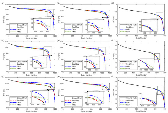
Figure 8.
The results of online SOH evaluation from different SPs for the cells. (a) Cell #1 SP = 20%. (b) Cell #1 SP = 50%. (c) Cell #1 SP = 80%. (d) Cell #2 SP = 20%. (e) Cell #2 SP = 50%. (f) Cell #2 SP = 80%. (g) Cell #3 SP = 20%. (h) Cell #3 SP = 50%. (i) Cell #3 SP = 80%.
The numerical values of the mean absolute error (MAE), root mean square error (RMSE), and mean absolute percentage error (MAPE) of the SOH evaluation results for each model at different SPs of these cells are listed in Table 4. The smaller the metrics values in the table, the better the predictive performance of the model. It is clear from the table that for all cells, whether in the early (SP = 20%), middle (SP = 50%), or late stage (SP = 80%) of use, the proposed Seq2Seq model performs the best in the SOH evaluation. Moreover, as the amount of training data increases, the predictive performance of all three models improves. In other words, more training data lead to more accurate predictive models. Among them, the prediction performance of the Seq2Seq model, when using only the first 20% of data for training, is even better than that of the traditional GRU and RNN models trained with 80% of the data. Specifically, when evaluating the SOH at 20% of the cycle life, the Seq2Seq model outperforms the traditional GRU and RNN models in terms of all three metrics compared to monitoring at 80% of the battery lifetime.
Table 4.
The assessment metrics of the SOH evaluation results for each model.
Meanwhile, for the three cells, the GRU model has worse results than the RNN model for SOH evaluation at 20% of the cycle life, except for the RMSE metric on cell #2, where the GRU model’s 0.5390 is slightly smaller than the RNN model’s 0.7440. However, when the training data increase to 50%, the three metrics of the GRU model and the RNN model become superior and inferior to each other. And when the amount of training data reach 80%, all metrics of the GRU model are smaller than those of the RNN model. The changing trend of the GRU and the RNN model in predicting metrics is consistent with the SOH evaluation results shown in the previous figures. Although the GRU model can track the accelerated degradation of the battery, it predicts the linear degradation of the battery poorly in the early and middle stages of use. On the other hand, although the RNN model can accurately predict the linear degradation of the battery, it cannot capture the nonlinear accelerated aging of the battery in the later stages of use.
The results above provide additional evidence of the superiority of the Seq2Seq model proposed in this paper. Furthermore, this accurate prediction of future multi-step SOH evaluation implies a small error when using the model to predict all subsequent capacity decays. This provides a reasonable basis for long-horizon iterative RUL prediction.
4.4. Iterative RUL Prediction
The iterative RUL prediction is performed by using the reconstructed capacity data of the remaining two cells and the first 30% and 50% of the recession data of the test battery as training, and the model parameters are not changed once the model is trained. The model is then employed to predict the subsequent capacity, and the predicted capacity is considered input data to continue the iterative prediction until the model output capacity is below the battery failure threshold to obtain the RUL prediction results.
Similarly to the online SOH evaluation, the iterative RUL prediction for each cell at 30% SP and 50% SP for the Seq2Seq model and the conventional GRU and RNN models are illustrated in Figure 9. The abscissa is the cycle number, the ordinate is the cell capacity, and the black horizontal dashed line is the capacity failure threshold of the cell, which here is 28.8Ah. By finding the intersection of the prediction curve and the failure threshold, the corresponding value on the horizontal axis is identified as the end-of-prediction (EOP) of the battery cycle life. The difference between the EOP and the SP cycle number is the predicted RUL of the battery.
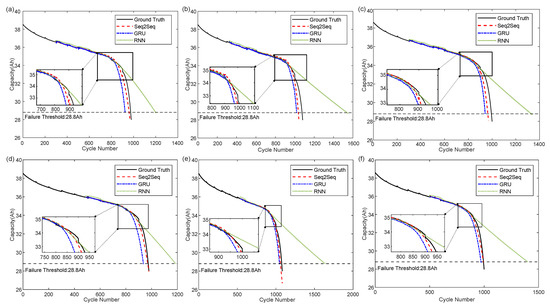
Figure 9.
The results of iterative RUL prediction. (a) At 30% SP for cell #1. (b) At 30% SP for cell #2. (c) At 30% SP for cell #3. (d) At 50% SP for cell #1. (e) At 50% SP for cell #2. (f) At 50% SP for cell #3.
As can be noted from the figure, the Seq2Seq model has a more complete and accurate learning of the battery capacity degradation trend due to the use of the entire capacity degradation time series data of the remaining two cells for training. It performs better than other methods when dealing with long-cycle time series, and the prediction curves are closer to the real curves. As shown in Figure 9a–c, when we train the model using the degradation data of the remaining two cells and the first 30% of the test cell, the EOP values obtained by the Seq2Seq model on the three cell data sets are 959, 1037, and 964 cycles, respectively. Compared with the corresponding real EOL values of 974, 1076, and 995 cycles, the differences are 11, 39, and 31 cycles. It indicates that fine-tuning the model using only the first 30% of the degradation data can obtain a relatively good trajectory of the capacity degradation on the iterative RUL predictions. However, the EOP predictions still have errors of more than 10 cycles.
When the data are increased to the first 50% SP, the EOP values obtained by the Seq2Seq model on the three cell data sets are 970, 1059, and 994 cycles, respectively, as displayed in Figure 9d–f. The differences are only 4, 17, and 1 cycles compared to the corresponding actual EOL values. Although the conventional GRU model has relatively effective prediction results in the linear degradation stage of the battery, it is affected by cumulative errors during the iterative prediction process. Therefore, compared with the prediction results of the Seq2Seq model, the GRU model enters the non-linear degradation process earlier, with predicted EOP values of 937, 1047, and 972 cycles, separately. The conventional RNN model shows significant errors at the beginning of prediction, which are gradually corrected during iterative prediction in the linear degradation stage. The predicted curve becomes closer to the actual value. However, with further iteration, the RNN model accumulates more prediction errors. As the battery enters the nonlinear accelerated aging, the model is unable to predict this degradation trend and still maintains the linear degradation, leading to the most significant deviation from the actual value, with predicted EOP values of 1187, 1637, and 1401 cycles, correspondingly.
To further expound the superiority of the proposed Seq2Seq model in predicting long-timescale LIB capacity degradation sequences, Table 5 presents detailed RUL actual values, predicted values, absolute errors (AE), relative errors (RE), as well as the MAE, RMSE, MAPE, and decision coefficient () of the predicted sequences for the three cells at 50% SP.
Table 5.
The assessment metrics of the RUL prediction results for each model at 50% SP.
From the table, it can be seen that the AEs between the RUL predicted by the Seq2Seq model and the true values are −4, −17, and −1, and the REs are −0.8214%, −3.1598%, and −0.2008%, which are numerically much lower than the prediction errors of the other two models. In terms of the evaluation metrics of the predicted sequence and the true capacity degradation sequence, the Seq2Seq model also outperforms the other two models to a large extent, and the evaluation metrics of the GRU model are generally better than those of the RNN model. However, on the cell #1 data, the MAE, RMSE, MAPE, and of the GRU model are 0.1985, 0.5895, 0.5881, and 0.9325, respectively, which are slightly inferior to 0.1946, 0.4033, 0.5768, and 0.9532 of the RNN model. This is because when calculating the evaluation metrics between sequences, it is necessary to maintain consistency in sequence length. For the Seq2Seq model and the GRU model, since the predicted sequence length is shorter than the true sequence length, the calculation is based on the shorter sequence. In contrast, the RNN model predicts a much longer sequence than the true sequences and needs to adopt the true sequences as the calculated benchmark. In the case of cell #1 data, the predicted sequence length of the GRU model is 937, and the true sequence length is 974, so only the evaluation metrics between 937 pairs of data points are calculated. The predicted sequence length of the RNN model is 1187, and the evaluation metrics between 974 data points need to be calculated. Moreover, the RNN model has lower prediction errors in the linear degradation stage of cell #1 compared to the GRU model. Hence, the evaluation metrics of the RNN model on cell #1 data are slightly better than those of the GRU model. The values of the decision coefficient for the three models are higher than 0.9, indicating that the predicted curve is very close to the true curve. The of the Seq2Seq model is as high as 0.99, further demonstrating the superiority over the other two models.
In summary, the proposed Seq2Seq model has a stronger learning ability for long-timescale LIB capacity degradation sequences, and the iterative RUL prediction results are more stable and accurate.
5. Conclusions
SOH evaluation and RUL prediction are crucial for the battery management system. In this paper, we propose a new lifetime prediction framework for LIB called CGSAI, which can simultaneously achieve the above two functions. This new method first uses the CEEMDAN method to decompose the battery capacity degradation sequence, which solves the problems of mode mixing, endpoint effects, and sieving iteration-stopping criteria brought about by the traditional EMD. Meanwhile, the IMF component with the highest correlation is selected to reconstruct the degradation sequence as the training data, effectively avoiding the influence of noise in the original data on prediction accuracy. Then the GRU-based Seq2Seq model is established, and the attention mechanism is introduced to dynamically assign attention weights to each time step during the calculation process based on the current decoder state and encoder output, improving network prediction performance. Next, we improve the traditional PSO algorithm from both the inertial weight and learning factor aspects and use the improved IPSO algorithm for automatic hyperparameter search of the Seq2Seq model to speed up convergence and avoid local optima, thereby improving the efficiency and accuracy of optimization. Finally, SOH evaluation and RUL prediction are realized using online capacity measurements and updated historical data, respectively. On the battery data set under fixed working conditions, the proposed method outperformed traditional GRU and RNN models. The predicted MAPE on the online SOH evaluation can reach a minimum of 0.76%, the absolute error on the iterative prediction of RUL is not more than 17 cycles, and the MAPE is not more than 0.27%.
Author Contributions
Conceptualization, D.C. and W.Z.; Data curation, Formal analysis, Methodology, Software, and Writing—original draft, D.C.; Project administration and Supervision, W.Z.; Funding acquisition, C.Z. and B.S.; Writing—review & editing, C.Z., B.S., H.C., S.Y. and X.C. All authors have read and agreed to the published version of the manuscript.
Funding
This research was funded by the National Key Research and Development Program of China (Grant No. 2022YFB2502304), the Joint Fund of Ministry of Education of China for Equipment Pre-research (Grant No. 8091B022130), the Young Scientists Fund of the National Natural Science Foundation of China (Grant No. 52222708), and the National Natural Science Foundation of China (Grant No. 52177206 and 51977007).
Conflicts of Interest
The authors declare no conflict of interest.
References
- Jiang, Y.; Jiang, J.; Zhang, C.; Zhang, W.; Gao, Y.; Mi, C. A Copula-based battery pack consistency modeling method and its application on the energy utilization efficiency estimation. Energy 2019, 189, 116219. [Google Scholar] [CrossRef]
- Ouyang, M.; Feng, X.; Han, X.; Lu, L.; Li, Z.; He, X. A dynamic capacity degradation model and its applications considering varying load for a large format Li-ion battery. Appl. Energy 2016, 165, 48–59. [Google Scholar] [CrossRef]
- Schmuch, R.; Wagner, R.; Hörpel, G.; Placke, T.; Winter, M. Performance and cost of materials for lithium-based rechargeable automotive batteries. Nat. Energy 2018, 3, 267–278. [Google Scholar] [CrossRef]
- Xiong, R.; Zhang, Y.; He, H.; Zhou, X.; Pecht, M.G. A Double-Scale, Particle-Filtering, Energy State Prediction Algorithm for Lithium-Ion Batteries. IEEE Trans. Ind. Electron. 2018, 65, 1526–1538. [Google Scholar] [CrossRef]
- Han, X.; Lu, L.; Zheng, Y.; Feng, X.; Li, Z.; Li, J.; Ouyang, M. A review on the key issues of the lithium ion battery degradation among the whole life cycle. eTransportation 2019, 1, 100005. [Google Scholar] [CrossRef]
- Liu, Y.H.; Luo, Y.F. Search for an Optimal Rapid-Charging Pattern for Li-Ion Batteries Using the Taguchi Approach. IEEE Trans. Ind. Electron. 2010, 57, 3963–3971. [Google Scholar] [CrossRef]
- Severson, K.A.; Attia, P.M.; Jin, N.; Perkins, N.; Jiang, B.; Yang, Z.; Chen, M.H.; Aykol, M.; Herring, P.K.; Fraggedakis, D.; et al. Data-driven prediction of battery cycle life before capacity degradation. Nat. Energy 2019, 4, 383–391. [Google Scholar] [CrossRef]
- Meng, J.; Cai, L.; Stroe, D.I.; Ma, J.; Luo, G.; Teodorescu, R. An optimized ensemble learning framework for lithium-ion Battery State of Health estimation in energy storage system. Energy 2020, 206, 118140. [Google Scholar] [CrossRef]
- Zhang, Y.; Peng, Z.; Guan, Y.; Wu, L. Prognostics of battery cycle life in the early-cycle stage based on hybrid model. Energy 2021, 221, 119901. [Google Scholar] [CrossRef]
- Wang, Q.; Wang, Z.; Zhang, L.; Liu, P.; Zhou, L. A Battery Capacity Estimation Framework Combining Hybrid Deep Neural Network and Regional Capacity Calculation Based on Real-World Operating Data. IEEE Trans. Ind. Electron. 2023, 70, 8499–8508. [Google Scholar] [CrossRef]
- Zhang, L.; Hu, X.; Wang, Z.; Sun, F.; Deng, J.; Dorrell, D.G. Multiobjective Optimal Sizing of Hybrid Energy Storage System for Electric Vehicles. IEEE Trans. Veh. Technol. 2018, 67, 1027–1035. [Google Scholar] [CrossRef]
- Wang, C.; Chen, Y.; Zhang, Q.; Zhu, J. Dynamic early recognition of abnormal lithium-ion batteries before capacity drops using self-adaptive quantum clustering. Appl. Energy 2023, 336, 120841. [Google Scholar] [CrossRef]
- Li, X.; Wang, Z.; Zhang, L.; Zou, C.; Dorrell, D.D. State-of-health estimation for Li-ion batteries by combing the incremental capacity analysis method with grey relational analysis. J. Power Sources 2019, 410–411, 106–114. [Google Scholar] [CrossRef]
- Voronov, S.; Frisk, E.; Krysander, M. Data-Driven Battery Lifetime Prediction and Confidence Estimation for Heavy-Duty Trucks. IEEE Trans. Reliab. 2018, 67, 623–639. [Google Scholar] [CrossRef]
- Wang, D.; Zhao, Y.; Yang, F.; Tsui, K.L. Nonlinear-drifted Brownian motion with multiple hidden states for remaining useful life prediction of rechargeable batteries. Mech. Syst. Signal Process. 2017, 93, 531–544. [Google Scholar] [CrossRef]
- Li, X.; Yu, D.; Søren Byg, V.; Daniel Ioan, S. The development of machine learning-based remaining useful life prediction for lithium-ion batteries. J. Energy Chem. 2023, 82, 103–121. [Google Scholar] [CrossRef]
- Jiang, J.; Ruan, H.; Sun, B.; Wang, L.; Gao, W.; Zhang, W. A low-temperature internal heating strategy without lifetime reduction for large-size automotive lithium-ion battery pack. Appl. Energy 2018, 230, 257–266. [Google Scholar] [CrossRef]
- Hu, X.; Li, S.; Peng, H. A comparative study of equivalent circuit models for Li-ion batteries. J. Power Sources 2012, 198, 359–367. [Google Scholar] [CrossRef]
- Kemper, P.; Li, S.E.; Kum, D. Simplification of pseudo two dimensional battery model using dynamic profile of lithium concentration. J. Power Sources 2015, 286, 510–525. [Google Scholar] [CrossRef]
- Tian, J.; Xu, R.; Wang, Y.; Chen, Z. Capacity attenuation mechanism modeling and health assessment of lithium-ion batteries. Energy 2021, 221, 119682. [Google Scholar] [CrossRef]
- Yang, F.; Song, X.; Dong, G.; Tsui, K.L. A coulombic efficiency-based model for prognostics and health estimation of lithium-ion batteries. Energy 2019, 171, 1173–1182. [Google Scholar] [CrossRef]
- Ouyang, T.; Xu, P.; Lu, J.; Hu, X.; Liu, B.; Chen, N. Coestimation of State-of-Charge and State-of-Health for Power Batteries Based on Multithread Dynamic Optimization Method. IEEE Trans. Ind. Electron. 2022, 69, 1157–1166. [Google Scholar] [CrossRef]
- Lai, X.; Huang, Y.; Han, X.; Gu, H.; Zheng, Y. A novel method for state of energy estimation of lithium-ion batteries using particle filter and extended Kalman filter. J. Energy Storage 2021, 43, 103269. [Google Scholar] [CrossRef]
- Walker, E.; Rayman, S.; White, R.E. Comparison of a particle filter and other state estimation methods for prognostics of lithium-ion batteries. J. Power Sources 2015, 287, 1–12. [Google Scholar] [CrossRef]
- Wang, S.; Fernandez, C.; Yu, C.; Fan, Y.; Cao, W.; Stroe, D.I. A novel charged state prediction method of the lithium ion battery packs based on the composite equivalent modeling and improved splice Kalman filtering algorithm. J. Power Sources 2020, 471, 228450. [Google Scholar] [CrossRef]
- Xu, X.; Chen, N. A state-space-based prognostics model for lithium-ion battery degradation. Reliab. Eng. Syst. Saf. 2017, 159, 47–57. [Google Scholar] [CrossRef]
- Chang, Y.; Fang, H.; Zhang, Y. A new hybrid method for the prediction of the remaining useful life of a lithium-ion battery. Appl. Energy 2017, 206, 1564–1578. [Google Scholar] [CrossRef]
- Remaining useful life prediction of lithium-ion battery with unscented particle filter technique. Microelectron. Reliab. 2013, 53, 805–810. [CrossRef]
- Cong, X.; Zhang, C.; Jiang, J.; Zhang, W.; Jiang, Y.; Jia, X. An Improved Unscented Particle Filter Method for Remaining Useful Life Prognostic of Lithium-ion Batteries with Li(NiMnCo)O2 Cathode with Capacity Diving. IEEE Access 2020, 8, 58717–58729. [Google Scholar] [CrossRef]
- Fei, Z.; Yang, F.; Tsui, K.L.; Li, L.; Zhang, Z. Early prediction of battery lifetime via a machine learning based framework. Energy 2021, 225, 120205. [Google Scholar] [CrossRef]
- Ma, G.; Zhang, Y.; Cheng, C.; Zhou, B.; Hu, P.; Yuan, Y. Remaining useful life prediction of lithium-ion batteries based on false nearest neighbors and a hybrid neural network. Appl. Energy 2019, 253, 113626. [Google Scholar] [CrossRef]
- Shu, X.; Li, G.; Shen, J.; Lei, Z.; Chen, Z.; Liu, Y. A uniform estimation framework for state of health of lithium-ion batteries considering feature extraction and parameters optimization. Energy 2020, 204, 117957. [Google Scholar] [CrossRef]
- Khelif, R.; Chebel-Morello, B.; Malinowski, S.; Laajili, E.; Fnaiech, F.; Zerhouni, N. Direct Remaining Useful Life Estimation Based on Support Vector Regression. IEEE Trans. Ind. Electron. 2017, 64, 2276–2285. [Google Scholar] [CrossRef]
- Chen, Z.; Shi, N.; Ji, Y.; Niu, M.; Wang, Y. Lithium-ion batteries remaining useful life prediction based on BLS-RVM. Energy 2021, 234, 121269. [Google Scholar] [CrossRef]
- Li, W.; Fan, Y.; Ringbeck, F.; Jöst, D.; Sauer, D.U. Unlocking electrochemical model-based online power prediction for lithium-ion batteries via Gaussian process regression. Appl. Energy 2022, 306, 118114. [Google Scholar] [CrossRef]
- Niu, G.; Wang, X.; Liu, E.; Zhang, B. Lebesgue Sampling Based Deep Belief Network for Lithium-Ion Battery Diagnosis and Prognosis. IEEE Trans. Ind. Electron. 2022, 69, 8481–8490. [Google Scholar] [CrossRef]
- Wu, J.; Zhang, C.; Chen, Z. An online method for lithium-ion battery remaining useful life estimation using importance sampling and neural networks. Appl. Energy 2016, 173, 134–140. [Google Scholar] [CrossRef]
- Zhang, Y.; Xiong, R.; He, H.; Pecht, M.G. Long Short-Term Memory Recurrent Neural Network for Remaining Useful Life Prediction of Lithium-Ion Batteries. IEEE Trans. Veh. Technol. 2018, 67, 5695–5705. [Google Scholar] [CrossRef]
- Chen, D.; Zhang, W.; Zhang, C.; Sun, B.; Cong, X.; Wei, S.; Jiang, J. A novel deep learning-based life prediction method for lithium-ion batteries with strong generalization capability under multiple cycle profiles. Appl. Energy 2022, 327, 120114. [Google Scholar] [CrossRef]
- Wang, D.; Kong, J.Z.; Zhao, Y.; Tsui, K.L. Piecewise model based intelligent prognostics for state of health prediction of rechargeable batteries with capacity regeneration phenomena. Measurement 2019, 147, 106836. [Google Scholar] [CrossRef]
- Li, X.; Zhang, L.; Wang, Z.; Dong, P. Remaining useful life prediction for lithium-ion batteries based on a hybrid model combining the long short-term memory and Elman neural networks. J. Energy Storage 2019, 21, 510–518. [Google Scholar] [CrossRef]
- Song, Y.; Li, L.; Peng, Y.; Liu, D. Lithium-Ion Battery Remaining Useful Life Prediction Based on GRU-RNN. In Proceedings of the 2018 12th International Conference on Reliability, Maintainability, and Safety (ICRMS), Shanghai, China, 17–19 October 2018; pp. 317–322. [Google Scholar] [CrossRef]
- Qian, C.; Xu, B.; Xia, Q.; Ren, Y.; Sun, B.; Wang, Z. SOH prediction for Lithium-Ion batteries by using historical state and future load information with an AM-seq2seq model. Appl. Energy 2023, 336, 120793. [Google Scholar] [CrossRef]
- Xue, B.; Zhang, M.; Browne, W.N.; Yao, X. A Survey on Evolutionary Computation Approaches to Feature Selection. IEEE Trans. Evol. Comput. 2016, 20, 606–626. [Google Scholar] [CrossRef]
- Karaboga, D.; Akay, B. A comparative study of Artificial Bee Colony algorithm. Appl. Math. Comput. 2009, 214, 108–132. [Google Scholar] [CrossRef]
- Jia, X.; Zhang, C.; Wang, L.Y.; Zhang, L.; Zhou, X. Early Diagnosis of Accelerated Aging for Lithium-Ion Batteries with an Integrated Framework of Aging Mechanisms and Data-Driven Methods. IEEE Trans. Transp. Electrif. 2022, 8, 4722–4742. [Google Scholar] [CrossRef]
- Colominas, M.A.; Schlotthauer, G.; Torres, M.E. Improved complete ensemble EMD: A suitable tool for biomedical signal processing. Biomed. Signal Process. Control 2014, 14, 19–29. [Google Scholar] [CrossRef]
- Jebli, I.; Belouadha, F.Z.; Kabbaj, M.I.; Tilioua, A. Prediction of solar energy guided by pearson correlation using machine learning. Energy 2021, 224, 120109. [Google Scholar] [CrossRef]
- Cho, K.; van Merriënboer, B.; Gulcehre, C.; Bahdanau, D.; Bougares, F.; Schwenk, H.; Bengio, Y. Learning Phrase Representations using RNN Encoder–Decoder for Statistical Machine Translation. In Proceedings of the 2014 Conference on Empirical Methods in Natural Language Processing (EMNLP), Doha, Qatar, 25–29 October 2014; pp. 1724–1734. [Google Scholar] [CrossRef]
- Sutskever, I.; Vinyals, O.; Le, Q.V. Sequence to Sequence Learning with Neural Networks. In Proceedings of the Advances in Neural Information Processing Systems; Curran Associates, Inc.: Red Hook, NY, USA, 2014; Volume 27. [Google Scholar] [CrossRef]
- Zeng, N.; Wang, Z.; Liu, W.; Zhang, H.; Hone, K.; Liu, X. A Dynamic Neighborhood-Based Switching Particle Swarm Optimization Algorithm. IEEE Trans. Cybern. 2022, 52, 9290–9301. [Google Scholar] [CrossRef]
Disclaimer/Publisher’s Note: The statements, opinions and data contained in all publications are solely those of the individual author(s) and contributor(s) and not of MDPI and/or the editor(s). MDPI and/or the editor(s) disclaim responsibility for any injury to people or property resulting from any ideas, methods, instructions or products referred to in the content. |
© 2023 by the authors. Licensee MDPI, Basel, Switzerland. This article is an open access article distributed under the terms and conditions of the Creative Commons Attribution (CC BY) license (https://creativecommons.org/licenses/by/4.0/).