Abstract
Battery degradation is a complex nonlinear problem, and it is crucial to accurately predict the cycle life of lithium-ion batteries to optimize the usage of battery systems. However, diverse chemistries, designs, and degradation mechanisms, as well as dynamic cycle conditions, have remained significant challenges. We created 53 features from discharge voltage curves, 18 of which were newly developed. The maximum relevance minimum redundancy (MRMR) algorithm was used for feature selection. Robust linear regression (RLR) and Gaussian process regression (GPR) algorithms were deployed on three different datasets to estimate battery cycle life. The RLR and GPR algorithms achieved high performance, with a root-mean-square error of 6.90% and 6.33% in the worst case, respectively. This work highlights the potential of combining feature engineering and machine learning modeling based only on discharge voltage curves to estimate battery degradation and could be applied to onboard applications that require efficient estimation of battery cycle life in real time.
1. Introduction
Lithium-ion batteries have been widely used in various applications, such as electric vehicles, battery energy storage systems (BESSs), and portable electronics, due to their high energy density, low cost, and low self-discharge rate [1]. However, similar to most complex mechanical, electrical, and chemical systems, the aging of lithium-ion batteries is inevitable due to side reactions occurring within their electrolyte and electrodes [2]. This aging process causes a decline in battery performance. Thus, it is essential to accurately predict the aging of lithium-ion batteries to ensure long-term stability and reliable operation.
Many approaches have been suggested to accurately predict the lifetime of lithium-ion batteries, including empirical models [3], equivalent circuit models [4,5,6], physical models [7], and data-driven models [2,8,9,10,11,12]. Empirical models assume that cells of the same chemistry age in the same manner [3], which may not always be the case. Equivalent circuit models are semiempirical and unable to represent various aging patterns [4], and the parameters are difficult to identify when considering different usage conditions, ambient temperatures, and load profiles [13,14,15]. Physical models consist of complex partial differential equations and require many parameters that are not easily obtainable [16,17,18]. While some studies have provided model parameters that accurately explain observed data, the accuracy of predictions may rapidly decline in the presence of uncertain mechanisms and aging rates under future usage conditions [8,18].
In contrast, data-driven models have many advantages, such as the ability to capture battery degradation mechanisms without complex chemical reaction knowledge. Recently, many studies [10,16,19,20] have used machine learning or deep learning tools for battery life estimation. Feature extraction and selection are essential for machine learning approaches. Various studies have extracted features using charge voltage curves, raw data from battery cycle tests (i.e., voltage, current, temperature, and state of charge (SOC) data) [17,21,22], discharge voltage curves [23], and electrochemical impedance spectroscopy (EIS) [12,24]. Charge and discharge voltage curves can be obtained via the battery management system (BMS) in real time [23,25], while EIS data can only be measured with an electrochemical impedance analyzer. Extracting features based on the charge voltage curve is feasible because most charge protocols are typically constant current (CC) and constant voltage (CV) [10,11,21,23]. It is challenging to derive features through the discharge voltage curve because load behaviors vary among batteries. Feature selection typically relies on background knowledge or Pearson correlation analysis, with the aim of reducing the size of the input matrix and avoiding overfitting [10,21,26,27]. However, these approaches overlook the redundancy among features.
To achieve an accurate prediction of battery life, different fitting functions with optimizable parameters have been implemented. One such method is support vector regression (SVR) [28,29,30], which has been observed to have high accuracy; however, SVR is time-consuming for model training. In contrast, linear regression (LR) with an elastic net requires a much quicker training time [31,32], but its accuracy tends to decline for large datasets. Neural network (NN) models have also been used, with the performance improving as the number of hidden layers and neurons increases [33,34]; however, neural network models are hard to train, and it is difficult to choose a network structure. Gaussian process regression (GPR) has demonstrated promising accuracy and faster training speed than SVR [10,23,35,36]; however, its complexity remains problematic, hindering onboard deployment.
This paper proposed an innovative data-driven framework for accurately and promptly predicting battery cycle lives (as in Figure 1). Using pattern recognition and signal processing techniques, battery degradation features were extracted from discharge voltage curves. Next, using the maximum relevance minimum redundancy (MRMR) algorithm, 20 of 53 features were selected as the feature subset. Three different battery datasets were used to train and test the GPR and robust linear regression (RLR) algorithms. The test results suggested that GPR outperforms RLR in most cases, while RLR has a faster prediction speed than GPR. These results illustrate the power of combining feature extraction and selection with data-driven modeling based on discharge voltage curves to predict the degradation of lithium-ion batteries.
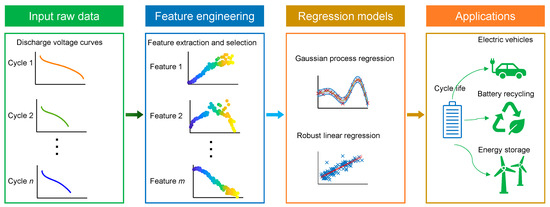
Figure 1.
Schematic diagram of battery cycle life prediction based on discharge voltage curves. The colors of the discharge voltage curves indicate that they belong to different cycles, and the colors of the curves in the feature extraction and selection box suggest that their values change as the cycle number increases.
The main contributions of this article are listed as follows:
- New features were developed using pattern recognition and signal processing techniques to capture degradation mechanisms using discharge voltage profiles.
- The MRMR algorithm was proposed for feature selection, reducing the parameter size of the model and improving the prediction speed.
- Two algorithms, GPR and RLR, were trained for battery cycle life prediction. GPR was found to have high accuracy but is time-consuming, making it best suited for battery pack manufacturing and battery recycling. Conversely, RLR requires less training time, and its accuracy is suitable for real-time battery management applications, making it ideal for onboard deployment.
The remainder of this article is organized as follows: Section 2 introduces the details of three lithium-ion battery datasets, Section 3 describes the machine learning framework, the results of feature extraction and battery cycle life prediction are presented in Section 4, and Section 5 discusses the test results. This article is concluded in Section 6.
2. Design of Battery Datasets
We deployed our methods on three different battery datasets due to the varying degradation mechanisms of lithium-ion batteries. Dataset I [33] incorporates 39 cells, cells 1 to 30 were used as the training set, and cells 31 to 39 served as the test set. The positive electrode material of the cells is a blend of lithium cobalt oxide (LCO) and ternary nickel cobalt lithium manganese (NCM), and the negative electrode material is graphite. The rated capacity is 2.4 Ah, with an upper voltage threshold and a lower voltage threshold of 4.2 V and 3.0 V, respectively, for all cells in Dataset I. All cells were cycled in two-stage degradation tests. The first stage included 20 preliminary cycles, with CCCV charging at a C-rate of 0.5 and CC discharging at a C-rate of 2. The second stage incorporated two different dynamic cycle profiles. The first profile consisted of a CC charge and discharge at a rate of 1 C, 2 C, or 3 C. The secondary profile included a CC charge with a random current of 1 C, 2 C, or 3 C and a CC discharge at a rate of 3 C. Cell 31, cells 33–34, cells 36–37, and cell 39 were cycled with the secondary profile, while cell 32, cell 35, and cell 38 were cycled with the first profile. All tests were conducted at 25 °C. The average total cycle number of the training cells and test cells was 120 cycles.
Dataset II [37] consists of eight commercial cells that were operated in identical dynamic cycle tests. The negative electrode material of the cells is graphite, and the positive electrode material is a blend of lithium cobalt oxide (LCO) and lithium nickel cobalt oxide (NCO). All cells were cycled using the Artemis urban drive cycle [38] and characterization cycles, repeated every 100 cycles. The Artemis urban drive cycle consists of dynamic charging and regenerative charging with a maximum rate of 6.75 C. The charge cycle was CC at a rate of 2 C. The characterization procedure consisted of low-rate discharge and charge cycles for OCV. The lower voltage threshold and the upper voltage threshold were 2.7 V and 4.2 V, respectively. All cell tests were conducted in thermal chambers at 40 °C. The average total cycle number of the training cells and test cells was 8100 cycles.
Dataset III [39] incorporates 14 cells under four different discharge profiles. The positive electrode material of the cells is a blend of lithium cobalt oxide (LCO) and ternary nickel cobalt lithium aluminate (NCA), and the negative electrode material is graphite. All cells were charged with the CCCV protocol with an identical rate of 0.75 C during the CC stage and an identical voltage of 4.2 V, with a cut-off current of 20 mA during the CV stage. B5, B6, and B7 were discharged at a CC level of 1 C until their cell voltages fell to 2.7 V, 2.5 V, and 2.2 V, respectively. B33 and B34 were discharged with the CC profile with a rate of 2 C until their cell voltages fell to 2.0 V and 2.2 V, respectively. B38 and B39 were discharged under multiple load current rates of 0.5 C, 1 C, and 2 C and stopped at 2.2 V and 2.5 V, respectively. B41 to B44 used two fixed load current rates of 2 C and 0.5 C, respectively, and the lower voltage thresholds were 2 V, 2.2 V, 2.5 V, and 2.7 V, respectively. B5-B7 and B33 and B34 were discharged at a room temperature of 24 °C. B38 and B39 were tested at ambient temperatures of 24 °C and 44 °C. B41–B44 were cycled at an ambient temperature of 4 °C. The average total cycle number of the training cells was 119 cycles, and the total cycle number of the test cells was 131 cycles.
3. Machine Learning Framework
3.1. Feature Development
Lithium-ion battery aging is a complex process that can result in capacity degradation and reduced power capability. There are many factors that can contribute to battery aging, such as the formation of a solid electrolyte interphase (SEI) film at the electrode/electrolyte surface, destruction of the electrode structure, lithium deposition, a phase change of the electrode material, dissolution of the active material, and electrolyte decomposition [40]. As the cycle number increases, charge/discharge voltage curves, incremental capacity curves, and electrochemical impedance spectroscopy can all be altered. Many machine learning algorithms extract features for battery health estimation based on these curves. In this section, we focus on using signal processing techniques to extract features from the discharge voltage curves.
For each discharge cycle, we defined the discharge voltage sample values as a signal . The main equations of the developed features were defined as follows.
3.1.1. Root-Sum-of-Squares Level
The root-sum-of-squares (RSS) level of a vector x is
where is the element of vector x and the RSS level is also known as the norm. In this study, we used the discharge voltages as vector x.
3.1.2. Distance between Signals Using Dynamic Time Warping
Two signals were considered:
where has m samples, has n samples, and is defined as the distance between the mth sample of and the nth sample of . The following equations are four types of distance definitions.
Here, we define a line as , and is the discharge voltage vector per cycle.
The square root of the sum of squared differences is also known as the Euclidean or metric:
The sum of absolute differences is also known as the Manhattan, city block, taxicab, or metric:
The square of the Euclidean metric is composed of the sum of squared differences:
The symmetric Kullback–Leibler metric is only valid for real and positive values of and .
where is the element of and is the element of , as defined in Equation (2).
3.1.3. Zero-Crossing Rate
The zero-crossing rate refers to the ratio of sign changes in a signal, for instance, a signal changing from positive to negative or vice versa. This feature has been widely used in the fields of speech recognition and music information retrieval and is a key feature for classifying percussion sounds. The ZCR is formally defined as:
where is a signal with a length of , and the function is equal to 1 when the parameter is true, and 0 otherwise.
3.1.4. Mid-Reference Level
The mid-reference level in a bilevel waveform with a low state level of S1 and a high state level of S2 is
Mid-reference level instant:
We let denote the mid-reference level.
We let and denote the two consecutive sampling instances corresponding to the waveform values nearest in value to .
We let and denote the waveform values at and , respectively.
The mid-reference level instant is
3.1.5. Standard Error
For a finite-length vector consisting of N scalar observations, the standard deviation is defined as
where is the mean of :
The standard deviation is the square root of the variance.
3.1.6. Band Power
Band power is a measure of the amount of energy in a particular frequency band of a signal and is calculated as:
where is the estimated power spectral density estimate at frequency f; and are the lower bound and upper bound, respectively, of the frequency band of interest; and is the autocorrelation function at the time lag .
3.1.7. Mean Squared Error
The mean squared error is calculated using the following formula:
whereis the ith element of vector , is the ith element of reference vector , and N is the total number of observations in . In this case, is defined as the discharge voltage of each cycle and is defined as the discharge voltage of the first cycle.
3.1.8. Occupied Bandwidth
The occupied bandwidth is defined as:
where and are the upper frequency limit and lower frequency limit, respectively, of the band.
In this study, we calculated the 99% bandwidth:
where is defined as the arithmetic mean of the upper and lower frequencies:
3.1.9. Structural Similarity Index for a Vector (SSIM)
The SSIM was originally used to assess image quality, but here, we used it to assess the similarity of two vectors. The SSIM is defined as:
where and , and , and are the local means, standard deviations, and cross-covariance, respectively, for vectors and . In this case, is defined as the discharge voltage of each cycle and is defined as the discharge voltage of the first cycle.
3.2. MRMR Feature Selection
To reduce the size of the model, eliminate redundant features, and reduce model complexity, we performed feature selection on all extracted features. We used the MRMR algorithm to search for a subset of features that minimized redundancy while maximizing relevancy with the response. This algorithm calculated pairwise mutual information between features and the response variable to quantify redundancy and relevancy [41,42].
Assuming there are features in total, the MRMR algorithm provides the importance of a given feature .
where represents the response variable, is the selected feature set, denotes the size of the feature set (i.e., number of features), represents a feature in feature set , represents a feature not in , and represents the mutual information.
In the MRMR feature selection process, at each step, the feature with the highest importance score , which is not already in the selected feature set , is added to . For discrete features, the mutual information difference (MID) is the original feature importance:
The mutual information quotient (MIQ) is defined as:
For continuous time features, the F-statistic is used to represent the correlation. The corresponding correlation difference is represented as:
where represents the Pearson correlation and represents the F-statistic.
The Pearson correlation is represented as:
where is the Pearson correlation coefficient between and , represents the covariance of and , is the standard error of , is the standard error of , is the mean of , and is the mean of .
Similarly, the correlation quotient is defined as:
3.3. Robust Linear Regression
Robust linear regression is designed to handle data that contain outliers, an issue commonly observed in raw data. This method uses iteratively reweighted least squares (IRLS) to assign a weight to each data point, allowing the algorithm to weigh the influence of data points based on their distance from the model’s prediction. This iterative approach produces more accurate regression coefficients than the typical ordinary least squares (OLS) approach used in standard linear regression.
The IRLS algorithm includes multiple iterations. First, the algorithm assigns equal weights to all data points and calculates model coefficients using OLS. Second, in each iteration, the algorithm recalculates the weights for each data point, with those further from the model’s prediction receiving lower weights. Using these new weights, the algorithm then calculates a new set of coefficients using weighted least squares. This process continues, with the algorithm iterating until the coefficient estimates converge within a specified tolerance. This iterative, simultaneous approach of fitting data using least squares methods, while minimizing the effect of outliers, makes IRLS a powerful algorithm.
A simple linear regression model of the form
was proposed, where is the predicted cycle life for a battery , is the bias, is a p-dimensional feature vector for battery and is a p-dimensional model coefficient vector.
The ordinary least squares residual is
The weighted least squares method using the adjusted residuals is expressed as follows:
where is the ordinary least squares residual and is the least squares fit leverage value.
The leverage is the value of the ith diagonal term of the hat matrix. The hat matrix is defined in terms of the data matrix X:
The standardized adjusted residuals are defined as
where is a tuning constant and is an estimate of the standard deviation of the error term given by . MAD is the median absolute deviation of the residuals from their median. The constant 0.6745 ensures that the estimates are unbiased from the normal distribution.
The robust weights are achieved using a bisquare weights function
Then, the weighted least squares estimate the coefficient
where , , and .
The estimated weighted least squares error is
where are the weights, are the observed responses, and are the residuals.
3.4. Gaussian Process Regression
GPR is a nonparametric and Bayesian approach to regression that defines a probability distribution over functions rather than random variables. Using GPR, the regression problem is defined as
where is the Gram matrix with elements and is a vector with elements . is defined by
and is the kernel function.
Gaussian process regression methods use kernel functions to determine the covariance. In this case, we used the Matern covariance functions.
The Matern class of covariance functions is defined as follows:
where and are positive and is the modified Bessel function. The frequency density of the covariance function is
where is the dimension.
When is a half integer, the Matern covariance function is:
Most machine learning methods commonly use and :
In this study, we used .
Figure 2 illustrates the main workflow of the proposed method. Figure 2a describes the feature extraction and selection, as explained in Section 3.1 and Section 3.2. Figure 2b,c explain the main equations of Gaussian process regression (Equation (36)) and robust linear regression (Equation (34)) algorithms, respectively.
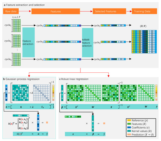
Figure 2.
The main framework of the proposed method. (a) Schematic of feature extraction and selection from cycle data consisting of time (t), voltage (v), current (I), and temperature (T). First, each cycle data matrix is condensed into a vector through feature extraction. Next, a subset is selected out of the original features using the MRMR algorithm. Finally, the raw cycle data matrix is transformed into a feature matrix, which is used as the input of the machine learning models. (b) Linear expression of Gaussian process regression. (c) Visualization of robust linear regression.
Considering the battery’s early aging process before capacity degradation, we used the cycle life indicator to describe the battery’s health state. The cycle life indicator is defined as
where is the current cycle number and is the total cycle number of the cycle test or the cycle number given by the battery manufacturers. The range of is from several hundred cycles to several thousand cycles due to various material and operation conditions.
As the cycle life of various cells is distinct, we defined the root-mean-square error (RMSE) and the mean absolute error (MAE) to metric the performance of the RLR and GPR models. The RMSE and MAE are defined as
where is the observed cycle number, is the predicted cycle number, is the total number of samples, and is the total cycle number of the cycle test or the cycle number given by the battery manufacturers.
4. Results
In this study, we explored two algorithms, robust linear regression (RLR) and Gaussian process regression (GPR), with three different datasets of lithium-ion batteries. First, we extracted 53 features based on raw discharge voltage curves. Second, we used the MRMR algorithm to select the top 20 features with the highest median scores as the feature subset to compare with the full feature set (53 features). The GPR algorithm and the RLR algorithm were deployed on the subset of features and on the full set of features, respectively. The results showed that all algorithms could accurately predict the battery cycle life with a low error. Specifically, RLR achieved a maximum average RMSE of 6.90% and a maximum average MAE of 4.77% for the selected feature subset, whereas the GPR model achieved a maximum average RMSE of 6.33% and a maximum average MAE of 3.91% for the same feature subset. The GPR algorithm exhibited greater prediction accuracy than the RLR algorithm, while the RLR algorithm demonstrated faster prediction speed than the GPR algorithm for both the full features and the feature subset.
4.1. Feature Extraction and Selection
Features were created on Datasets I through III. Figure 3 illustrates the typical features that were created on Dataset II. To the best of our knowledge, all features in Figure 3, except for skewness and kurtosis coefficients, were developed by us for the first time to predict the battery cycle life using machine learning methods. Most features in Figure 3 show some correlation with the cycle number. For instance, certain features, such as the zero-crossing rate, standard error, and mean frequency, increased as the cycle life increased. Conversely, features such as the root-sum-of-squares (RSS) level, Euclidean metric, absolute metric, and peak signal-to-noise ratio (PSNR) decreased as the cycle number increased. Furthermore, specific features, including the coefficient of skewness, root-mean-square (RMS) level, and band power, fluctuated over cycles during the first 100 cycles. However, despite most of the proposed features exhibiting a correlation with the cycle number, their values can greatly differ, varying by orders of magnitude, as illustrated in Figure 3.
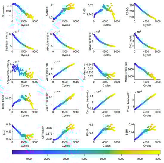
Figure 3.
Typical features of Dataset II.
Feature selection simplifies machine learning models, reduces overfitting, and improves model interpretability. The MRMR algorithm was selected to search for the optimal feature subset among the 53 pre-extracted features. The ranking of the features, arranged in descending order based on their median scores computed with the MRMR algorithm, is shown in Figure 4. Some of the new features from Figure 3, such as the mean frequency of the discharge voltage curve (dsgMeanFreq), the squared metric, and the Euclidean metric between the discharge voltage curve and the reference line (dsgDistSqr and dsgDistEucl), were among the top 20 features in the correlation ranking (as shown in Figure 4), indicating that the proposed features in Section 3 can serve as optimal inputs for machine learning models. Traditional features, such as total discharge capacity (dsgTotalAh), discharge voltage at the start (dsgVbegin), total discharge energy (dsgTotalWh), and discharge time (dsgTime), also had high scores, which is not unexpected, given their physical meaning associated with battery degradation. Additionally, numerical partial derivatives of voltage concerning the SOC (dsgDeltaV_dSOC80, dsgDeltaV_dSOC50, and dsgDeltaV_dSOC90 in Figure 4) were also found to be significant, confirming prior studies.
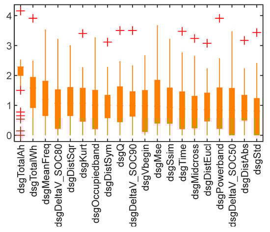
Figure 4.
Top 20 features ranked by the median of their scores according to the MRMR algorithm. The mark of “+” indicates an outlier.
The remaining features in Figure 4 are the kurtosis coefficient of the discharge voltage (dsgKurt), the discharge capacity (dsgQ), the occupied bandwidth of the discharge voltage curve (dsgOccupiedband), the symmetric Kullback–Leibler metric between the discharge voltage curve of cycle i and the reference line (dsgDistSym), the structural similarity index for the discharge voltage (dsgSsim), the mean square error between the discharge voltage of cycle i and the discharge voltage of the first cycle (dsgMse), the zero-crossing rate of the discharge voltage of cycle i (dsgZerorate), the band power of the discharge voltage of cycle i (dsgPowerband), the middle reference level for the discharge voltage of cycle i (dsgMidcross), the standard error between the discharge voltage of cycle i and the discharge voltage of the first cycle (dsgStd), and the Euclidean metric between the discharge voltage curve of cycle i and the reference line (dsgDistEucl).
The MRMR algorithm computes relevance scores for all features, while attempting to reduce redundancy. This study presented the use of the first 20 features as an example. However, determining the optimal number of features to use in practice depends on the requirements of accuracy in prediction and efficiency in computation for a particular field. Notably, the features based on discharge voltage proposed in this study are statistical analyses of the variations in the battery discharge voltage curve and may not have any practical physical significance.
4.2. Performance of Models Based on Full Features
To further evaluate the performance of our proposed method, we conducted a 5-fold cross-validation using two algorithms: Gaussian process regression (GPR) and robust linear regression (RLR). To validate the models’ performance on various load profiles and operating conditions, we assigned secondary test sets for all datasets. The training/testing partitions for Datasets I to III are summarized in Table 1. We tested the models using two feature sets: 53 features, which we named the full features, and a subset of the top 20 features selected using the maximum relevance minimum redundancy (MRMR) algorithm, which we referred to as the feature subset. The results demonstrated that both algorithms can accurately predict the battery cycle life with an error margin that is small compared to the actual cycle life, indicating that our proposed approach can yield reliable results and be used in applications that require accurate predictions of battery cycle life.

Table 1.
Selection and allocation of training and test datasets, including the charge protocols and discharge profiles.
The performance of the GPR and RLR algorithms on the full features of Datasets I-III is summarized in Table 2, Table 3 and Table 4. Both algorithms demonstrated promising performance across all datasets. The RLR algorithm achieved an average RMSE (ARMSE) of 6.90% and an average MAE (AMAE) of 4.77% on the test set of Dataset III, which was the model’s worst-case scenario. The GPR model’s worst performance was also observed on the test set of Dataset III, with an average RMSE and an average MAE of 6.33% and 3.91%, respectively. Figure 5, Figure 6 and Figure 7 provide a comparison between the predicted cycle life and the actual cycle life for the test batteries from Datasets I-III on the GPR and RLR algorithms.
Table 2.
Test results for the RLR and GPR models trained on the full feature set of Dataset I.
Table 3.
Test results for the RLR and GPR models trained on the full feature set of Dataset II.
Table 4.
Test results for the RLR and GPR models trained on the full feature set of Dataset III.
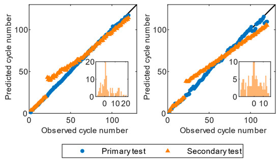
Figure 5.
Test results of the full feature models of Dataset I. The left plot shows the predictions of the GPR algorithm, and the right plot shows the predictions of the RLR algorithm. Cell 31 is the primary test set, and cell 32 is the secondary test set.
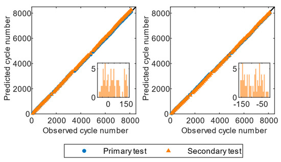
Figure 6.
Test results of the full feature models of Dataset II. The left plot shows the predictions of the GPR algorithm, and the right plot shows the predictions of the RLR algorithm. Cell 3 is the primary test set, and cell 4 is the secondary test set.
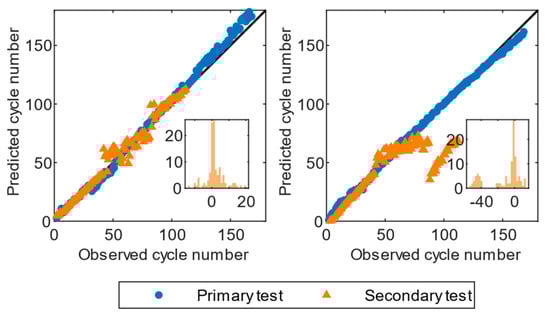
Figure 7.
Test results of the full feature models of Dataset III. The left plot shows the predictions of the GPR algorithm, and the right plot shows the predictions of the RLR algorithm. Cell 7 is the primary test set, and cell 44 is the secondary test set.
An interesting observation in the test set of Dataset I, as depicted in Figure 5, is the sudden fluctuation of predictions at approximately cycle 20. This notable rise can be attributed to the finding that the initial 20 cycles were characterized by a constant current discharge, whereas subsequent cycles were characterized by a random current discharge, resulting in considerable fluctuations in the prediction. Nevertheless, the GPR algorithm showed a gradual decrease in the residuals, eventually confining them to a small range. In contrast, RLR’s prediction diverged from the real cycle life after reaching a point of convergence, due to its limited ability to capture the nonlinearity of the degradation mechanisms. The predictions of cell 31 in Dataset I did not show any fluctuations near cycle 20, regardless of the analyzed GPR or RLR model, as cell 31 was cycled using the same constant current discharge profile.
It was evident that the RLR and GPR models achieved the best predictions in Dataset II, which contains cycle data from multiple batteries across all datasets. The average RMSE was 1.00% for the RLR algorithm and 1.03% for the GPR algorithm. Figure 6 illustrates that most predictions were near the diagonal, indicating a perfect match between the actual value and the predicted value. This result can largely be attributed to the finding that cells in Dataset II were cycled using the identical discharge profile. However, the distributions of residuals for GPR and RLR were distinct. As illustrated by the residual histograms in Figure 6, RLR exhibited a multimodal distribution, with all errors being negative, indicating that there may be several underlying sources of errors contributing to its overall performance. GPR had a moderately skewed distribution with a long rail to the right, and the largest peak was centered at zero, indicating that it was more prone to making large positive errors.
The predictions of the GPR and RLR models had a few outliers after cycle 50 during secondary testing in Dataset III, while the errors at primary testing were lower and did not present any outliers, as depicted in Figure 7.
The residual histograms of RLR in the secondary tests showed a few instances of large residuals at the tails of the distributions, suggesting that the model has difficulty handling certain extreme cases. The GPR model had a roughly bell-shaped distribution with a high peak at approximately zero, indicating that the model is better at capturing than RLR.
Overall, the GPR algorithm trained on Datasets I, II, and III is suggested to be more accurate in the tests, as it achieved lower relative MAE values and, in most cases, lower RMSE values compared to those of the RLR algorithm. However, there was an exception in the primary test of Dataset II, where RLR achieved an average RMSE of 1.00%, which was lower than GPR’s RMSE of 1.03%. This result may be attributed to the discharge profile of cells in Dataset II being the same during the cycle test.
4.3. Performance of Models Based on Feature Subsets
We also explored GPR and RLR algorithms using 20 selected features (as shown in Figure 4). Table 5, Table 6 and Table 7 summarize the test results of the GPR and RLR algorithms. Figure 8, Figure 9 and Figure 10 illustrate the battery cycle life predictions versus observations and the residual histograms based on 20 features from Datasets I-III. Both GPR and RLR exhibited lower prediction errors on all datasets. Specifically, RLR achieved an average RMSE of 0.75% and an average MAE of 0.52% on Dataset II. In contrast, GPR achieved an average RMSE and MAE of 0.67% and 0.54%, respectively, on the same dataset, indicating that GPR outperforms RLR on Dataset II. GPR also performed better than RLR on the other two datasets.
Table 5.
Test results for the RLR and GPR models trained on the feature subset of Dataset I.
Table 6.
Test results for the RLR and GPR models trained on the feature subset of Dataset II.
Table 7.
Test results for the RLR and GPR models trained on the feature subset of Dataset III.
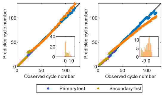
Figure 8.
Test results of the feature subset models of Dataset I. The left plot shows the predictions of the GPR algorithm, and the right plot shows the predictions of the RLR algorithm. Cell 31 is the primary test set, and cell 32 is the secondary test set.
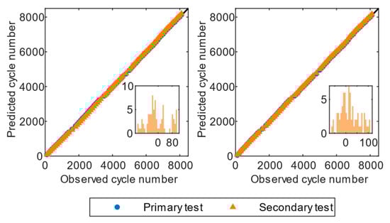
Figure 9.
Test results of the feature subset models of Dataset II. The left plot shows the predictions of the GPR algorithm, and the right plot shows the predictions of the RLR algorithm. Cell 3 is the primary test set, and cell 7 is the secondary test set.
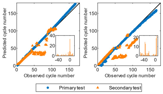
Figure 10.
Test results of the full feature models of Dataset III. The left plot shows the predictions of the GPR algorithm, and the right plot shows the predictions of the RLR algorithm. Cell 7 is the primary test set, and cell 44 is the secondary test set.
Both GPR and RLR achieved an average RMSE and MAE of less than 3.4%. Comparing the residual histograms of the two algorithms on feature subsets of Dataset I, we discovered that GPR has a more negatively skewed distribution with a right tail, indicating that GPR is more likely to have positive errors. Conversely, the residual histogram of RLR showed a positively skewed distribution with a left tail, indicating that RLR is prone to having negative errors. Comparing the test results of the full features on the same dataset, we discovered that both GPR and RLR based on feature subsets output more accurate predictions than those based on full features (Table 2).
Cells in Dataset II were cycled with the ARTEMIS dynamic driving profile, followed by characterization cycles. It is evident from Figure 6 and Figure 9 that the performance of tests in Dataset II was dominated by RLR, according to both RMSE and MAE. The largest RMSE achieved by both models was 0.89%, which is less than that of Dataset I. The cells in Dataset II had been cycled up to 8000 cycles, and both GPR and RLR achieved an average RMSE and MAE of less than 0.75% of the entire cycle life. Table 3 and Table 6 show that both models based on feature subsets outperformed the models based on the full features of Dataset II, indicating that feature selection by MRMR could improve the prediction accuracy on the dataset. The high performance achieved by GPR and RLR in Dataset II may be attributed to the low variability in the charge and discharge conditions.
Both GPR and RLR based on feature subsets of Dataset III achieved the highest RMSE and MAE across all datasets. Both histograms of the residuals of GPR in Figure 7 and Figure 10 show skewed distributions. Specifically, GPR on full features showed a negatively skewed distribution with a long tail to the right, and the peak center was approximately zero, indicating that it is prone to outputting positive errors. Conversely, GPR on feature subsets exhibited a positively skewed distribution with a long tail to the left, and the peak center was also approximately zero, indicating that it is prone to having negative errors. The residuals of RLR exhibited a multimodal distribution on the feature subset, indicating that there may be several underlying sources of errors contributing to its overall performance. The residual histogram of RLR on full features also showed two peaks, but the second peak was lower than that of RLR on the feature subset. GPR and RLR on the feature subset achieved a lower average RMSE and MAE than those on full features, suggesting that the feature selection could avoid overfitting.
The prediction speed of the two algorithms on both full features and feature subsets of Datasets I to III are summarized in Table 8. All models were trained and tested on a computer with two Intel Xeon 2666 V3 CPUs and an Nvidia 2080Ti GPU.
Table 8.
Training time and prediction speed of the full feature models and feature subset models.
As expected, the feature subset models showed a significantly higher prediction speed than the full feature models, primarily due to a reduction of more than half of the variables. RLR particularly emphasized this point, demonstrating a minimum of twice the prediction speed of the full feature set models, except for Dataset I, which showed an almost 50% faster prediction speed. For GPR, all three datasets showed an increase in the prediction speed of less than 50%, except for Dataset II. This discrepancy is attributed to the complex random process of the GPR algorithm, which impacts the overall prediction speed.
The results of using feature subsets, instead of full features, in GPR for Dataset I yielded considerable reductions in training time. Conversely, for Datasets II and III, the difference in training time between the models using feature subsets and full features was limited to 2 s. As Table 1 describes, Dataset I consists of most cells of the three datasets, so the training time of GPR was the largest, with a maximum of 372.840 s. The training time of GPR for Datasets II and III was smaller than that of GPR for Dataset I, and the training speed of the two algorithms did was not significantly improve.
5. Discussion
The proposed battery cycle life prediction approach promises to enhance battery management systems, allowing for highly accurate estimation of battery degradation. This proposed method is distinct in that it can estimate cycle life using only discharge voltage curves and can accommodate various operational conditions, such as random or high discharge rates. Future work could be extended to random partial discharge/charge scenarios and batteries with different designs and chemistries.
The algorithms based on full features had strong performance, as they achieved a low RMSE and MAE, but the large feature set was too complicated for onboard application and likely contained some redundancies. To address this issue, we used the MRMR algorithm for feature selection. The score distribution of each feature indicated that the importance of features is not consistent across the different datasets. This lack of consistency could be attributed to the various aging mechanisms and modes present in the different battery datasets, which were caused by the varying cycle conditions and charge/discharge protocols. Therefore, it is essential to select features using the MRMR algorithm for each respective battery dataset prior to model training to achieve a satisfactory trade-off between accuracy and computational efficiency.
To meet real-time requirements, a subset of 20 features was selected from 53 features as a paradigm of feature selection; these features could be extracted from every cycle discharge profile. The aim of the proposed method was to optimize a process suitable for on-board applications that emphasize computation efficiency and real-time accuracy over precision. Therefore, multicycle features were excluded, as they require the extraction of multiple cycle data, and we used only features that can be calculated for each cycle.
Our investigation of two algorithms, GPR and RLR, for three datasets revealed that feature selection has a positive effect on the performance of both algorithms for Datasets I and III, except for Dataset II. Specifically, both algorithms achieved relatively low average RMSEs and MAEs for all datasets, and GPR outperformed RLR in terms of RMSE and MAE for both feature subsets and full features of Datasets I and III, indicating that GPR is the optimal algorithm for large battery datasets with complex discharge profiles. Conversely, RLR output accurate predictions with a lower RMSE and MAE for Dataset II compared to GPR, owing to identical discharge profiles. As discussed in Section 3, lithium-ion battery aging is a nonlinear process with a multitude of potential factors. It can be seen from Figure 4 that almost all features demonstrate nonlinear correlations with the cycle number. The GPR model incorporates a nonlinear kernel function, which is used to fit the correlation between input and target. This kernel function makes GPR perform better than RLR for battery cycle life prediction, especially under dynamic load profiles.
Table 9 compared the proposed method and 10 different data-driven methods for battery degradation estimation. Compared to previous methods, we developed some new features, such as the warp distance of discharge voltages, which makes it possible to extract useful information from dynamic discharge profiles. The main reason for the discrepancy in results between our methods and those of other literature can be attributed to the difference in targets of machine learning models. As seen in Table 9, our model uses the cycle life index (CI) as the target, the denominator of which is the total cycle number of the cycle tests. In contrast, the equation of the remaining useful life (RUL) reported by other literature has a different denominator, namely the cycle life given by the manufacturer. For instance, in Dataset III, the total cycle number of tests averages 131 cycles, while the cycle life given by the manufacturer ranges between 300 and 500 cycles. The difference in denominators of the targets thus affects the RMSE of the two methods. Another reason for the discrepancy in the results between our methods and other methods is the use of a linear regression model, which is less accurate than other machine learning algorithms in dynamic load profiles. Training linear regression models requires less computational resources than most machine learning models, and it is simple to implement linear regression models, which makes it possible to apply machine learning algorithms to onboard battery management systems in electric vehicles. Many studies [1,8,31,32] have demonstrated that linear regression is good at fitting simple battery degradation with minimal variance in charge and discharge conditions. After considering both the prediction speed and the training cost, we determined that the RLR algorithm is optimal for battery life estimation in onboard applications with inadequate computing resources and high real-time requirements, whereas the GPR algorithm is better suited for battery pack manufacturing and recycling, due to the high prediction accuracy requirements and sufficient computational power.
Table 9.
Comparison of various data-driven methods for battery degradation estimation.
6. Conclusions
Data-driven models are widely adopted for diagnosing and prognosticating the behavior of lithium-ion batteries. In this study, we proposed a data-driven framework to accurately predict battery cycle life using various discharge profiles. This method offers several advantages over conventional methods, including adaptability to random and high discharge rates, robustness to changes in discharge mode, and prediction based solely on discharge profiles.
We extracted 53 features from battery discharge profiles, 18 of which were newly proposed for battery cycle life prediction models. The MRMR algorithm was used for feature selection. We explored two machine learning models: GPR and RLR. All models were evaluated using the error metrics RMSE and MAE. GPR achieved a maximum RMSE of 6.33% and a maximum MAE of 3.91%, while RLR attained a maximum RMSE of 6.90% and a maximum MAE of 4.77%. GPR was preferred for battery pack manufacturing and recycling, while RLR was preferred for on-board battery cycle life prediction.
Overall, our work highlights the value of combining machine learning techniques with discharge profiles for battery cycle life estimation. Moreover, although the estimation accuracy is not always improved, the algorithm should be subjected to feature selection before being deployed in the field. We demonstrate that feature selection can improve the prediction accuracy and reduce the computational cost. We infer that this framework should also be effective with charge profiles. In future work, it would be beneficial to combine features extracted from both charge profiles and discharge profiles and to use this method to prognosticate batteries with different materials.
Author Contributions
Conceptualization, Y.J. and W.S.; methodology, Y.J.; software, Y.J.; validation, Y.J.; formal analysis, Y.J.; investigation, Y.J.; resources, Y.J.; data curation, Y.J.; writing—original draft preparation, Y.J.; writing—review and editing, W.S.; visualization, Y.J.; supervision, W.S.; project administration, Y.J.; funding acquisition, W.S. All authors have read and agreed to the published version of the manuscript.
Funding
This research received no external funding.
Data Availability Statement
The battery datasets used in this study are available at https://data.mendeley.com/datasets/kw34hhw7xg (accessed on 4 August 2023) for Dataset I, https://ora.ox.ac.uk/objects/uuid:03ba4b01-cfed-46d3-9b1a-7d4a7bdf6fac (accessed on 4 August 2023) for Dataset II, and https://phmdatasets.s3.amazonaws.com/NASA/5.+Battery+Data+Set.zip for Dataset III (accessed on 4 August 2023).
Conflicts of Interest
The authors declare no conflict of interest.
References
- Roman, D.; Saxena, S.; Robu, V.; Pecht, M.; Flynn, D. Machine Learning Pipeline for Battery State-of-Health Estimation. Nat. Mach. Intell. 2021, 3, 447–456. [Google Scholar] [CrossRef]
- Ng, M.-F.; Zhao, J.; Yan, Q.; Conduit, G.J.; Seh, Z.W. Predicting the State of Charge and Health of Batteries Using Data-Driven Machine Learning. Nat. Mach. Intell. 2020, 2, 161–170. [Google Scholar] [CrossRef]
- Tran, M.-K.; Mathew, M.; Janhunen, S.; Panchal, S.; Raahemifar, K.; Fraser, R.; Fowler, M. A Comprehensive Equivalent Circuit Model for Lithium-Ion Batteries, Incorporating the Effects of State of Health, State of Charge, and Temperature on Model Parameters. J. Energy Storage 2021, 43, 103252. [Google Scholar] [CrossRef]
- Weng, C.; Sun, J.; Peng, H. A Unified Open-Circuit-Voltage Model of Lithium-Ion Batteries for State-of-Charge Estimation and State-of-Health Monitoring. J. Power Sources 2014, 258, 228–237. [Google Scholar] [CrossRef]
- Bian, X.; Liu, L.; Yan, J.; Zou, Z.; Zhao, R. An Open Circuit Voltage-Based Model for State-of-Health Estimation of Lithium-Ion Batteries: Model Development and Validation. J. Power Sources 2020, 448, 227401. [Google Scholar] [CrossRef]
- Bian, X.; Wei, Z.; Li, W.; Pou, J.; Sauer, D.U.; Liu, L. State-of-Health Estimation of Lithium-Ion Batteries by Fusing an Open Circuit Voltage Model and Incremental Capacity Analysis. IEEE Trans. Power Electron. 2022, 37, 2226–2236. [Google Scholar] [CrossRef]
- Li, J.; Adewuyi, K.; Lotfi, N.; Landers, R.G.; Park, J. A Single Particle Model with Chemical/Mechanical Degradation Physics for Lithium Ion Battery State of Health (SOH) Estimation. Appl. Energy 2018, 212, 1178–1190. [Google Scholar] [CrossRef]
- Severson, K.A.; Attia, P.M.; Jin, N.; Perkins, N.; Jiang, B.; Yang, Z.; Chen, M.H.; Aykol, M.; Herring, P.K.; Fraggedakis, D.; et al. Data-Driven Prediction of Battery Cycle Life before Capacity Degradation. Nat. Energy 2019, 4, 383–391. [Google Scholar] [CrossRef]
- Ma, Z.; Yang, R.; Wang, Z. A Novel Data-Model Fusion State-of-Health Estimation Approach for Lithium-Ion Batteries. Appl. Energy 2019, 237, 836–847. [Google Scholar] [CrossRef]
- Deng, Z.; Hu, X.; Li, P.; Lin, X.; Bian, X. Data-Driven Battery State of Health Estimation Based on Random Partial Charging Data. IEEE Trans. Power Electron. 2022, 37, 5021–5031. [Google Scholar] [CrossRef]
- Zhu, J.; Wang, Y.; Huang, Y.; Bhushan Gopaluni, R.; Cao, Y.; Heere, M.; Mühlbauer, M.J.; Mereacre, L.; Dai, H.; Liu, X.; et al. Data-Driven Capacity Estimation of Commercial Lithium-Ion Batteries from Voltage Relaxation. Nat. Commun. 2022, 13, 2261. [Google Scholar] [CrossRef] [PubMed]
- Zhang, Y.; Tang, Q.; Zhang, Y.; Wang, J.; Stimming, U.; Lee, A.A. Identifying Degradation Patterns of Lithium Ion Batteries from Impedance Spectroscopy Using Machine Learning. Nat. Commun. 2020, 11, 1706. [Google Scholar] [CrossRef]
- Vermeer, W.; Chandra Mouli, G.R.; Bauer, P. A Comprehensive Review on the Characteristics and Modeling of Lithium-Ion Battery Aging. IEEE Trans. Transp. Electrif. 2022, 8, 2205–2232. [Google Scholar] [CrossRef]
- Tian, H.; Qin, P.; Li, K.; Zhao, Z. A Review of the State of Health for Lithium-Ion Batteries: Research Status and Suggestions. J. Clean. Prod. 2020, 261, 120813. [Google Scholar] [CrossRef]
- Shahjalal, M.; Roy, P.K.; Shams, T.; Fly, A.; Chowdhury, J.I.; Ahmed, M.R.; Liu, K. A Review on Second-Life of Li-Ion Batteries: Prospects, Challenges, and Issues. Energy 2022, 241, 122881. [Google Scholar] [CrossRef]
- Chen, M.; Ma, G.; Liu, W.; Zeng, N.; Luo, X. An Overview of Data-Driven Battery Health Estimation Technology for Battery Management System. Neurocomputing 2023, 532, 152–169. [Google Scholar] [CrossRef]
- Vanem, E.; Salucci, C.B.; Bakdi, A.; Sheim Alnes, Ø.Å. Data-Driven State of Health Modelling—A Review of State of the Art and Reflections on Applications for Maritime Battery Systems. J. Energy Storage 2021, 43, 103158. [Google Scholar] [CrossRef]
- Che, Y.; Hu, X.; Lin, X.; Guo, J.; Teodorescu, R. Health Prognostics for Lithium-Ion Batteries: Mechanisms, Methods, and Prospects. Energy Environ. Sci. 2023, 16, 338–371. [Google Scholar] [CrossRef]
- Sui, X.; He, S.; Vilsen, S.B.; Meng, J.; Teodorescu, R.; Stroe, D.-I. A Review of Non-Probabilistic Machine Learning-Based State of Health Estimation Techniques for Lithium-Ion Battery. Appl. Energy 2021, 300, 117346. [Google Scholar] [CrossRef]
- Jiang, S.; Song, Z. A Review on the State of Health Estimation Methods of Lead-Acid Batteries. J. Power Sources 2022, 517, 230710. [Google Scholar] [CrossRef]
- Li, Y.; Stroe, D.-I.; Cheng, Y.; Sheng, H.; Sui, X.; Teodorescu, R. On the Feature Selection for Battery State of Health Estimation Based on Charging–Discharging Profiles. J. Energy Storage 2021, 33, 102122. [Google Scholar] [CrossRef]
- Luo, K.; Chen, X.; Zheng, H.; Shi, Z. A Review of Deep Learning Approach to Predicting the State of Health and State of Charge of Lithium-Ion Batteries. J. Energy Chem. 2022, 74, 159–173. [Google Scholar] [CrossRef]
- Deng, Z.; Hu, X.; Lin, X.; Xu, L.; Che, Y.; Hu, L. General Discharge Voltage Information Enabled Health Evaluation for Lithium-Ion Batteries. IEEE/ASME Trans. Mechatron. 2021, 26, 1295–1306. [Google Scholar] [CrossRef]
- Messing, M.; Shoa, T.; Habibi, S. Estimating Battery State of Health Using Electrochemical Impedance Spectroscopy and the Relaxation Effect. J. Energy Storage 2021, 43, 103210. [Google Scholar] [CrossRef]
- Pradhan, S.K.; Chakraborty, B. Battery Management Strategies: An Essential Review for Battery State of Health Monitoring Techniques. J. Energy Storage 2022, 51, 104427. [Google Scholar] [CrossRef]
- Paulson, N.H.; Kubal, J.; Ward, L.; Saxena, S.; Lu, W.; Babinec, S.J. Feature Engineering for Machine Learning Enabled Early Prediction of Battery Lifetime. J. Power Sources 2022, 527, 231127. [Google Scholar] [CrossRef]
- Gou, B.; Xu, Y.; Feng, X. State-of-Health Estimation and Remaining-Useful-Life Prediction for Lithium-Ion Battery Using a Hybrid Data-Driven Method. IEEE Trans. Veh. Technol. 2020, 69, 10854–10867. [Google Scholar] [CrossRef]
- Zhou, Z.; Duan, B.; Kang, Y.; Shang, Y.; Cui, N.; Chang, L.; Zhang, C. An Efficient Screening Method for Retired Lithium-Ion Batteries Based on Support Vector Machine. J. Clean. Prod. 2020, 267, 121882. [Google Scholar] [CrossRef]
- Zhang, J.; Wang, P.; Gong, Q.; Cheng, Z. SOH Estimation of Lithium-Ion Batteries Based on Least Squares Support Vector Machine Error Compensation Model. J. Power Electron. 2021, 21, 1712–1723. [Google Scholar] [CrossRef]
- Li, R.; Li, W.; Zhang, H. State of Health and Charge Estimation Based on Adaptive Boosting Integrated with Particle Swarm Optimization/Support Vector Machine (AdaBoost-PSO-SVM) Model for Lithium-Ion Batteries. Int. J. Electrochem. Sci. 2022, 17, 220212. [Google Scholar] [CrossRef]
- Shi, M.; Xu, J.; Lin, C.; Mei, X. A Fast State-of-Health Estimation Method Using Single Linear Feature for Lithium-Ion Batteries. Energy 2022, 256, 124652. [Google Scholar] [CrossRef]
- Vilsen, S.B.; Stroe, D.-I. Battery State-of-Health Modelling by Multiple Linear Regression. J. Clean. Prod. 2021, 290, 125700. [Google Scholar] [CrossRef]
- Lu, J.; Xiong, R.; Tian, J.; Wang, C.; Hsu, C.-W.; Tsou, N.-T.; Sun, F.; Li, J. Battery Degradation Prediction against Uncertain Future Conditions with Recurrent Neural Network Enabled Deep Learning. Energy Storage Mater. 2022, 50, 139–151. [Google Scholar] [CrossRef]
- Ma, G.; Xu, S.; Jiang, B.; Cheng, C.; Yang, X.; Shen, Y.; Yang, T.; Huang, Y.; Ding, H.; Yuan, Y. Real-Time Personalized Health Status Prediction of Lithium-Ion Batteries Using Deep Transfer Learning. Energy Environ. Sci. 2022, 15, 4083–4094. [Google Scholar] [CrossRef]
- Wang, Z.; Yuan, C.; Li, X. Lithium Battery State-of-Health Estimation via Differential Thermal Voltammetry With Gaussian Process Regression. IEEE Trans. Transp. Electrific. 2021, 7, 16–25. [Google Scholar] [CrossRef]
- Guo, W.; Sun, Z.; Vilsen, S.B.; Meng, J.; Stroe, D.I. Review of “Grey Box” Lifetime Modeling for Lithium-Ion Battery: Combining Physics and Data-Driven Methods. J. Energy Storage 2022, 56, 105992. [Google Scholar] [CrossRef]
- Birkl, C.R.; Roberts, M.R.; McTurk, E.; Bruce, P.G.; Howey, D.A. Degradation Diagnostics for Lithium Ion Cells. J. Power Sources 2017, 341, 373–386. [Google Scholar] [CrossRef]
- André, M. The ARTEMIS European Driving Cycles for Measuring Car Pollutant Emissions. Sci. Total Environ. 2004, 334–335, 73–84. [Google Scholar] [CrossRef]
- Goebel, K.; Saha, B.; Saxena, A.; Celaya, J.; Christophersen, J. Prognostics in Battery Health Management. IEEE Instrum. Meas. Mag. 2008, 11, 33–40. [Google Scholar] [CrossRef]
- Xiong, R.; Pan, Y.; Shen, W.; Li, H.; Sun, F. Lithium-Ion Battery Aging Mechanisms and Diagnosis Method for Automotive Applications: Recent Advances and Perspectives. Renew. Sustain. Energy Rev. 2020, 131, 110048. [Google Scholar] [CrossRef]
- Peng, H.; Long, F.; Ding, C. Feature Selection Based on Mutual Information Criteria of Max-Dependency, Max-Relevance, and Min-Redundancy. IEEE Trans. Pattern Anal. Mach. Intell. 2005, 27, 1226–1238. [Google Scholar] [CrossRef] [PubMed]
- Zhao, Z.; Anand, R.; Wang, M. Maximum Relevance and Minimum Redundancy Feature Selection Methods for a Marketing Machine Learning Platform. In Proceedings of the 2019 IEEE International Conference on Data Science and Advanced Analytics (DSAA), Washington, DC, USA, 5–8 October 2019. [Google Scholar]
- Lin, M.; Zeng, X.; Wu, J. State of Health Estimation of Lithium-Ion Battery Based on an Adaptive Tunable Hybrid Radial Basis Function Network. J. Power Sources 2021, 504, 230063. [Google Scholar] [CrossRef]
- Weng, A.; Mohtat, P.; Attia, P.M.; Sulzer, V.; Lee, S.; Less, G.; Stefanopoulou, A. Predicting the Impact of Formation Protocols on Battery Lifetime Immediately after Manufacturing. Joule 2021, 5, 2971–2992. [Google Scholar] [CrossRef]
Disclaimer/Publisher’s Note: The statements, opinions and data contained in all publications are solely those of the individual author(s) and contributor(s) and not of MDPI and/or the editor(s). MDPI and/or the editor(s) disclaim responsibility for any injury to people or property resulting from any ideas, methods, instructions or products referred to in the content. |
© 2023 by the authors. Licensee MDPI, Basel, Switzerland. This article is an open access article distributed under the terms and conditions of the Creative Commons Attribution (CC BY) license (https://creativecommons.org/licenses/by/4.0/).