A Novel Fine-Tuning Model Based on Transfer Learning for Future Capacity Prediction of Lithium-Ion Batteries

Abstract

Future capacity prediction of lithium-ion batteries is a highly researched topic in the field of battery management systems, owing to the gradual degradation of battery capacity over time due to various factors such as chemical changes within the battery, usage patterns, and operating conditions. The accurate prediction of battery capacity can aid in optimizing its usage, extending its lifespan, and mitigating the risk of unforeseen failures. In this paper, we proposed a novel fine-tuning model based on a deep learning model with a transfer learning approach comprising of two key components: offline training and online prediction. Model weights and prediction parameters were transferred from offline training using source data to the online prediction stage. The transferred Bi-directional Long Short-Term Memory with an Attention Mechanism model weights and prediction parameters were utilized to fine-tune the model by partial target data in the online prediction phase. Three battery batches with different charging policy were used to evaluate the proposed approach’s robustness, reliability, usability, and accuracy for the three charging policy batteries’ real-world data. The experiment results show that the proposed method’s efficacy improved, with an increase in the cycle number of the starting point, exhibiting a linear relationship with the starting point. The proposed method yields relative error values of 8.70%, 6.38%, 9.52%, 7.58%, 1.94%, and 2.29%, respectively, for the six target batteries in online prediction. Thus, the proposed method is effective in predicting the future capacity of lithium-ion batteries and holds potential for use in predictive maintenance applications.

1. Introduction

Lithium-ion (Li-ion) batteries have several applications in different areas, including electric vehicles, autonomous mobile robots, automatic guided vehicles, portable electronics, and renewable energy systems. The mobile devices’ service time depends on the battery’s State of Health (SOH), which can represent the batteries’ working available period, long or short [1]. The ability to estimate how much energy a Li-ion battery will be able to store and deliver over time, based on various factors such as usage patterns, temperature, charging and discharging rates, and the age of the battery has become an important issue [2,3,4,5,6]. Forecasting the future capacity of batteries and their Remaining Useful Life (RUL) represents a complex issue within the domain of battery health diagnosis and management applications [7,8].

To the best of our knowledge, a majority of studies do not provide comprehensive explanations on the training approach and training data generation procedures for input and output data utilized in training data-driven models, including machine learning and deep learning models implemented through sliding window approach. Additionally, only a limited number of studies have directly captured long-term dynamics and local regeneration within this context. The authors of [4] combined the advantages of Long Short-Term Memory (LSTM) and Gaussian Process Regression for future capacity and RUL prediction. One of the challenges in predicting the RUL of batteries is the use of unknown data, where data beyond the starting point of RUL prediction are unavailable. Consequently, research in this area is complex, and only a limited number of studies have been published on the subject. To enhance the accuracy of RUL predictions and solve the lack of run-to-failure data problem, one effective approach is the use of Transfer Learning (TL) method. The TL method involves transferring the knowledge learned from a pre-trained model, trained on a source dataset, to a target dataset with a similar structure. By leveraging the existing knowledge, the TL method can reduce the amount of training data required, improve the generalization performance of the model, and enhance the accuracy of RUL predictions. The transfer learning approach can be applied to different types of machine learning models, including deep learning models, and has shown promising results in predicting the RUL of Li-ion batteries [9,10,11]. TL involves training a base model using a source dataset and subsequently transferring the learned parameters to a target model using a target dataset, following fine-tuning of the learned parameters.

The advance of machine learning and deep learning increased the application of data-driven methods for RUL prediction [4]. Although data-driven methods offer a cost-effective and straightforward alternative to model-based methods, the significant amount of data required for achieving accurate prediction performance poses a challenge for their widespread application. To address this challenge, TL has emerged as one of the strategies for mitigating the issue of limited data for analysis. The TL approach involves training a base model using a base dataset and subsequently transferring the learned parameters to a target model trained with a target dataset, following fine-tuning of the learned parameters. This method allows for effective knowledge transfer and can improve the generalization performance of the model [12,13,14,15,16,17,18].

Accurately predicting the online RUL of batteries is crucial in battery management systems utilized in industrial applications. Throughout the battery’s life cycle, side reactions lead to a decline in its capacity and internal resistance. Moreover, battery systems necessitate reliable and precise battery health diagnostics, timely maintenance, and replacement. While many published algorithms for Li-ion battery RUL prediction employ offline methods, these unmodified prediction results provided by offline approaches cannot monitor the overall trend in changes, resulting in lower accuracy. This poses a significant challenge for the widespread use of smart Battery Management Systems (BMS). Despite studies on the application of TL for Li-ion battery RUL prediction, most previously published papers do not discuss the training start point, or they choose a random starting point for model training. Therefore, improving the accuracy of prediction methods remains a critical task in enhancing the efficiency of smart BMS [19].

This study presents an online RUL prediction method for effective battery health management, utilizing a Bi-directional Long Short-Term Memory with an Attention Mechanism (BiLSTM-AT) model. The proposed approach leverages the TL technique to enhance the accuracy of Li-ion battery RUL prediction, incorporating fixed-length training data points and a knee-onset point concept for the prediction starting point.

The main objective of this study is to propose a fine-tuning model based on TL as an accurate online RUL approach for improved prognostics and health management. The specific contributions of this study are:

• Through the implementation of a fine-tuning model, it becomes feasible to showcase the utilization of TL as a solution to the challenge of data paucity, via the transference of pre-trained weights from a source dataset to a target dataset.
• To provide a detailed explanation of the strategy for fine-tuning a transferred model in order to adapt it to the source data: This involves adjusting the pre-trained model’s parameters to improve its performance on the specific task and dataset it is being applied to. The process of fine-tuning enables the model to learn new information and patterns that are specific to the source data, while still retaining its knowledge gained from the pre-training stage.
• Through the utilization of the sliding window methodology to obtain a multi-step-ahead prediction of future capacity, it is viable to significantly augment the precision of prognostications for Li-ion battery.
• To showcase a hybrid loss function that can be used to evaluate the performance of a data-driven model during the optimization of both hyperparameters and prediction parameters: The loss function combines multiple criteria for assessing the model’s performance, such as accuracy, precision, recall, and F1 score, into a single objective function that can be optimized using gradient-based methods. By using a hybrid loss function, it becomes possible to consider multiple performance metrics simultaneously and to balance the trade-offs between them during optimization.

The rest of this paper is organized as follows. Section 2 is a literature review of RUL prediction, TL, and knee point and knee onset concepts. Section 3 presents the research methods, including the sliding window method, transferability measurement, BiLSTM-AT and performance evaluation metrics. The results of the transfer learning approach for the Li-ion battery are presented in Section 4. Finally, we draw conclusions in Section 5.

2. Related Works

In our study, we define the RUL of a battery as the cycle life between the present cycle number and the end of the battery’s useful life. This means that RUL represents the number of additional cycles that the battery is expected to be able to complete before it reaches the end of its lifespan. We formalize this definition using Equation (1), which provides a mathematical expression for RUL based on the present cycle number and the total cycle life of the battery.

RUL_t = t_EOL − t_sp,

(1)

where t_sp is the starting cycle number for RUL prediction, RUL_t is the remaining life at t_sp, and t_EOL is the end of life. In addition, SOH is given by the normalization of charge/discharge capacity, that is SOH = C_t/C₀, where C_t is the current capacity and C₀ is the rated capacity.

Li-ion cells exhibit different capacity degradation trends until their EOL. However, there will be a slow capacity degradation trend up to a certain point; after this point, there will be accelerated capacity degradation up to the EOL. This point where the capacity trend changes from slow degradation to rapid one is known as knee point. The knee point can be an informative indicator of more severe battery degradation trends and a signal to indicate when battery replacements should be scheduled and when secondary uses of the battery should be considered.

Different researchers define the knee point in different ways. The knee point is defined as the point of intersection of two tangent lines on the capacity fade curve [20]. They define the knee point as of two tangent lines on the capacity fade curve. They found the cycle number of the intersection of the tangent lines by assessing the slop-changing ratio of capacity fade curve. The authors of [21] treated the knee point as a point where two lines intersect at the knee point that represent two different signs of capacity degradation. They proposed a method to identify the knee point for capacity fade curve and introduced the concept of knee-onset based on a double Bacon–Watts model which indicate the beginning of nonlinear degradation. This knee-onset concept will provide an earlier warning than the knee point where the rapid degradation is already in progress. An elbow point and elbow-onset identification algorithm for Internal Resistance (IR) rise curves based on knee point and knee-onset identification concepts for capacity degradation curves was devised in [22]. Their study found out that there is a significant linear relationship between end of life, knee point of capacity (elbow point of IR), and knee-onset of capacity (elbow onset of IR) for a large dataset of lithium-ion batteries. The authors of [23] also considered the knee point effect to predict the future ageing trajectory for Li-ion batteries.

In this study, the concept of knee-onset was applied to determine the RUL prediction starting point. The double Bacon and Watts model was adopted to identify the RUL prediction starting point for the transfer learning approach, indicating the beginning of nonlinear degradation.

γ = α₀ +α₁(x − x₀) +α₂(x − x₀)tanh{(x − x₀)/γ} + α₃(x − x₂)tanh{(x − x₂)/γ} + z,

(2)

where z represents the residual, α_i and x_j are the parameters to be estimated, and γ is a fixed small value to get a rapid change around the points x₀, and x₂. Equation (2) is known as the double Bacon–Watts model. The transition point x₀ in the fitted results is defined as the knee-onset point.

3. Proposed Method

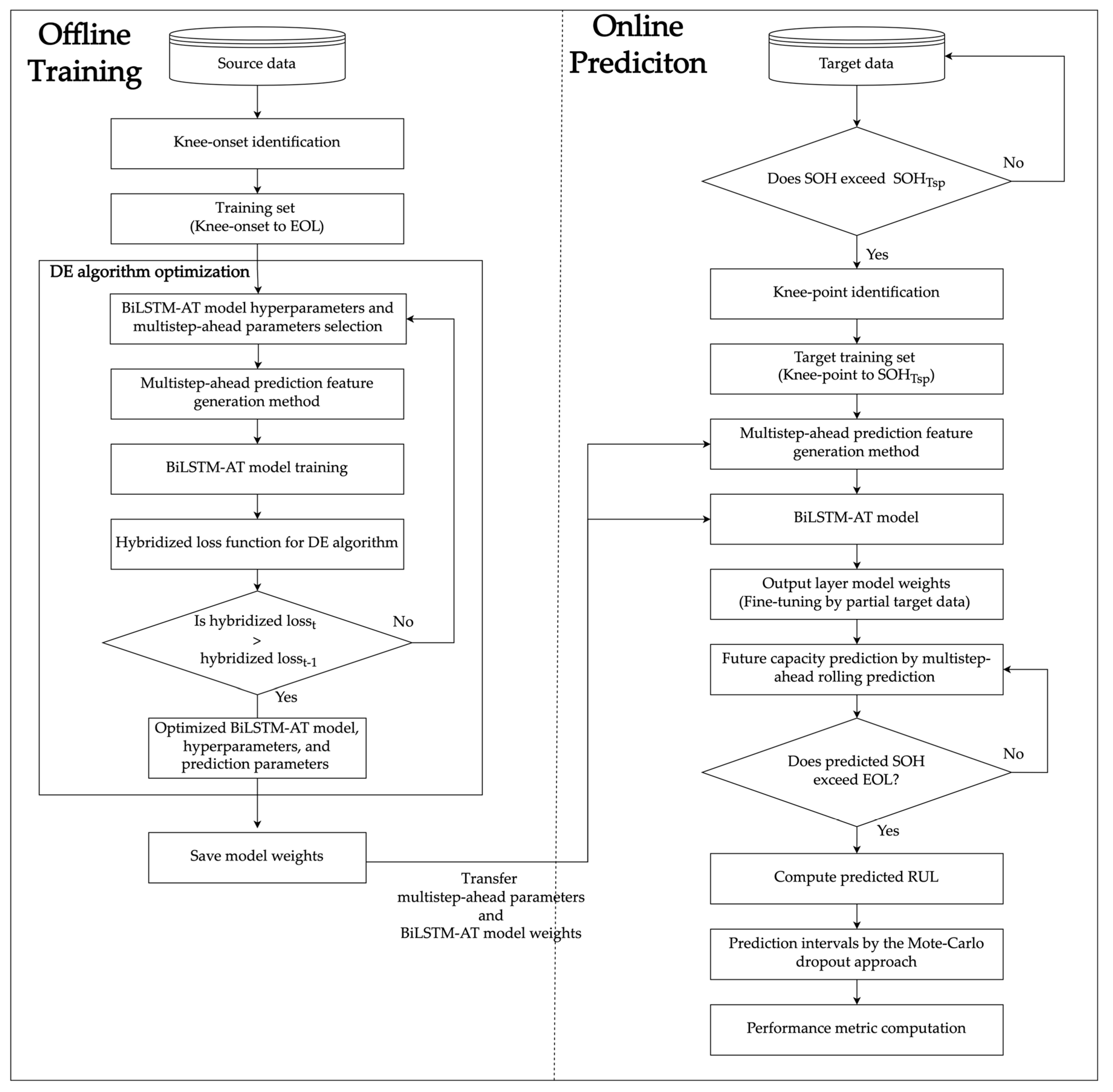
The proposed method can be divided into two parts, which are offline training and online prediction. We transferred the model weights and prediction parameters from offline training using source data to the online prediction. The transferred BiLSTM-AT model weights and prediction parameters were used to fine-tune the model weights by partial target data in the online prediction. Figure 1 shows the proposed method flowchart.

In offline training, the double Bacon–Watts model selects the knee-onset point that marks the onset of the SOH accelerated degradation rate. To train the model more efficiently, we define the training data from the cycle of knee-onset to the last of the source SOH data, namely SOH_tEOL. 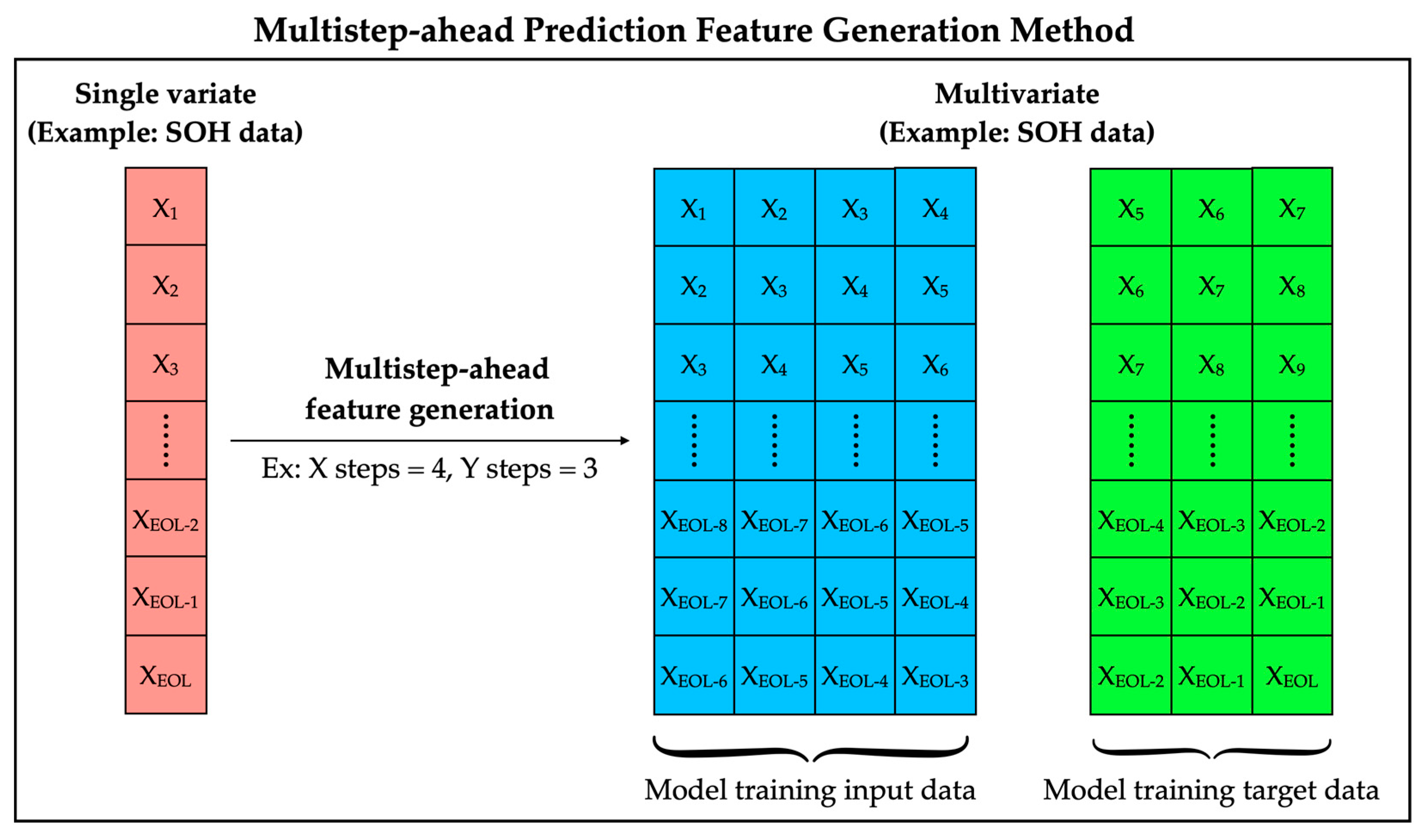After that, a multistep-ahead prediction feature generation method generates the training input and target data by choosing X steps and Y steps parameters and changing a single variate of SOH to multivariate. The multistep-ahead prediction feature method can achieve multiple step-ahead rolling future prediction by generating different X stamps and Y stamps training data, which represent the input data with X steps to predict Y steps ground truth data. Finally, the model hyperparameters tuning and prediction parameters of X steps and Y steps optimization are based on the Differential Evolution (DE) optimization algorithm. We only save the BiLSTM-AT model weights with lower loss than the last optimization iteration during the model optimization process. The DE optimization with a hybridized loss function combines three different loss functions defined based on our future capacity prediction problem. The detailed description of the hybridized loss function is shown in Section 3.3.

The target data simulate the online prediction process from the first cycle. The RUL prediction activated by the SOH of the target data reaches the SOH value of the starting point SOH_Tsp. We compute the knee point using the Bacon–Watts model to find a suitable fine-tuning training length for the target data. The point represents the early warning for accelerated SOH degradation. Finally, the training length defines the cycle from the knee point to SOH_Tsp. The BiLSTM-AT model weights and prediction parameters of X and Y steps are transferred from the source data to the target data. The BiLSTM-AT layer weights are froze for fine-tuning the model, which does not update in the fine-tuned model training. The only update layer is the output layer of the BiLSTM-AT model. In the end of the online prediction is the multistep-ahead rolling prediction for the RUL prediction. When the rolling prediction results reach 0.800, the rolling prediction stops and calculates the RUL prediction error and prediction interval by the Monte Carlo dropout approach.

3.1. Multistep-Ahead Prediction Feature Generation Method

To train more efficiently and achieve multistep-ahead rolling prediction for the future capacity prediction of the -AT model, we defined a multistep-ahead prediction feature generation method to generate the training input data and target data with different step parameters of X and Y steps to find a time series autoregressive relationship. The prediction parameters of this method are X steps and Y steps, representing the number of training input features and target ground truth steps. The operation of the technique is shown in Figure 2. This generation method for model input and target ground truth data helps find the autoregressive relationship within a single variate time series data for future rolling prediction. It improves the data-driven model to capture and learn seasonal, trend, and cyclical time series by training the BiLSTM-AT weights. Additionally, the generation method can achieve multistep-ahead rolling predictions based on the Y steps parameter, which controls the prediction steps for the future forecast.

3.2. Multistep-Ahead Rolling Prediction Method

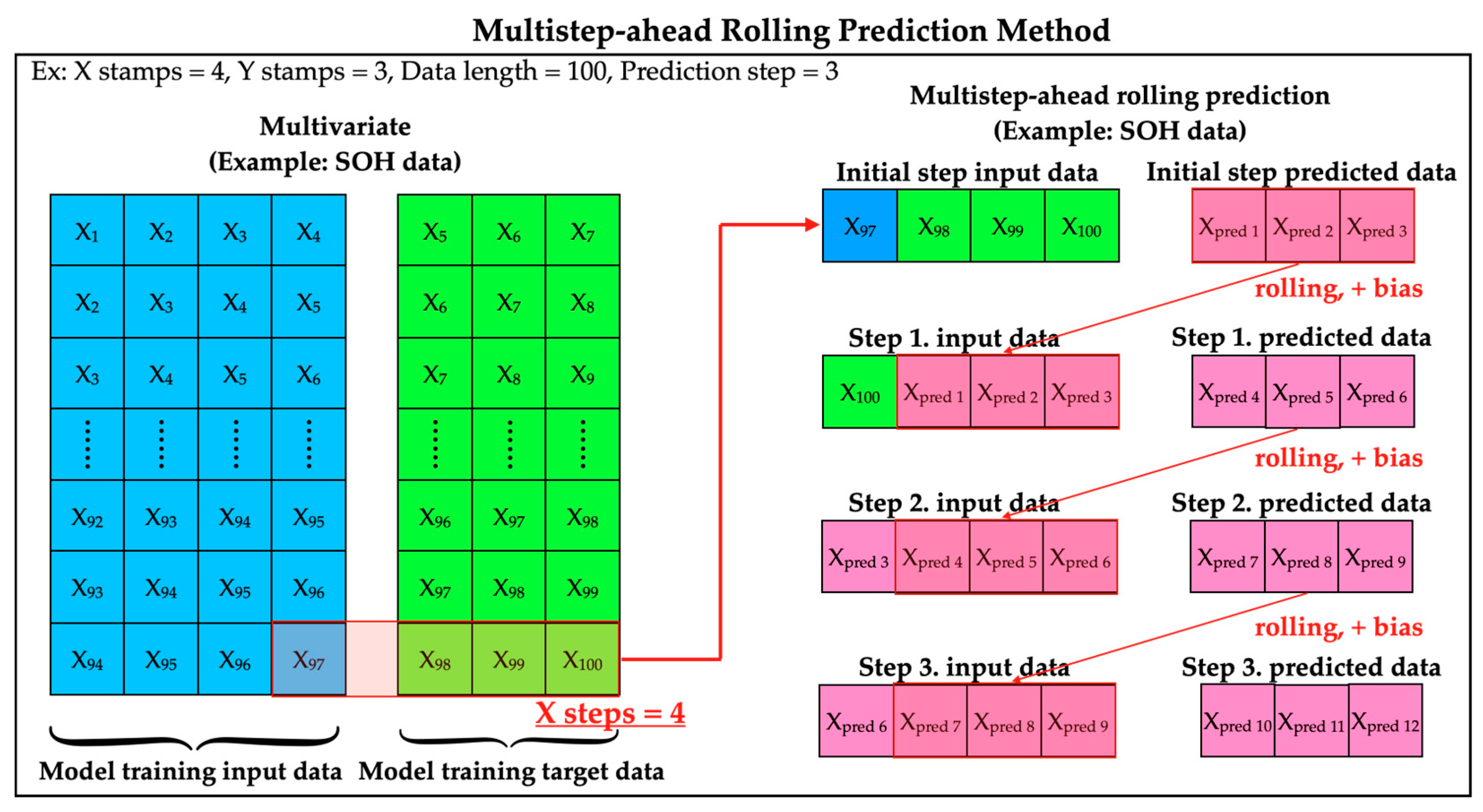
The steps of multistep-ahead rolling prediction are based on the Y steps parameter maintained in Section 3.1. We use a rolling prediction method to generate the next step of prediction based on the current step to achieve the future prediction. However, making an accurate future prediction is difficult because of the cumulative bias problem when generating more future steps. Figure 3 shows the operation of multistep-ahead rolling prediction. The cumulative bias problem is generated in each rolling prediction step, because selecting a stable Y steps parameter is an essential problem.

3.3. Deferential Evaluation Algorithm for Hyperparameter Optimization

Six hyperparameters deeply affect the multistep-ahead rolling prediction performance. Those hyperparameters exist side by side and play a part together in future prediction. We chose the DE algorithm as the optimization method to find the optimal hyperparameters automatically for BiLSTM-AT model training and prediction parameters because of its high speed and characteristics. The hyperparameters selected for optimization are X steps, Y steps, hidden size, batch size, dropout rate, and epoch. The hyperparameters bound for the DE algorithm searching are shown in

Table 1. Hyperparameters bound for DE algorithm.

Hyperparameter	Bounds	Data Type
X stamps	From 6 to 12	Integer
Y stamps	From 1 to 5	Integer
Hidden size	From 12 to 100	Integer
Batch size	From 8 to 128	Integer
Dropout rate	From 0.01 to 0.1	Float
Epoch	From 100 to 1000	Integer

. The most critical hyperparameters are X and Y steps because of their impact on the data-driven model capture of the time series relationship and the multistep-ahead rolling prediction bias cumulation problem. The predicted value will be used as the input for generating the next step of prediction. The Y stamps selected as one, three, and five represent the bias for each selection: one step of bias, three steps of bias, and five steps of bias generated, respectively. 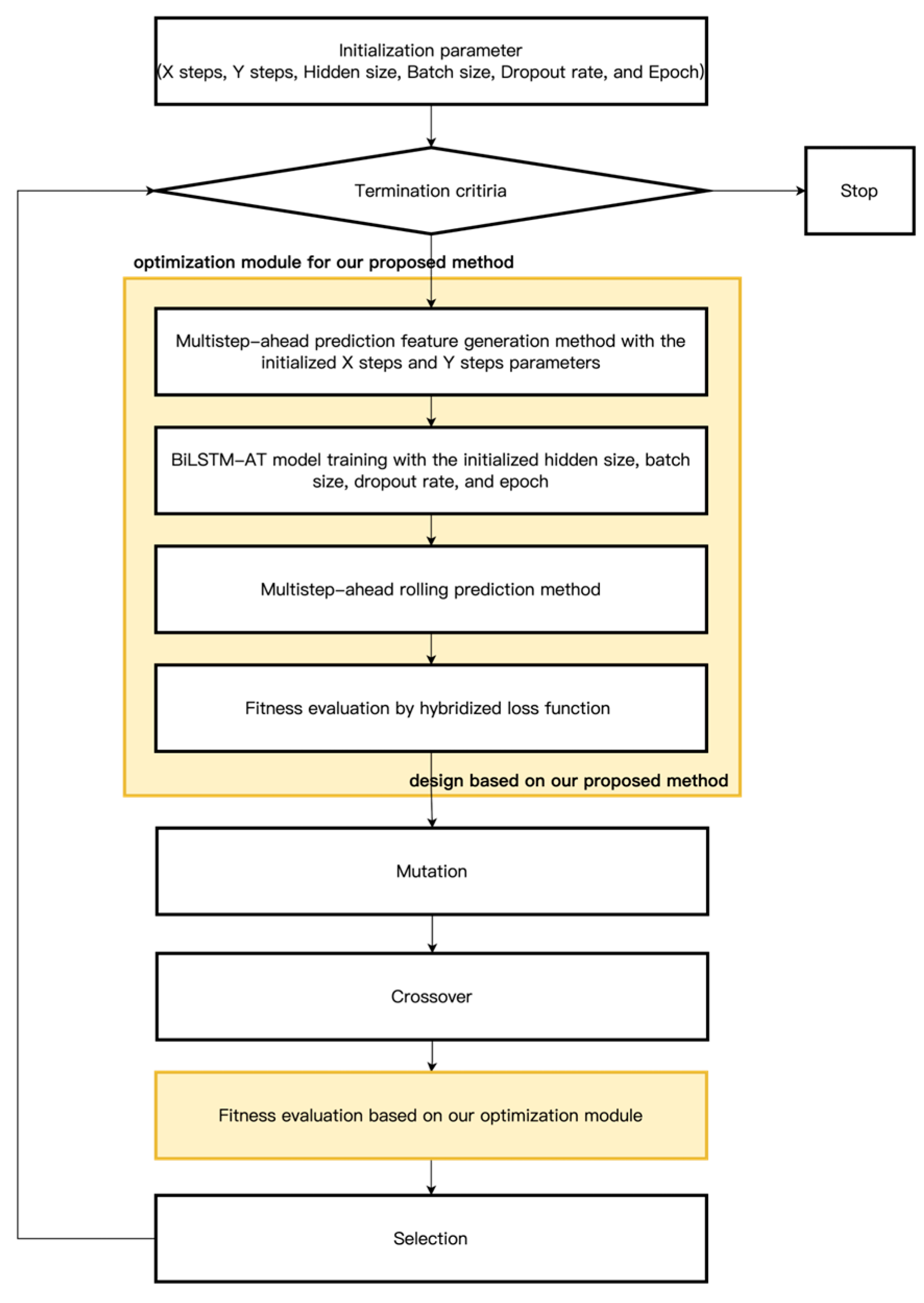Figure 4 shows the DE algorithm operation for our proposed method application.

At the beginning of the DE algorithm is the initialization of the parameters. The parameters are initialized based on the upper and lower bound and Uniform distribution as shown in Equation (3). X represents the initialized parameter, i is the number of populations, and j is the number of parameters. The min and max define the parameter bounds for the optimization search.

$$X_{i,j,0}=X_{\min }^j+\mathrm{U}\left(0,1\right)\times \left(X_{\max }^j–X_{\min }^j\right).$$

(3)

The optimization module design based on the proposed method consists of a multistep-ahead prediction feature generation method, BiLSTM-AT model training with the initialized parameters, a multistep-ahead rolling prediction method, and hybridized loss function for fitness evaluation. The performance of the hybridized loss function explains in Section 3.4. For the mutation a DE/best/1/bin strategy select to calculate the first-order difference between two of the vectors to the third in the following Equation (4).

$$V_{j,i,g+1}=X_{r1,g}+F(X_{r2,g}–X_{r3,g})$$

(4)

where V is defined as the donor vector, i represent the current population, g is the generation times, and r1, r2, and r3 are three samples randomly drawn from the population. However, the current population cannot be r1, r2, and r3. F is the mutation factor constant from [0, 1]. It is an essential parameter that controls the convergent speed and DE performance. In the crossover, a random variable generated from the uniform distribution with a CR parameter holds the trail vector U_{i, j, g+1} updated the current samples of the current population or not see Equations (5) and (6). Where j is the samples of current population.

$$U_{j,i,g+1}=\left\{\begin{array}{c}{V}_{j,i,g+1},\mathrm{if}\mathrm{random}\mathrm{number}\le \mathrm{CR},\\ X_{j,i,g+1},\mathrm{if}\mathrm{random}\mathrm{number}>\mathrm{CR}.\end{array}\right.$$

(5)

$$X_{i,g+1}\left\{\begin{array}{c}{U}_{i,g+1},\mathrm{if}f\left(U_{i,g+1}\right)\le f\left(X_{i,g}\right),\\ X_{i,g},\mathrm{otherwise},\end{array}\right.$$

(6)

where f represents the objective function to evaluate the parameter performance of the proposed module. In this paper, the objective function design is based on our proposed optimization module, the hybridized loss function, which is the objective function described in Section 3.4.

3.4. A Hybridized Loss Function for Optimization

However, a suitable loss function is an important problem for an optimization algorithm. Here, we define a hybridized loss function that consists of a Dynamic Time Warping (DTW) algorithm, the absolute error function, and the Mean Squared Error (MSE) in the following Equation (7). The DTW algorithm uses to compute the similarity between the predicted SOH and ground truth SOH and absolute loss function uses for calculating the difference between the length of predicted SOH and ground truth. Finally, MSE loss function compute the last point of the predicted SOH and ground truth SOH.

$$\begin{gathered} \mathrm{Hybridized}\mathrm{loss}\mathrm{function}=\mathrm{DTW}\left({\mathrm{SOH}}_{\mathrm{predicted}},{\mathrm{SOH}}_{\mathrm{ground}\mathrm{t}\mathrm{r}\mathrm{uth}}\right)+ \\ \left|\mathrm{length}\left({\mathrm{SOH}}_{\mathrm{predicted}}\right)-\mathrm{length}\left({\mathrm{SOH}}_{\mathrm{ground}\mathrm{truth}}\right)\right|+{\left|{{\mathrm{SOH}}_{\mathrm{predicted}}}_{T_{\mathrm{last}}}-{{\mathrm{SOH}}_{\mathrm{ground}\mathrm{truth}}}_{{\mathrm{T}}_{\mathrm{last}}}\right|}^2 \end{gathered}$$

(7)

We used multistep-ahead rolling prediction to evaluate the model performance for hyperparameter and prediction parameter optimization. There were three loss functions selected and combined. These three functions are essential and meaningful because of the designation for multiple step-ahead rolling predictions. Because of the length between the future prediction results of SOH by multistep-ahead rolling forecasts and the ground truth, the SOH may be different. According to this issue, the DTW algorithm is the best method to compute the similarity between two time series sequences. To increase the converging time of DE algorithm optimization, we added a loss function to calculate the length between predicted SOH and ground truth SOH. This loss function is resealable because of the RUL prediction indicated while considering the length from the SOH_Tsp to SOH_tEOL. Finally, the MSE of the last predicted SOH and ground truth SOH point was selected because the stopping rule of RUL prediction was the predicted SOH reaching SOH_tEOL and the ground truth SOH_tEOL being close to SOH_tEOL. 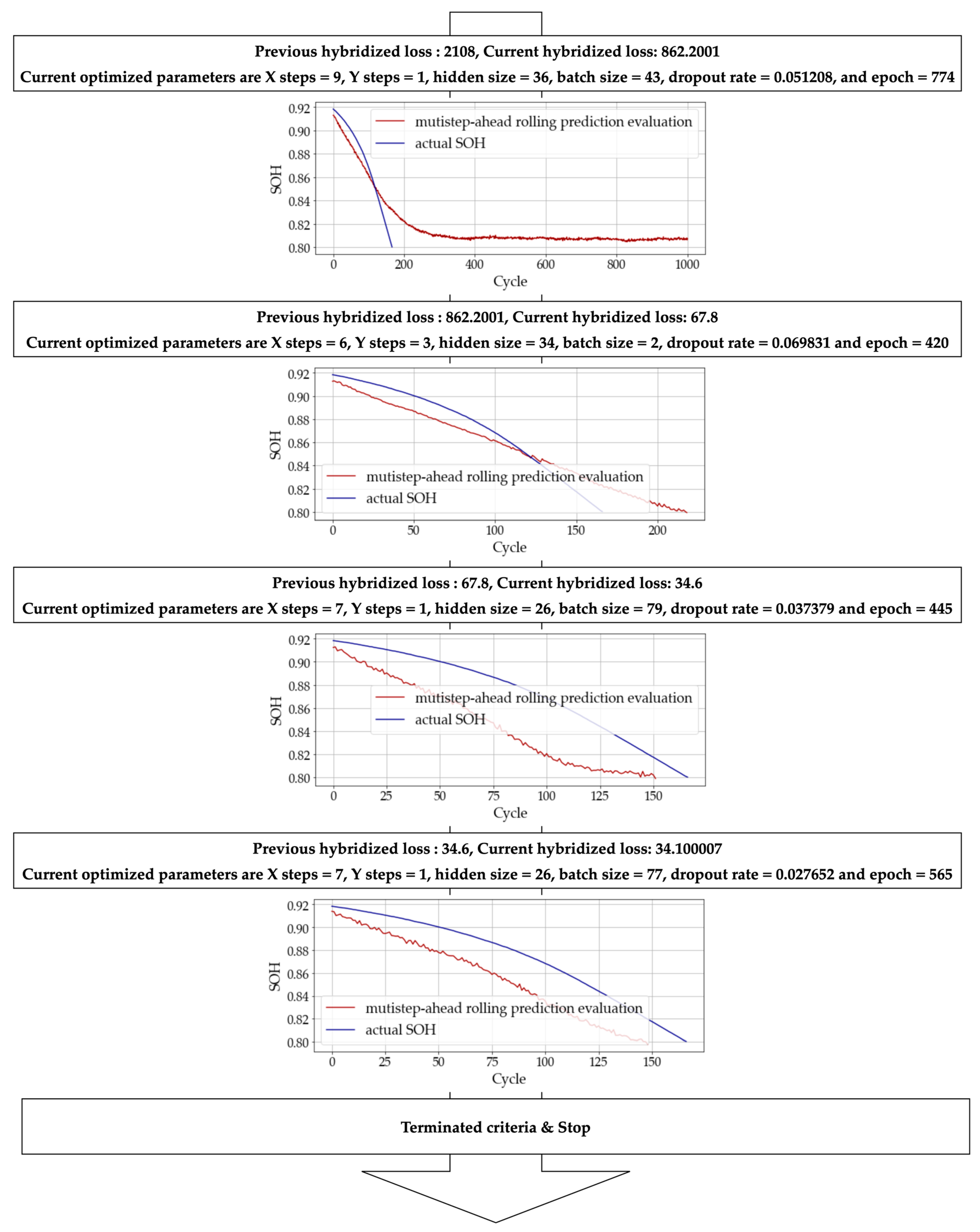Figure 5 shows the prediction and ground truth during DE algorithm optimization for finding the optimal hyperparameters.

The results obtained from Figure 6 indicate that the proposed method for multistep-ahead prediction is highly accurate, with predictions closely matching the actual target ground truth SOH sequence for each DE algorithm iteration. This is a strong indication that the three combined loss functions used in the model are appropriate and effective for optimizing the model’s hyperparameters. The accuracy of the multistep-ahead prediction is crucial for practical applications, where accurate predictions are necessary for effective battery management and maintenance. The fact that the proposed method achieves accurate predictions shows that it has the potential to be a valuable tool in the field of battery management, allowing for more efficient and effective battery maintenance and replacement strategies. The combination of the three loss functions, working together to optimize the model’s hyperparameters, is a key factor in the success of the proposed method, demonstrating the importance of careful parameter tuning in achieving accurate predictions in battery management systems.

3.5. Transfer Learning and Model Fine Tuning

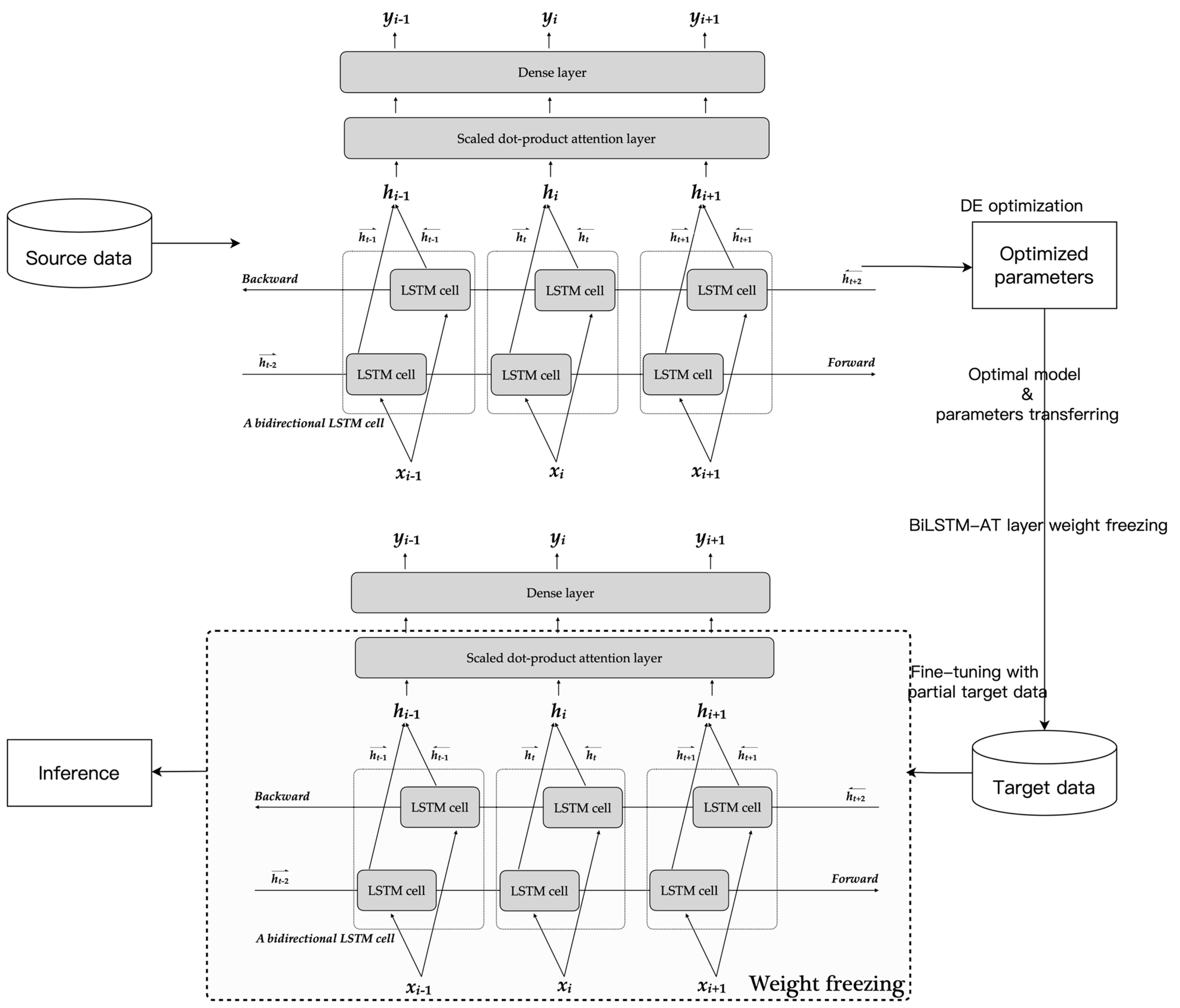
The proposed method for future capacity prediction in battery management systems involves the transfer of optimal BiLSTM-AT model weights and prediction parameters from source data to target data. The transfer process is accomplished by fine-tuning the output layer weights of the BiLSTM-AT model, as illustrated in Figure 6. This fine-tuning process improves the model’s adaptability to target data, as the source and target data may not necessarily belong to the same domain.

To ensure the effective fine-tuning of the BiLSTM-AT model, we carefully selected the hyperparameters, which include the learning rate and epoch. To avoid overfitting, a small learning rate of 0.01 was chosen, and a stopping rule was defined to halt the fine-tuning process when the BiLSTM-AT model fine-tuning loss does not reduce for ten consecutive epochs. This ensures that the fine-tuning process stops at an optimal point, and the output layer weights are updated accordingly, as discussed in Section 4 of the experiment results.

The proposed method is expected to be effective in predicting the future capacity of Li-ion batteries and can be applied in predictive maintenance to provide early warning of battery failure. The fine-tuning process enhances the model’s performance and reliability by ensuring that it is adapted to the target data. Furthermore, the transfer learning approach employed in the proposed method saves a significant amount of training time, making it suitable for online prediction. Overall, the proposed method demonstrates superior performance compared to other related models, making it a promising tool for battery management systems.

The BiLSTM-AT model is composed of two LSTM cells, which operate in opposite directions-one going forward and the other going backward. These cells are responsible for capturing the dependencies within their respective sequences. Each LSTM cell contains three gates, namely input, forget, and output gates, which regulate the flow of information in the memory cell. The input gate determines how much of the new input should be used to update the cell state, while the forget gate decides how much of the previous cell state should be retained. The output gate controls how much of the cell state is exposed to the output at each time step. The attention mechanism is also incorporated into the BiLSTM-AT model to improve its performance in learning from time series data by highlighting the significant features in the input sequence. The formulation of the forget gate f_t, input gate i_t, output gate o_t, and cell state c_t (∀t in domain) are shown in Equation (8).

f_t = sigmoid(W_fX_t + H_fh_t−1 + b_t),
i_t = sigmoid(W_iX_t + H_ih_t−1 + b_i) ⊗ tanh(W_cX_t + H_ch_t−1 + b_i),
o_t = sigmoid(W_oX_t + H_oh_t−1 + b_o) ⊗ c_t,
c_t = f_t ⊗ c_t−1 + i_t,

(8)

where W_f, W_i, W_o, and W_c are the forget, input, and cell state weights. X_t is the current input data, and H_f, H_i, and H_o represent the weights parameter of the hidden state in forget, input, and output gate, respectively. The parameter of h_t−1 is the previous hidden state, and b_t, b_i, b_o, and b_c are the bias in forget, input, output gate, and cell state. The forget gate controls the previous c_t−1 update or not by a sigmoid function’s output range from 0 to 1. The input gate uses a sigmoid function to update the cell state to decide the critical values, and the tanh function is used to normalize the previous hidden state and input data to range from –1 to 1. Finally, the sigmoid and tanh function output is computed via pointwise multiplication together to update the cell state. Last but not least is the output gate, which adds and updates the hidden state by calculating the output of the sigmoid function with the previous hidden state and input data and pointwise multiplication with the cell state.

To improve the model performance, a bidirectional hidden learning method is selected to capture the forward and backward information X_t form hidden state transmission process as shown in Equation (9). The forward hidden state represents the ${\stackrel{⃑}{h}}_t$ between the start recurrent cell and the end recurrent cell; it controls the updating of the weight the LSTM cell at the next recurrent cell. The backward hidden state represents the ${\stackrel{⃐}{h}}_t$ from the end recurrent cell to the first recurrent cell. It transmits the information from the back to the first cell and controls the weight updating of the LSTM cell. Finally, the output y_t combines the forward and backward results from the LSTM cell.

$$\begin{gathered} {\stackrel{⃑}{h}}_t={\mathit{LSTM}}_{\mathit{cell}}\left(X_t,{\stackrel{⃑}{h}}_{t-1}\right), \\ {\stackrel{⃐}{h}}_t={\mathit{LSTM}}_{\mathit{cell}}\left(X_t,{\stackrel{⃐}{h}}_{t+1}\right), \\ {y}_t=W_{{\stackrel{⃑}{h}}_t}{\stackrel{⃑}{h}}_t+W_{{\stackrel{⃐}{h}}_t}{\stackrel{⃐}{h}}_t+b_{y_t}. \end{gathered}$$

(9)

The main contribution of our paper is the introduction of a new attention mechanism, called scale dot-product attention, which we combine with the BiLSTM-AT model to enhance its ability to learn from time series data. This attention mechanism helps the model to automatically learn the complex relationships between the model output and hidden state, which is important for accurately predicting future battery capacity. Overall, our proposed attention mechanism enhances the performance of the BiLSTM-AT model, enabling it to better learn the relationships between the input and output variables in time series data. This has important applications for battery management systems, where accurate predictions of future capacity are crucial for maximizing battery lifespan and minimizing downtime.

The input components of the scale dot-product attention consist of q of the query vector, k of the key vector, and v of the value vector; see Equation (10), where $\sqrt{d_k}$ is the scale factor calculated from the hidden neuron size, and the output of the SoftMax activation function is a probability value representing the importance of the weight from zero to one. Finally, the value vector multiplies the output of the SoftMax function and gives it the weighting.

$${\mathit{Attention}}_{\mathit{scale}-\mathit{dot}}\left(\mathit{q},\mathit{k},\mathit{v}\right)=\mathrm{Soft}\max (\frac{\mathit{q}{\mathit{k}}^{\mathit{T}}}{\sqrt{d_k}})\mathit{v}.$$

(10)

4. Analysis Results and Discussion

For model robustness and operability experiments, the proposed method was evaluated using three groups of nine cells, all of which were high-power LFP/graphite A123 APR18650M1A cells [19]. The batteries were tested under different fast charge and discharge conditions in the same environmental chamber at 30 °C. The normal capacity was 1.1 Ah and the voltage was 3.3 V. In our experiments, each group selected one battery as source data and the remaining two as target data. The BiLSTM-AT model trained only once with the source data and optimized each battery batch’s hyperparameters and prediction parameters. The training length for model training was defined from the cycle of knee-onset to the SOH_tEOL. For online prediction, the BiLSTM-AT model weights transferred and fine-tuned the output layer with partial target data representing the gap from the knee point to SOHT_sp. Our experiments changed different SOH_Tsp to test the proposed method performance, which was 0.888, 0.875, and 0.860. The first experiment was Battery#1, followed by Battery#2 and Battery#3 tested in the same charging policy. 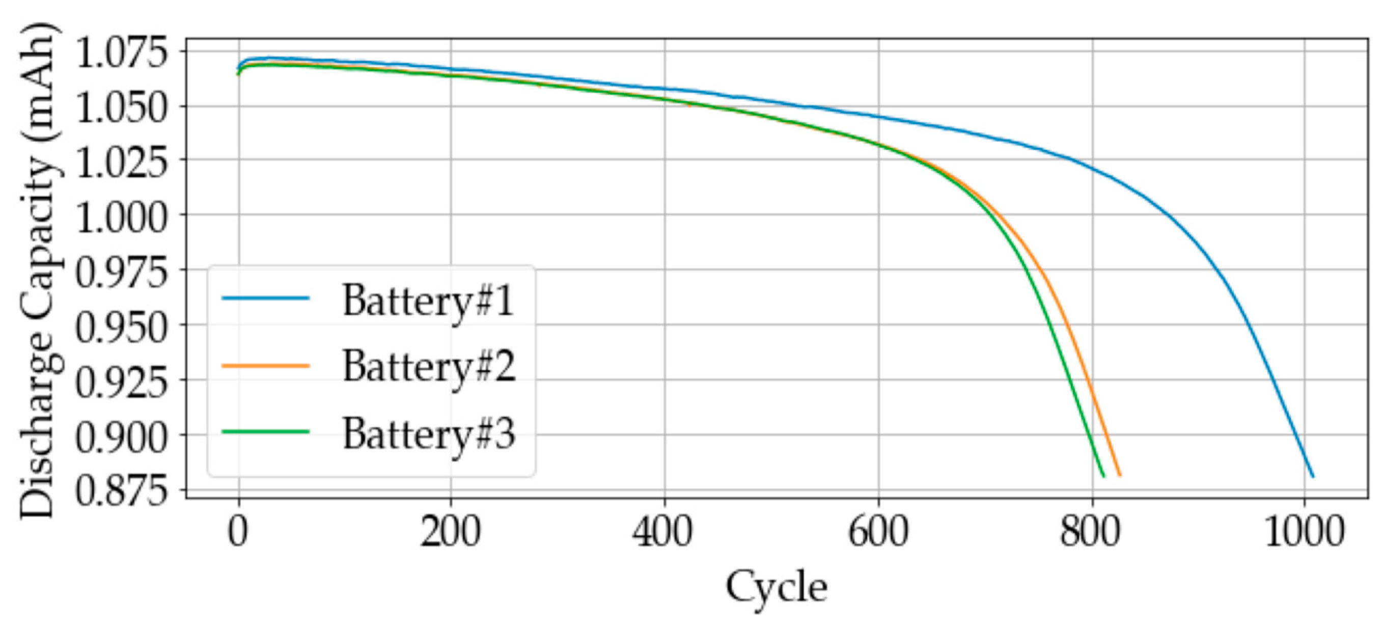The SOH_EOL was defined at 0.800 because the battery was dead in the SOH, reaching 0.800 on Battery#1 (see the discharge capacity curve of these three batteries in Figure 7). We selected Battery#1 as the source data. Battery #2 and Battery#3 were chosen to be the target data to test the proposed method’s performance.

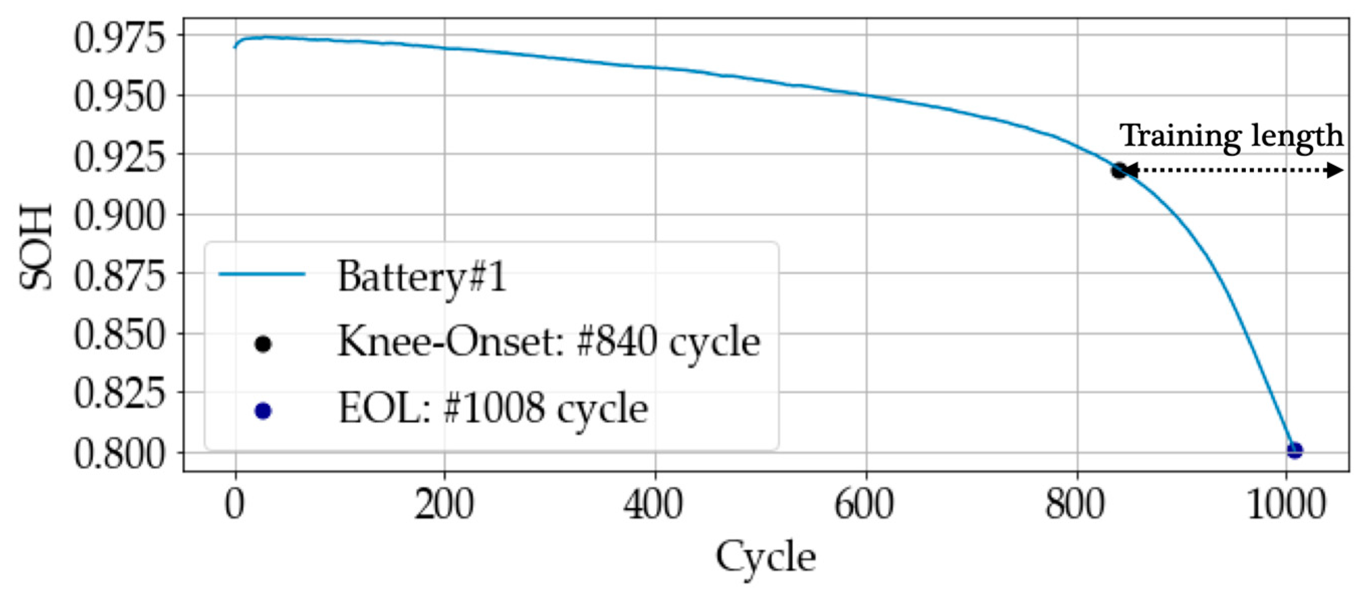
Figure 7 shows that the battery in the same charging policy has similar degradation discharge capacity patterns. Because of the pattern reproducibility, the proposed method can keep transferring and fine-tuning different source data with the same charging policy. The training length of target data Battery#1 is defined from the cycle of knee-onset to SOH_tEOL, as shown in Figure 8. The knee-onset was calculated using the double Bacon–Watts model. The DE algorithm optimized the whole model training process for the model training, which contains a multistep-ahead prediction feature generation method and BiLSTM-AT model training. We optimized the prediction parameters and BiLSTM-AT hyperparameters by setting the reasonable parameter bounds shown in Table 1. The DE algorithm optimizes the parameters based on the multistep-ahead rolling prediction and computes the hybridized loss to find the optimal parameters that perform best. The optimal hyperparameters and prediction parameters are X steps = 5, Y step = 1, hidden size = 71, batch size = 64, dropout rate = 0.0001, and epoch = 850 for source data Battery#1. Figure 9 and Figure 10 show the DE optimization loss in each iteration and the last iteration result of multistep-ahead rolling prediction results.

When the SOH value reached SOH_Tsp, we computed the knee-onset point to define the training length for the model fine-tuning by partial target data. The target data of Battery#2 and Battery#3 were simulated from the first cycle to the end. The learning rate and epoch were set as 0.01 and 10,000, respectively, with the early stopping role to avoid the overfitting problem for model fine-tuning, as we explain in Section 3.5. From Figure 11, the stopping rule for three different SOH_Tsp values of Battery#2 and Battery#3 was 35, 26, and 31 and 18, 30, and 26, respectively.

Finally, the multistep-ahead rolling prediction dealt with future capacity prediction for target data. When the predicted SOH value reached SOH_EOL, the multistep rolling prediction was stopped and the performance of RUL prediction using the relative error and absolute error was calculated. The performance metric computation for Battery#2 and Battery#3 online prediction experiments of SOH_Tsp, equaling 0.888, 0.875, and 0.860, is shown in

Table 2. The multistep-ahead rolling prediction RUL performance for Battery#2.

Battery	Starting Point	Actual RUL	Predicted RUL	AE	RE (%)
#2	750 (SOHTsp = 0.888)	77	54	8	17.39
#2	767 (SOHTsp = 0.875)	60	54	6	10.00
#2	781 (SOHTsp = 0.860)	46	50	4	8.70

and

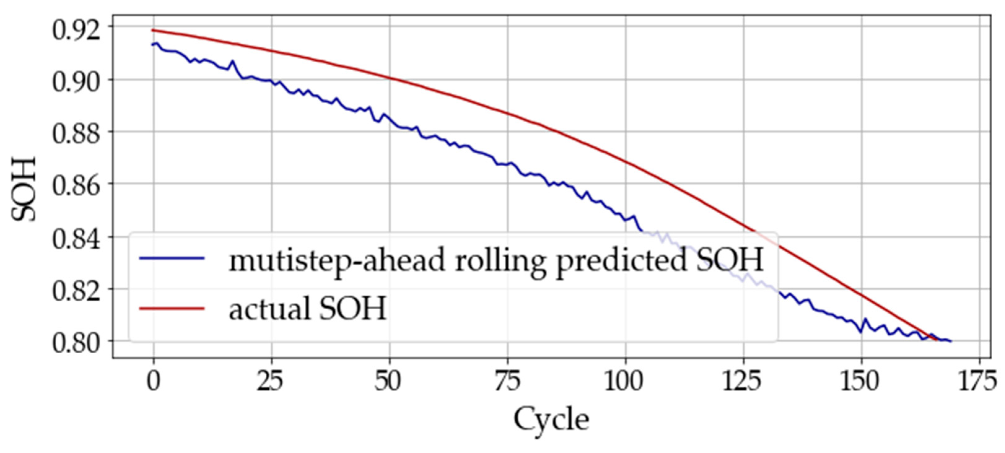
Table 3. The multistep-ahead rolling prediction RUL performance for Battery#3.

Battery	Starting Point	Actual RUL	Predicted RUL	AE	RE (%)
#3	738 (SOHTsp = 0.888)	74	66	8	10.81
#3	751 (SOHTsp = 0.875)	61	56	5	8.20
#3	765 (SOHTsp = 0.875)	47	44	3	6.38

. The multistep-ahead rolling prediction performance results of source data Battery#2 and Battery#3 are shown in Figure 12. Table 2 shows that the AE and RE (%) for the source data Battery#2 in three scenarios are 8, 6, and 4 and 17.39, 10.00, and 8.70, respectively. The RUL performance of source data Battery#3 in three scenarios is 8, 5, and 3 and 10.81, 8.20, and 6.38, respectively.

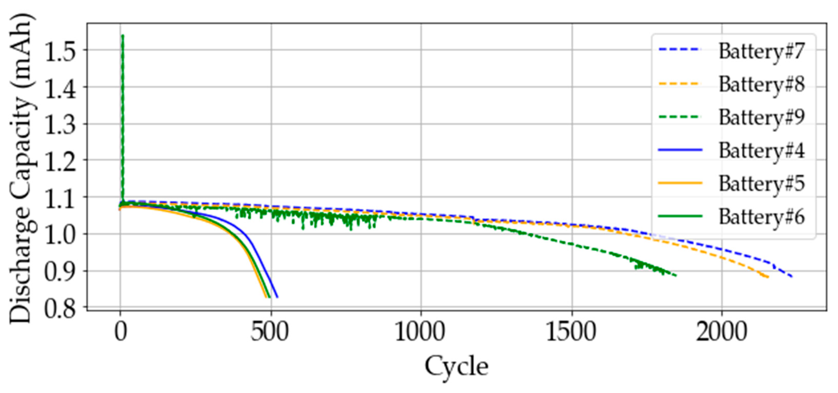
To test the performance and robustness of the proposed fine-tuning model based on the transfer learning method, we added two batches of batteries with different charging policies. The additional batches were used in the proposed method to experiment. The additional batches containing Batteries #4, #5, and #6 had the same charging policy to experiment with the proposed method. Other batches consisting of Battery#7, Battery#8, and Battery#9 had the same charging policy. Figure 13 shows the additional batches’ experiment discharge capacity. The same lifestyle represents the battery in the same charging policy. From the discharge capacity curve, we can understand the battery in different charging policies with different degradation curves and the battery in the same charging policy with a similar degradation curve. The proposed method can solve the future capacity prediction of Li-ion batteries in the same charging policy and accurately predict the future degradation curve.

The RUL performances in multistep-ahead rolling prediction for the first batch containing Battery#4, Battery#5, and Battery#6 are shown below in

Table 4. The multistep-ahead rolling prediction RUL performance for Battery#5.

Battery	Starting Point	Actual RUL	Predicted RUL	AE	RE (%)
#5	397 (SOHTsp = 0.888)	90	78	12	13.33
#5	410 (SOHTsp = 0.875)	77	68	9	11.69
#5	424 (SOHTsp = 0.860)	63	57	6	9.52

and

Table 5. The multistep-ahead rolling prediction RUL performance for Battery#6.

Battery	Starting Point	Actual RUL	Predicted RUL	AE	RE (%)
#6	404 (SOHTsp = 0.888)	94	80	14	14.89
#6	418 (SOHTsp = 0.875)	80	70	10	12.50
#6	432 (SOHTsp = 0.860)	66	71	5	7.58

. Battery#4 was selected as the source data in this batch. We transferred the BiLSTM-AT model weights, model hyperparameters, and prediction parameters to the target data: Battery#5 and Battery#6. Three different SOH_Tsp scenarios were used to test the proposed method with the multistep-ahead rolling prediction. From Table 4 and Table 5, the three various SOH_Tsp scenario experiments show the future capacity prediction by the proposed fine-tuning-model-based transfer learning method outperformed the others in terms of robustness and accuracy. The AE and RE (%) for the source data Battery#5 in three scenarios were 12, 9, and 6 and 13.33, 11.69, and 9.52, respectively. The RUL performance of source data Battery#6 in three scenarios was 14, 10, and 5 and 14.89, 12.50, and 7.57, respectively. The optimal hyperparameters and prediction parameters were X steps = 14, Y step = 1, hidden size = 82, batch size = 113, dropout rate = 0.0001, and epoch = 509 for transferring to the target data experiment.

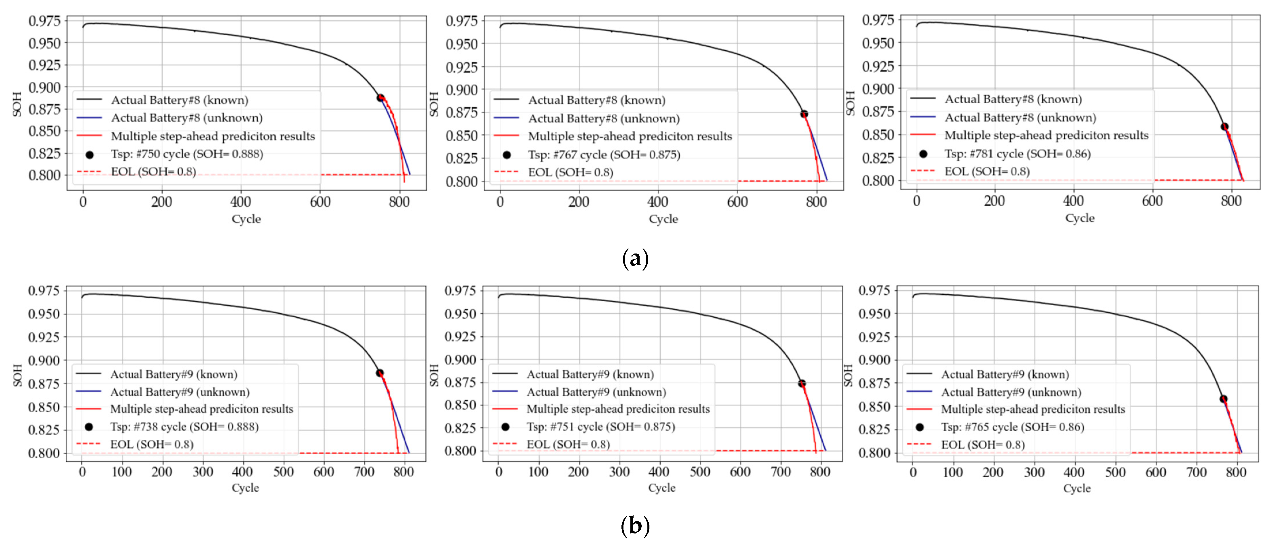
The final batch for the RUL performance experiment contained Battery#7, Battery#8, and Battery#9; the source data were selected to be Battery#7; and the target data were Battery#8 and Battery#9. For the three different SOH_Tsp scenarios for performing the proposed method, see

Table 6. The multistep-ahead rolling prediction RUL performance for Battery#82.

Battery	Starting Point	Actual RUL	Predicted RUL	AE	RE (%)
#8	1805 (SOHTsp = 0.888)	353	372	19	5.38
#8	1878 (SOHTsp = 0.875)	280	288	8	2.86
#8	1952 (SOHTsp = 0.860)	206	210	4	1.94

and

Table 7. The multistep-ahead rolling prediction RUL performance for Battery#9.

Battery	Starting Point	Actual RUL	Predicted RUL	AE	RE (%)
#9	1464 (SOHTsp = 0.888)	386	368	18	4.66
#9	1533 (SOHTsp = 0.875)	317	306	11	3.47
#9	1632 (SOHTsp = 0.860)	218	223	5	2.29

. The prediction length in the final batch experiment was longer than in the other experiments. This means the steps of the rolling prediction step were more than the other experiments, and the prediction bias was as significant as the increase in the prediction steps. From Table 6 and Table 7, even the rolling prediction steps were more extended than the other experiments by approximately three times. The RUL performance shows the proposed method is helpful and reliable in a long-prediction-length experiment. The multistep-ahead rolling prediction results in three different scenarios of RE for Battery#8 were 5.38, 2.86 and 1.94 when the actual RUL was 372, 288, and 210, respectively. The experiment results of RE for Battery#9 were 4.66, 3.47, and 2.29 when the actual RUL was 18, 11, and 5, respectively. The model hyperparameters and prediction parameters for the final batch were X steps = 10, Y step = 6, hidden size = 94, batch size = 10, dropout rate = 0.0001, and epoch = 564 for transferring to the target data experiment.

After analyzing and discussing our results, we found that our proposed method for predicting future battery capacity using a fine-tuning model with transfer learning outperforms other methods and demonstrates strong reliability. Our method utilizes data from a single battery as the source data, and then transfers the optimized model weights, hyperparameters, and prediction parameters to achieve accurate future results for RUL prediction, even over long prediction horizons. We found that our method is able to achieve high accuracy across a range of prediction steps, and that it outperforms other methods that do not incorporate transfer learning or fine-tuning. By fine-tuning our model using partial target data, we are able to achieve more accurate predictions, even when working with limited data. Additionally, our approach is flexible and can be applied to a wide range of battery types and applications, making it a valuable tool for battery management and predictive maintenance. Overall, our experimental results suggest that our proposed method is a reliable and effective way to predict the future capacity of Li-ion batteries.

5. Conclusions

The major contribution of this paper describes the use of transfer learning to address the issue of data scarcity by fine-tuning a pre-trained model on a target dataset. The process involves adjusting the pre-trained model’s parameters to improve its performance on the specific task and dataset. We also discuss the use of sliding window methodology to improve the accuracy of predicting future capacity for Li-ion batteries. A hybrid loss function is proposed to evaluate the performance of the model during the optimization of hyperparameters and prediction parameters, which combines multiple criteria for assessing the model’s performance into a single objective function that can be optimized using gradient-based methods.

In summary, the future capacity prediction of Li-ion batteries is an important area of research in battery management systems. Our proposed method uses a deep learning model with transfer learning, divided into offline training and online prediction stages. By transferring the model weights and prediction parameters from offline training to online prediction, and fine-tuning them with partial target data, our method achieves accurate results with a relative error ranging from 1.94% to 9.52% for six target batteries under SOH_Tsp = 0.860 in online prediction. This approach is effective in predicting future battery capacity and can be applied for predictive maintenance, providing early warnings of battery failure. Compared to other related models, our transfer learning approach offers better results and saves considerable training time, making it suitable for online prediction. Overall, our proposed online prediction method has practical applications for battery maintenance and replacement strategies.

In the future, we plan to expand our proposed model to predict the capacity of multiple target batteries using data from multiple source batteries. This will involve developing a more complex model that can handle a larger and more diverse set of data inputs, potentially incorporating additional features or sensor data to improve the accuracy of our predictions. Additionally, we will need to carefully evaluate the performance of our model on these more complex prediction tasks, potentially using metrics such as mean absolute error or root mean squared error to assess the quality of our predictions. Ultimately, the goal of this research will be to create a powerful and flexible battery management system that can accurately predict the behavior of multiple batteries in a variety of real-world scenarios.