Model-Based State-of-Charge and State-of-Health Estimation Algorithms Utilizing a New Free Lithium-Ion Battery Cell Dataset for Benchmarking Purposes

Abstract

State estimation for lithium-ion battery cells has been the topic of many publications concerning the different states of a battery cell. They often focus on a battery cell’s state of charge (SOC) or state of health (SOH). Therefore, this paper introduces, on the one hand, a new lithium-ion battery dataset with dynamic validation data over degradation and, on the other hand, a model-based SOC and SOH estimation based on this dataset as a reference. An unscented Kalman-filter-based approach was used for SOC estimation and extended with a holistic ageing model to handle the SOH estimation. The paper describes the dataset, the models, the parameterisation, the implementation of the state estimations, and their validation using parts of the dataset, resulting in SOC and SOH estimations over the entire battery life. The results show that the dataset can be used to extract parameters, design models based on it, and validate it with dynamically degraded battery cells. The work provides an approach and dataset for better performance evaluations, applicability, and reliability investigations.

1. Introduction

For lithium-ion batteries in applications, it must be ensured that they are operated in a safe operating area (SOA). The SOA includes boundaries for the voltage, the temperature, and the current [1,2]. To support this, different battery states must be tracked during operation. In addition, the battery management system (BMS) should guarantee a reliable and efficient operation to ensure a safe operation. Therefore, the BMS’s tasks include collecting measurements of voltages, temperatures, and the system current to ensure operation in the SOA and the estimation of the battery states that support the task for a safe and efficient operation [3]. The typical states the BMS estimates for lithium-ion batteries include the state of charge (SOC), the state of function (SOF), the state of health (SOH), and the remaining useful life (RUL). Additional states are sometimes mentioned in the literature, such as the state of balance or the state of temperature. This paper considers two of these battery cell states because of their importance in a BMS. The state of charge (SOC) generally describes the charge available in the battery cell compared to a fully charged cell. Therefore, the SOC describes how long a battery cell may last with this charge and, thus, reflects in an electric vehicle the remaining range, similar to a fuel gauge in an internal combustion engine vehicle. Electrochemically, it describes the average lithium concentration of intercalated ions in the negative electrode. This is why the SOC cannot be directly measured in an application. The cell voltage includes the SOC to some extent, mainly the relation of the OCV and SOC, but the surface concentration of lithium ions influences it, in contrast to the SOC [1,2,3,4,5,6]. Since the SOC is essential for improving efficiency and influences battery cell ageing, it has to be estimated. A further hindrance is that it highly depends on the actual capacity of the battery cell, which is affected by the temperature, the state of ageing, and the current rate [1]. In addition to the general importance of the SOC, it is the foundation of other states. Its mathematical description is as follows.

$$\mathrm{SOC}=\frac{Q_{remain}}{C_{est}},$$

(1)

where $Q_{remain}$ describes the concentration of the intercalated lithium ions in the structure of the negative electrode, and $C_{Est}$ is the current maximum capacity (estimated or measured) based on the temperature and the ageing state.

The SOH describes the degradation of the battery cell. It describes the battery cell as having a 100% SOH when it is considered new. In most cases, the parameters used to describe the SOH are the capacity and the battery cell’s internal resistance (IR). The initial quantities of the capacity and IR can be either the nominal values gathered from the datasheet or the measured parameters during the first check-up. When using the nominal capacities, the SOH can be over 100% because of the production tolerances of the single battery cells. A classic definition of the SOH is based on the ratio of the estimated and the nominal or initial capacity

$${\mathrm{SOH}}_{\mathrm{C}}=\frac{C_{est}}{{\mathrm{C}}_{\mathrm{nom}}}.$$

(2)

This definition is specifically beneficial when the application is mainly interested in the energy capability of the battery cell. However, it could be extended with an SOH that is based on the battery cell’s internal resistance, defined by

$${\mathrm{SOH}}_{\mathrm{R}}=\left|\frac{R_{est}-{\mathrm{R}}_{\mathrm{EOL}}}{{\mathrm{R}}_{\mathrm{nom}}-{\mathrm{R}}_{\mathrm{EOL}}}\right|.$$

(3)

Depending on the scaling and combination of the definitions, the SOH describing the end of life could either be 80% or 0%. In this paper, it is 80%. This work aims to show a new, freely available dataset and how to use the data to implement an SOC and SOH estimation validated on the dynamic ageing dataset. It introduces and describes the measurements conducted and the development steps of a state estimation approach for SOC and is used in multiple applications based on the measurements. The parameterisation of the model used for the model-based approach for the SOC and SOH estimation is described and will be validated on dynamically aged battery cell data. Therefore, the paper sums up the approach for developing state estimation algorithms from the absolute beginning of the measurements to the modelling, algorithms, and validation at the end. It delivers the possibility to benchmark other state estimation algorithms in comparison to a common approach and allows for showing the advantages or disadvantages of developed approaches. Furthermore, the dataset could be used to develop new algorithms. Compared to other datasets found in the literature, the dataset includes the dynamic cyclic degradation of cells with changing stress factors. The paper of dos Reis et al. [7] includes a review of numerous datasets. Based on that paper, it can be concluded that the datasets available for cyclic ageing include only constant current charging and discharging. The datasets with driving cycles include only data with driving cycles for single cells [8,9], for packs [10], or for multiple cells under the same conditions [11]. The datasets do not include reference data and dynamical data, and if they include dynamical data, the stress factors stay the same for every iteration of the driving schedule. In contrast, the proposed dataset includes reference data with constant-current-cycled cells and dynamical data where the schedule starts repeating every 10 full-cycle equivalents.

A literature review of the different SOC and SOH algorithms shows different categories of algorithms. The categories derived are direct measurements, model-based approaches, data-driven approaches, and hybrids of two or more of these categories.

1.1. Direct Measurements for SOC and SOH Estimation

Direct measurement approaches in battery cell state estimation describe measurements that can be directly used to estimate a state. These could be specific parameters, just the voltage, temperature, or current at specified points in time, depending on the state to be estimated.

One typical measurement is the measurement of the OCV to use the relation of the SOC and the OCV. The relation is measured before application of the battery cell and used during its runtime to estimate the SOC [12]. The OCV can be measured after hours without a current, therefore, in an application, the assumption that the overpotential, either after a short resting phase or during a low-current section, is nearly equal to the true OCV, is applied, which is similar to the assumption for performing the short-term incremental OCV measurement and the low-current measurement, because in many cases there are no long resting phases. Often there are still small currents to supply the control units. This kind of SOC estimation is often used for calibration, to augment other algorithms, or under laboratory conditions [3]. An analysis based on the relation of the OCV and the SOC that slightly changes with degradation is used to estimate the SOH. This analysis is called the incremental capacity analysis (ICA) and describes the differentiation of the charge over the voltage, leading to peaks in the region of phase changes. The ICA is calculated from current measurements at constant currents for a full or a partial discharge/charge cycle. The battery cell’s SOH can be estimated by tracking the position, amplitude, and enveloped area [12,13]. Of course, the change in these peaks has to be investigated before the application to know which change belongs to which SOH. However, still, these measurements are only applicable in some applications.

There is the well-known coulomb counting method. The coulomb counting approach integrates the charged or discharged charge over time. That integrated value is divided by the current capacity to estimate the SOC. In this case, the starting point, the starting SOC, of the coulomb counting approach has to be known. The coulomb counting method depends on the capacity, therefore, on the SOH, and is influenced by the temperature and the current rate. This method is prone to measurement errors since they are accumulated over time [3,12]. Due to this disadvantage, it is often combined with the OCV measurement, where it is possible to recalibrate the counter. Based on the coulomb counter, a cycle counter can be established that counts the equivalent full cycles during usage. Therefore, it is extended such that it counts the charge in the charge direction or the absolute value of the current in both the charging and discharging directions and is divided by either the capacity or twice the capacity. To be able to use this information correctly, many measurements have to be taken to obtain the relation between the number of equivalent full cycles and the SOH, because the trajectory of the degradation depends on stress factors such as the current rate, the temperature, the $\Delta$DOD, and the mean voltage. The measurement of impedance or internal cell resistance is another method to estimate a state—especially the SOH’s correlation with the increase in the internal cell resistance. Different methods are used to measure the internal resistance. Sometimes people try to identify the internal resistance at current changes during the application and filter the results afterwards. However, this approach is often not measuring the actual internal resistance because the sample rate of the current and voltage measurement is too slow to isolate the internal resistance. So, what is measured is a combination of the internal resistance and the impedance of the active electrochemical processes. More common is applying a current pulse to identify the internal resistance [13,14]. Similarly, here, the measured resistance might not be the internal resistance, but it is a part of it. An electrochemical impedance spectroscopy (EIS) measurement with a single frequency is possible to measure the true internal resistance. More frequencies are applied to gain more information using, for example, a multi-sine approach or just different frequencies to a typical EIS measurement [3,13]. Furthermore, typically EIS is used in applications to obtain more information on the battery cell’s impedance. Different electrochemical mechanisms can be analysed without opening the cell by investigating the EIS. Therefore, it is very interesting to use EIS, since it is a tool that could make a good diagnostic of ageing processes possible [3,13,14]. The application of an EIS measurement is very complex because it is susceptible to changes in the measured system, which can be changes in the connection, temperature changes, and other disturbing influences. Another measurement technique that might be used is based on the Joule effect. This approach analyses the generated heat and the rise in the temperature of the battery cell to identify the internal resistance. However, a calorimeter is needed to track temperature change and heat generation [13,14]. Other measurement equipment might be used as well [13]. Of course, using a calorimeter as an online measurement tool is unsuitable.

1.2. Model-Based SOC and SOH Estimation

In general, model-based state estimation approaches depend on the model. It could be that the approach only uses a model or combines an algorithm such as a filter or observer with a model. Using models directly to estimate the battery cell state is primarily not used for SOC estimation. Suppose coulomb counting or the OCV relation to the SOC is considered model-based. Then, they are the only models for model-based SOC estimation. It is another case for SOH or RUL estimation. The basic models used for direct estimation are semi-empirical, empirical, and electrochemical ageing models used to estimate the SOH. Empirical and semi-empirical models are developed based on ageing measurements considering different stress factors. The model is fitted to the change in a parameter over time or full-cycle equivalents, i.e., the internal resistance or the capacity, and is used to calculate the current SOH or RUL considering the cycles or the time at a specific stress factor. A weighted coulomb-counter-based cycle counter can be used to track the influence of the stress factors. The same approach can be used if the empirical model is replaced with the degradation data saved in a characteristic map [12,13,15]. By using a more sophisticated model such as an electrochemical pseudo-two-dimensional model and using different ageing improvements, the extrapolation ability and, therefore, the prediction ability is improved for unseen data. In addition, the model can diagnose the ageing process. However, due to their complexity and the involvement of many parameters and multiple partial differential equations, they are unsuitable for online usage. Therefore, research has focused on simplifications and parameterisation [12,13]. Every other model-based state estimation approach includes a filter or observer. Filters and observers share that they use the same general framework. They both rely on the model-based prediction (time update) of the battery cell state and use the measurement to adjust the prediction (measurement update) to the current behaviour of the battery cell. Filters that are often used belong to the Kalman filter family, namely, the extended Kalman filter or sigma-point Kalman filter, of which the unscented Kalman filter is a member. They use the general approach of making model-based predictions and updating the prediction by measurement using the so-called Kalman gain. The different modifications of the Kalman filter try to linearise the system around the current working point using the derivative or an approximation. Known observers include the Luenberger and the sliding mode observer.

1.3. Data-Driven SOC and SOH Estimation

The data-driven approaches contain machine learning approaches that describe a group of algorithms capable of inferring a battery’s behaviour from raw data to build a model that can predict the output or a state depending on the data without directly programming it for this specific behaviour. The methods used for state estimation can be categorised into methods that directly predict the output based on data and the methods that iteratively predict the output, where the output could be a state, parameters, or the voltage of the battery cell. Whether the prediction structure is direct or iterative depends on the task and algorithm. An algorithm that makes point predictions can have a direct structure, whereas an algorithm that predicts sequences or simulates something will have an iterative structure. Depending on the output, they can be further distinguished into algorithms that produce outputs with a measure of certainty/probability or not, probabilistic or non-probabilistic methods. Machine learning approaches include neural networks, autoregressive-moving average models, and support vector machines [12,16].

1.4. Hybrid Estimation

Instead of estimating a single state, a joint or dual estimation can be applied. Joint estimation includes the estimation of the SOC and the SOH with one extended algorithm. In contrast, dual estimation is the estimation of the SOC and SOH using two algorithms working together. In joint estimation, the connection of the states is directly part of the estimation. In contrast, the connection in dual estimation is implemented by alternately estimating the SOC and the SOH, or parameters that are used to calculate the SOH, and feeding it back to the first algorithm that estimates the SOC. The different approaches can be used with different model-based approaches. Approaches combining model-based and machine learning approaches can be used as well. The advantage of using these approaches is that the algorithms may consider the mutual effects of SOC and SOH. Furthermore, methods focusing on SOC estimation neglect the issue that ageing influences capacity and internal resistance and, therefore, influences the SOC estimation. Overall, the usage of a joint or dual estimation leads to higher accuracy [17]. For example, Ref. [18] used a dual estimation approach using a fractional-order model as the basis of their model-based approach and applying a dual EKF for SOC and SOH estimation. In comparison to a single EKF for a fractional-order model, the root mean square error (RMSE) reduced from 7% to 0.5%.

1.5. Research Objective

In general, whether the methods are data-driven, hybrid, or model-based, there is still work to be done. Wang [17] identified a gap between research in the laboratory and practice concerning the influence of different factors such as the temperature, the current rate, the voltage, or the degradation on the battery states. This makes it necessary to update the model parameters in time, which introduces more complexity. It was especially pointed out that the temperature and the computational load must be considered. Furthermore, it was identified that the estimation of the SOC should be associated with the SOH [17], because of its influence. Moreover, the systems should be reliable and accurate in different applications [17]. Still, the recent literature in the field of hybrid estimation, which is strongly connected with the work presented in this paper, lacks some of these points. A wide variety of algorithms and combinations is used to estimate the states, model-based or data-driven. Ref. [19] focused on an interacting multiple model with dual filtering utilising the Kalman filter and sliding innovation filter. The algorithms were validated using a NASA dataset with constant current charging and discharging. Ref. [20] used a co-estimation scheme with a Kalman filter for SOC estimation and a forgetting factor recursive least squares algorithm for SOH estimation. It was tested on the dynamic stress test (DST) and federal urban driving schedules (FUDS) schedules, one full cycle each at two different ageing states. Another approach with OCV adaption and filtering with a recursive least algorithm was used by [21]. In [21], the work was validated using a sequence of worldwide harmonized light-duty vehicles test procedure (WLTP) over 40 $\mathrm{h}$. Ref. [22] proposed an electro-thermal model with two EKFs and a piecewise polynomial function to capture the SOC and parameter relationships. Here, the approach was validated on constant-current-degraded cells and, for the parameter estimation, on the WLTP and DST at a new cell. Further literature proposed a dual EKF and a backpropagation neural network to estimate the SOC and the parameters for SOH estimation [23]. The experiments in ref. [23] included DST, Beijing Bus DST and high-power pulse characterisation (HPPC) procedures, where the DST data were used for training and HPPC and Beijing Bus DST were used for validation. Ref. [24] proposed a UKF for SOC estimation and a total least squares for capacity estimation to conclude the SOH. The validation was based on the new European driving cycle (NEDC) at different ageing states. Ref. [25] utilised a more computationally expensive approach, where a particle swarm optimisation with a support vector machine (SVM) was applied to estimate the SOC and SOH. The Adaboost algorithm adapted the algorithm online. The approach was tested on a NASA dataset with constant current charging and discharging. In [26] the SOC, SOH, and RUL were estimated using a joint approach with a UKF for SOC estimation, a least squares SVM for the SOH, and the RUL was based on a Gaussian process model (GPM). Validation was conducted on a cyclic ageing dataset with constant current degradation. More recent literature include [18,27,28,29,30], in which model-based approaches based on Kalman filtering or particle filtering for SOC and SOH estimation were used. They used driving schedules or stress tests for validation such as the DST, Beijing Bus DST, WLTP, and NEDC, or simple constant current discharging for validation at a new battery state or a pre-aged SOH.

The gap mentioned by Wang et al. [17] still exists in the current literature. As reviewed, the work conducted in the literature proposes new approaches for state estimation. However, it does not consider the influence of different stress factors, especially changing stress factors, on the reliability and accuracy over the entire battery life. This paper proposes a dataset and the information on the dataset to evaluate algorithms’ performance, reliability, and accuracy over the entire battery life, considering different stress factors and microcycles. Furthermore, the paper showcases the whole way to design a system capable of estimating the SOC and SOH over the entire battery life, utilising a UKF for SOC estimation, a holistic ageing model for SOH estimation, the feature extraction, their combination, and the steps to identify parameters, obtain characteristic maps, and homogenise the data of different cells to a reliable system.

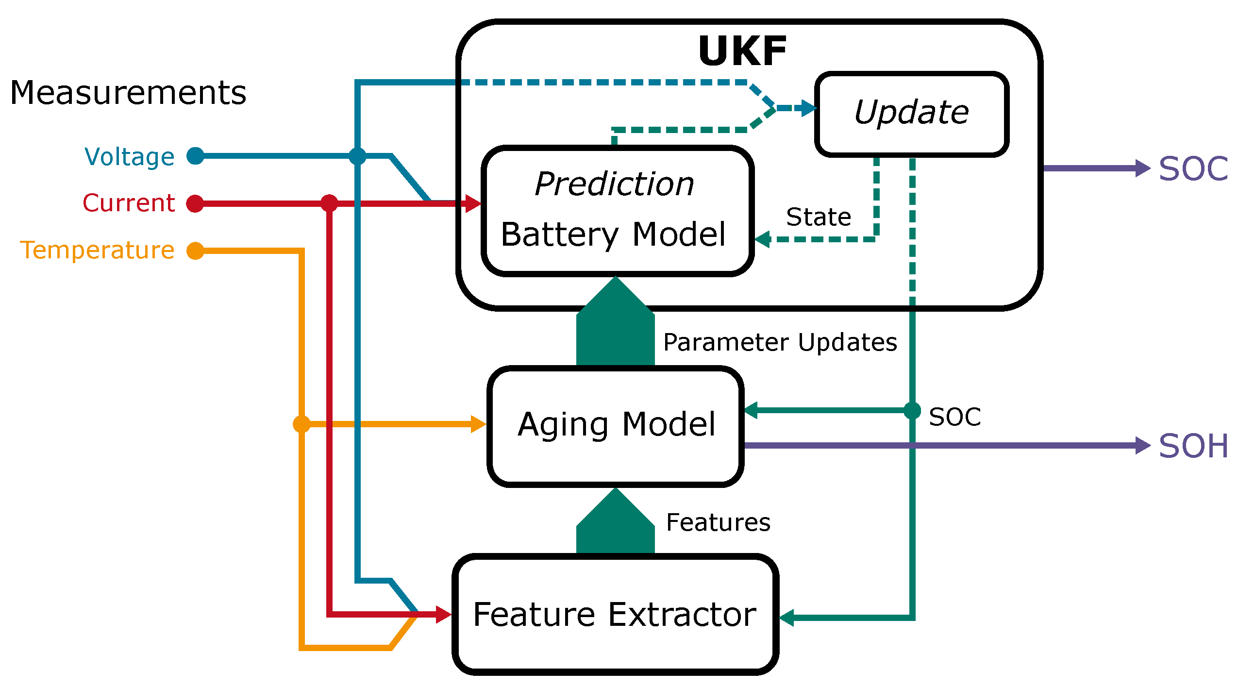
1.6. System Description

The system developed in this work starts with the measurements, where the current is used to predict the states of the system by using the battery model and the voltage to update the states inside the SOC estimation, where the UKF is used. The conducted measurements are described in Section 2. The battery model depends on the different parameters of the dynamic model; these parameters depend on the SOH, the temperature, and the SOC. The UKF and the model belong to the SOC estimation and are described in Section 3. By analysing the measurements and the SOC, the features that describe the stress factors during ageing are calculated using the feature extractor. The feature extraction and the ageing model belong to the SOH estimation in Section 4. The condensed stress factors are forwarded into the ageing model, which works on one hand as a parameter model, describing the SOC and temperature-dependent behaviour. On the other hand, the ageing model describes the SOH based on stress factors. The parameters are updated in every iteration for SOC and temperature dependencies and, when it is issued, by the feature extractor for the SOH dependence. By running iteratively through the measurements of the SOC, the features and the SOH are estimated for every sample. Figure 1 displays a schematic of the system.

2. Measurements and Dataset

The dataset consists of 30 cells called HE4 from LG Chem aged in a hybrid ageing manner, so no differentiation between calendar or cycle ageing was made. The specifications of the cell are displayed in

Table 1. Cell specifications.

Specification	Value
Nominal Capacity	$2.5 \mathrm{A} \mathrm{h}$
Nominal Voltage	$3.6 \mathrm{V}$
Final Discharge Voltage	$2.5 \mathrm{V}$
Charging End Voltage	$4.2 \mathrm{V}$
Maximum Constant Discharge Current	$20 \mathrm{A}$
Maximum Charging Current	$4 \mathrm{A}$

.

The battery cells were aged under different stress factors considering three temperatures (room temperature (23 °C), 25 °C, and 45 °C), three different mean SOCs, and three different DODs. Different currents are not considered during constant current ageing. In addition, it includes two cells aged under dynamic conditions at room temperature (23 °C).

Table 2. Table of the different stress factors considered in the ageing measurements.

Temperature (°C)	DOD	${\mathbf{SOC}}_{\mathbf{mean}}$	Number of Cells	Cyclic Ageing
25	1	0.5	4	Constant current
25	0.3	0.35	4	Constant current
25	0.3	0.65	4	Constant current
45	1	0.5	4	Constant current
45	0.3	0.35	4	Constant current
45	0.3	0.65	4	Constant current
23	0.7	0.5	2	Constant current
23	0.3	0.5	2	Constant current
23	1	0.5	2	Dynamic profile

sums up the different stress factors and displays the stress factor matrix.

The ageing is frequently interrupted by a battery cell capacity test, every ten full-cycle equivalents, and less frequently by a full characterisation. During the ageing process, the battery cells are cycled using constant current for charging and discharging, except for the two dynamically aged cells.

The characterisation is taken out at the specific ageing temperature since the outer mean SOC and DOD combinations are conducted at the two temperatures. The check-up characterisations consist of a capacity test, a hybrid of an incremental open circuit voltage, and a slightly adjusted hybrid pulse power characterisation (HPPC). Pre-tests have shown that the influence of the HPPC on the OCV is negligible. Furthermore, the incremental method is an exact and time-efficient way of measuring the OCV and being able to perform additional analysis, namely, differential voltage analysis [31]. The increments in OCV are based on every percent of the nominal capacity and the HPPC at every ten percent. The measurement equipment used consisted of a Neware battery cycler with a voltage range of 10 $\mathrm{V}$ and $\pm 10 \mathrm{A}$ and either a Memmert oven for the 45 °C or a temperature chamber from Binder for the 25 °C measurements. The check-up was extended for the two dynamically aged cells with a validation part, including dynamic discharges and constant current constant voltage (CCCV) charging procedures. Figure 2 displays the used check-up and validation extension.

For the dynamic ageing, the federal urban driving schedule was applied to a battery cell of the same type, so the cell was CCCV charged and then discharged to 2.5 V using the FUDS repeatedly. This measurement was used to design dynamic parts of the ageing. To generate these parts, the so-called random pulse method was used to create profiles of defined length, as explained in [32]. The general process comprises segmenting the measured current profiles in charging and discharging pulses and saving them to a database. Afterwards, the pulses are selected randomly and added to the profile. Even without actual driving data, a dynamic profile with random pulse sequences is generated that is ready to be used during the cyclic ageing of the cells. The cycling includes short cycles of 25%, 30%, 75%, 80%, and 95% DOD. These cycles are concatenated to sum up to about ten full-cycle equivalents followed by a capacity test (see Figure 3).

3. SOC Estimation

For the SOC estimation, a model-based approach is employed that is part of the Kalman filter family. The Kalman filters are a widespread family of filters used for state estimation. The general Kalman filter is the simplest of the filters. It recursively uses the system described in state space and the measurements to estimate the state. By weighting the prediction and the measurement, the Kalman filter can account for noise, variations in the measurement, and inaccuracies of the used model. Since it is based on the Bayesian filter, it considers the state to be a normal Gaussian distribution described by its mean and the variance or covariance matrix for multiple dimensions. So, by using the model for the prediction, a Gaussian distribution is estimated based on its last state and the model’s behaviour described by the state space equations. Uncertainties are added to account for model and measurement imperfections. The measurement represents another Gaussian distribution, and by multiplying the prediction with the measurement, a new distribution can be calculated. By extracting the so-called Kalman gain, the new state can be estimated. Figure 4 summarises the mentioned steps.

The Kalman filter is not feasible for battery state estimation since it only operates with a linear system, which is not the case for battery models and would lead to errors during estimation. Different variants have been developed [3,12,13,14].

The extended Kalman filter (EKF) is one variant that linearises the current mean and the covariance with a Taylor series approximation in every step to nullify the nonlinearities. In general, the EKF uses the same framework of time update and measurement update but calculates each time the Jacobian matrix of partial derivatives of the nonlinear state equation for the state and the process noise and Jacobian matrix of partial derivatives of the measurement equation for the state and the measurement noise. The problem with this kind of linearisation is that the distributions of random variables are no longer normal after the nonlinear transformation. Often the EKF is used to estimate the SOC using an ECM or the SOH based on estimating the capacity and internal resistance [14,17,33,34].

Another variant of approaches, generalized as sigma-point Kalman filters (SPKFs), handles the nonlinear problem using a statistical approach. So, the SPKF uses multiple sigma points depending on the dimensions of the state vector. For these points, the time and measurement update is calculated, which means they are all transformed, and afterwards, they are all used to estimate the current state vector. The advantage is that this filter does not calculate Jacobians or Hessians without losing information and precision. SPKFs are differentiated based on the selection rule of the sigma points in the central difference Kalman filter, unscented Kalman filter, or cubature Kalman filter [3,14,17,33,35,36]. However, to use a model-based approach, a model is a central part of estimating the SOC.

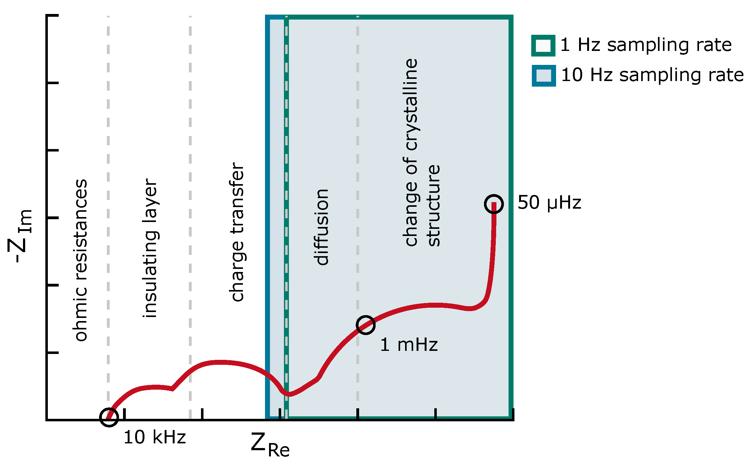
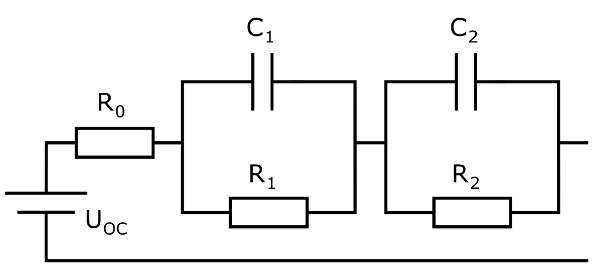
3.1. Dynamic Model Description

The modelling of a system has multiple purposes. It supports the design, analysis, verification, or validation of a system. In the case of BMS, it serves the purpose of analysing the system in terms of diagnosing and prognosing the actual state of the battery system. In the case of the model-based approach for SOC estimation, the model is used to calculate the prediction, which is necessary to estimate the system’s internal state. Different modelling approaches can be physio-chemical, equivalent circuits, or mathematical models. The data that can be measured is essential, and on the other hand, how efficient is the computation of the model?

Depending on the purpose, the model differs by the information needed to build the model. They are often divided into black box and white box models. Black box models do not need any system knowledge to model the behaviour. They are often represented by empirical or mathematical models. In contrast, white box models are based on describing the processes that lead to the specific behaviour of the system. These models could consist of multiple differential equations. In other words, white box models are based on knowledge, whereas black box models are based on data to represent the system’s behaviour. The hybrid of these models is called the grey box model and uses both the knowledge and data-based approaches to model the system’s behaviour. This approach helps to model a system where some parts of the internal processes are known, and others are not. It is also used to simplify a model to reduce its complexity and focus on parts where a diagnosis should be possible.

In terms of battery models, the different categories of models lead to electrochemical models (white box), data-driven models such as neural networks (black box), or equivalent circuit models with additional empirical models to reproduce the behaviour of battery cells.

The base of most electrochemical battery models is formed by the work by Doyle, Fuller, and Newman described in [37]. They describe the model as having a one-dimensional transport from the anode to the cathode, passing the polymer separator. Film formation at the lithium/polymer interface is discarded to keep the complexity manageable. At the same time, the transport is modelled via the concentrated solution theory, leading to a binary electrolyte and a polymer solvent with one phase. Therefore, the transport in the electrolyte is defined by the electrical conductivity, the transference number, and the diffusion coefficient. These parameters depend on the concentration and could lead to different physical properties. By doing so, the transport phenomena can be handled [37]. All in all, it is described such that it leads to a pseudo-two-dimensional problem based on a one-dimensional problem on the micro- and macro-scales [38]. Since the process is nonlinear and pseudo-two-dimensional, it results in an issue that is only numerically solvable and, therefore, unsuitable for every task such as parameter estimation [38].

For further usage, the Doyle–Fuller–Newman model is simplified to form the so-called single-particle model, which assumes a uniform reaction rate across the electrodes and neglects the electrolyte dynamics [39]. Using these assumptions, the electrodes are modelled as single particles [40]. Electrochemical models can be used in applications such as SOH estimation based on that simplification. Further improvements have been made to represent degradation based on solid electrolyte interface development, cracking, and handling electrolyte dynamics [40,41,42]. However, they are still represented by complex differential equations with many parameters.

Electrochemical models are mostly either single-particle models or pseudo-two-dimensional models, which are mainly used for design and analysis because they need detailed information on the battery structure, the materials, and the electrolyte [43]. They have also been used for state estimation in some cases [44,45]. Nevertheless, they are complex and lack usability when the information on the battery cell is limited.

Data-driven models include every kind of mathematical model that can be used to reproduce the behaviour of a battery cell. They can be built up from neural networks, support vector machines, fuzzy-logic-based, or others. These models are often called black box models since they do not deliver an analytical insight; their parameters are not relatable to the system that should be modelled. However, they can have a good performance computationally and error-wise. They can be used for monitoring, diagnostics, design, and understanding physical phenomena. Nevertheless, depending on the application task, the correct data to train the model is needed, which can be very time-consuming since the data-driven models tend to overfit the data and cannot extrapolate the data to states beyond the training data [6,36,46]. The widely used equivalent circuit models (ECMs) can represent the dynamic behaviour resulting from the reaction’s electrochemical processes during charge or discharge. Depending on the application, the ECM is employed as a straightforward model that is computationally efficient [47,48]. Two different approaches for ECMs try to emulate the battery behaviour using mostly common electrical components such as resistors, capacitors, and voltage sources. Their aim differs to a small extent, since one approach is completely empirical and the other aims to model the behaviour with electrochemical relations—the difference in the model generation lies in the underlying measurements. ECMs with electrochemical relations start with electrochemical impedance spectroscopy (EIS) measurements, and most empirical ECMs start with pulse measurements.

The laboratory measurements during testing included a capacity test, an OCV, and pulse measurements. For electrochemical models, invasive measurements are needed. Nevertheless, it is still possible to identify the parameters of an ECM and data-driven models.

Overall, ECMs promise good computability, interpretability, and efficiency with a reasonable amount of parameters, and, furthermore, they are often used in combination with model-based state estimation approaches.

The boundary conditions must be considered when designing an ECM for a specific application. That means, which measurements can be taken, which data can be collected, where the model should be used, and what is expected of the model. Following the literature on the next steps of a BMS, it is the online diagnostics of battery cells, identifying which processes lead to the current behaviour of the cell. Hence, the literature on modelling for BMS usage seeks for at least a potent physics-based ECM [36] or even reduced-order models of electrochemical models [40,44,45]. For most physics-based ECMs, at least EIS measurements are needed. Speaking of the boundary conditions in an application, the measurements’ sampling rates and resolutions are the most important for the model design and the parameter estimation. Since no specific measurement schemes are taken in an application, the boundary conditions reduce further to the resolution and rate. The resolution in a BMS ranges from 8 bit to 16 bit, hence, theoretically, for a measurement in the range of 0 $\mathrm{V}$ to 5 $\mathrm{V}$ from $9.8$ $\mathrm{m}$$\mathrm{V}$ to 38 μV accuracy, but considering the noise from 16 mV to 300 μV accuracy [49]. The sampling rate that is applied in electric vehicles depends on whether it is a high-power application, where a faster rate is needed, or a high-energy application, where a slower rate is feasible. Nevertheless, the rates range from 1 s⁻¹ to 10 s⁻¹ [49]. Specifically looking at the sampling rate, the number of electrochemical processes that can be investigated shrinks. Taking account of the sampling rate, the following Figure 5 displays the electrochemical processes that can be modelled by showing the EIS, which includes a small part of the charge transfer, the diffusion, and the change in crystalline structure. This figure does not take the Nyquist–Shannon sampling theorem into account.

Different ECMs are still usable, considering the impedance spectra and sampling rate. They can be of fractional order or can include multiple RC elements. These models can be lumped. Since the paper’s main focus is not the modelling, the model used is a typical two-RC model with an OCV part. This model is often used when a model-based state estimation approach is followed [50,51], even of a lower order [33,52]. Overall the two-RC model is able to model the EIS of a lithium-ion battery. Therefore, it is suitable to be used as a model for the SOC estimation and the representation of the battery cell in the case of dynamic battery cell behaviour.

3.1.1. Dynamic Model Equations and Discretisation

This section states the model equations and their discretisation for the dynamic battery cell model. The model is displayed in Figure 6. The differential equation describing the model can be established by using Kirchhoff’s and Ohm’s laws and considering that $\tau =R·C$.

$$U\left(t\right)=U_{OC}\left(t\right)+U_0\left(t\right)+U_1\left(t\right)+U_2\left(t\right)$$

(4)

$$U\left(t\right)=U_{OC}\left(t\right)+R_{0}i\left(t\right)+R_{1}i\left(t\right)-{\tau }_1\frac{\mathrm{d}{U}_1\left(t\right)}{\mathrm{d}t}+R_{2}i\left(t\right)-{\tau }_2\frac{\mathrm{d}{U}_2\left(t\right)}{\mathrm{d}t}$$

(5)

For the next step to obtain the equations needed, the differential equation is Laplace-transformed using the law of linearity, leading to

$$U\left(s\right)=U_{OC}\left(s\right)+R_{0}i\left(s\right)+\frac{R_1}{1+{\tau }_{1}s}i\left(s\right)+\frac{R_2}{1+{\tau }_{2}s}i\left(s\right).$$

(6)

By applying the bilinear transformation

$$s=\frac{2}{T}\frac{1-z^{-1}}{1+z^{-1}}$$

(7)

and discretising every term on its own leads to the following results.

$$Z\left\{U_{OC}\left(s\right)\right\}=U_{OC}\left(z\right)$$

(8)

$$Z\left\{U_0\left(s\right)\right\}=Z\left\{R_{0}i\left(s\right)\right\}=R_{0}i\left(z\right)$$

(9)

$$\begin{array}{cc}\hfill Z\left\{U_1\left(s\right)\right\}& =Z\left\{\frac{R_1}{1+{\tau }_{1}s}i\left(s\right)\right\}\hfill \\ \hfill & =\frac{R_1}{1+\frac{2}{T}{\tau }_1}i\left(z\right)+\frac{R_1}{1+\frac{2}{T}{\tau }_1}i\left(z\right)z^{-1}-\frac{1-\frac{2}{T}{\tau }_1}{1+\frac{2}{T}{\tau }_1}{U}_1\left(z\right)z^{-1}.\hfill \end{array}$$

(10)

$$\begin{array}{cc}\hfill Z\left\{U_2\left(s\right)\right\}& =Z\left\{\frac{R_2}{1+{\tau }_{2}s}i\left(s\right)\right\}\hfill \\ \hfill & =\frac{R_2}{1+\frac{2}{T}{\tau }_2}i\left(z\right)+\frac{R_2}{1+\frac{2}{T}{\tau }_2}i\left(z\right)z^{-1}-\frac{1-\frac{2}{T}{\tau }_2}{1+\frac{2}{T}{\tau }_2}{U}_2\left(z\right)z^{-1}\hfill \end{array}$$

(11)

The bilinear transformation is applied due to its stability and time-domain accuracy advantages, which were tested in a simulation beforehand. Using the equations and transforming them to the discrete-time domain, and formulating them in state space, leads to a model that state estimation algorithms can handle:

$$\left[\begin{array}{c}SOC\left(k\right)\\ U_1\left(k\right)\\ U_2\left(k\right)\end{array}\right]=\left[\begin{array}{ccc}1& 0& 0\\ 0& \frac{1-\frac{2}{T}{\tau }_1}{1+\frac{2}{T}{\tau }_1}& 0\\ 0& 0& \frac{1-\frac{2}{T}{\tau }_2}{1+\frac{2}{T}{\tau }_2}\end{array}\right]\left[\begin{array}{c}SOC(k-1)\\ U_1(k-1)\\ U_2(k-1)\end{array}\right]+\left[\begin{array}{cc}\frac{1}{C_N}& 0\\ \frac{R_1}{1+\frac{2}{T}{\tau }_1}& \frac{R_1}{1+\frac{2}{T}{\tau }_1}\\ \frac{R_2}{1+\frac{2}{T}{\tau }_2}& \frac{R_2}{1+\frac{2}{T}{\tau }_2}\end{array}\right]\left[\begin{array}{c}i\left(k\right)\\ i(k-1)\end{array}\right]$$

(12)

$$\begin{array}{cc}\hfill U\left(k\right)& =U_{OC}\left(SOC\left(k\right)\right)+U_1\left(k\right)+U_2\left(k\right)+R_{0}i\left(k\right).\hfill \end{array}$$

(13)

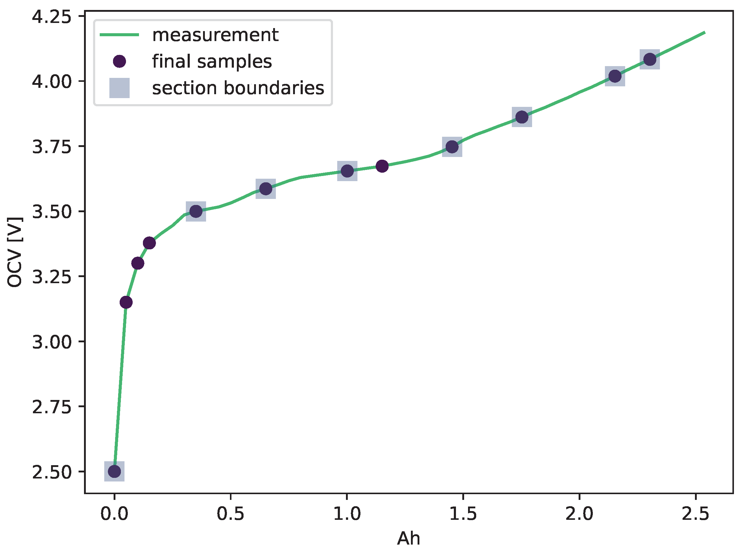
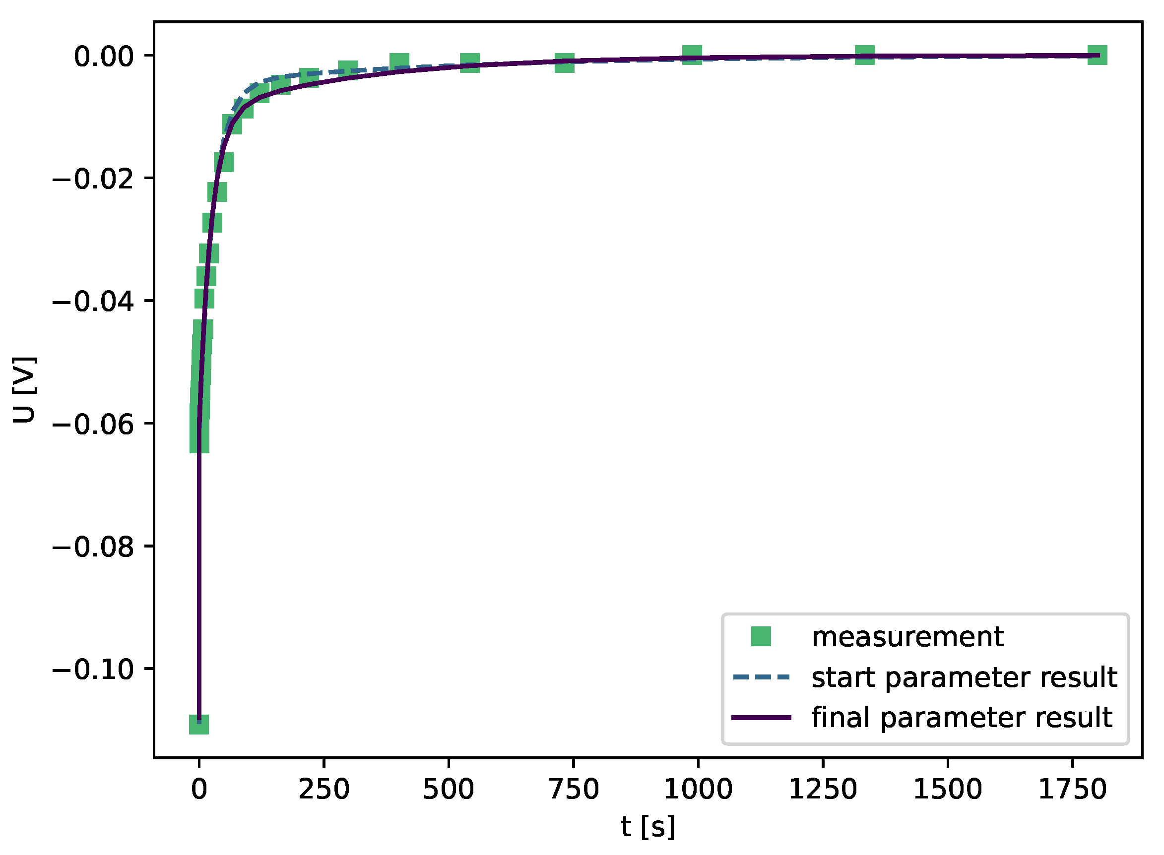
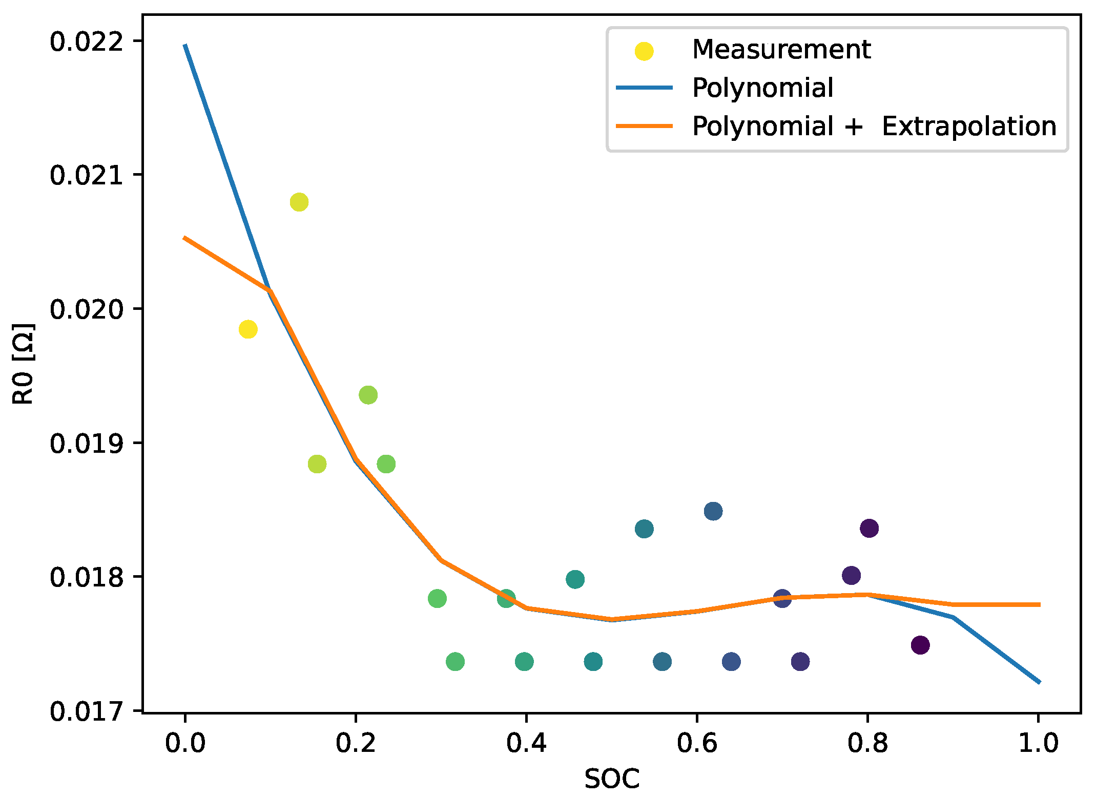
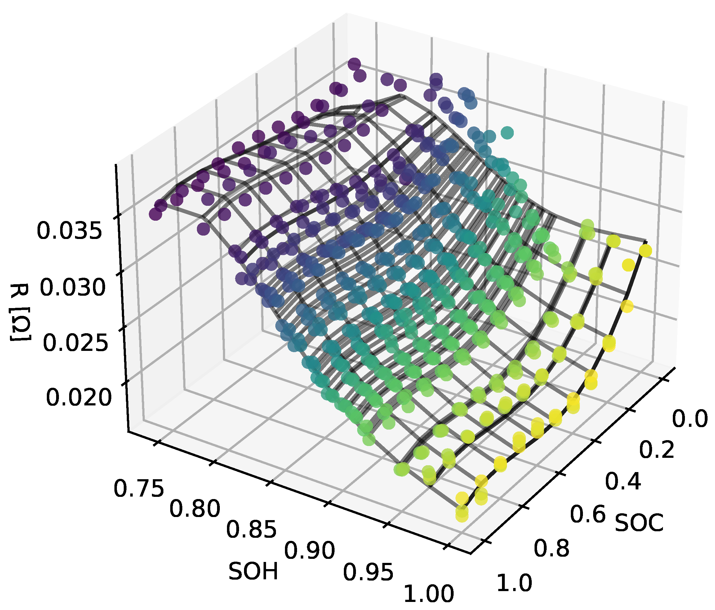
3.1.2. Parameterisation

Parameterisation is the process of extracting the model’s parameters from the measurements. To be able to extract the parameters, every ageing cycle is frequently interrupted by a check-up. Every check-up is preprocessed to obtain the measurement’s capacity, the OCV, and the pulses. Before preprocessing, the measurements are imported and formatted into a universal format because only the import function has to be changed if the saved measurement file changes. The capacity is calculated from the 1C discharging; a CCCV charge precedes that. Another CCCV charge follows this discharge and the hybrid test phase of the incremental OCV and the HPPC pulse test. The OCV in the charging and discharging directions can be estimated from the hybrid phase; see Figure 2 for an example of the check-up. During the preprocessing, the check-up data, in a standardised import data format, is separated into different parts, starting from the OCV voltages extracted from the hybrid part from the resting phase of the incremental OCV to the relaxations of the HPPC pulses that are used to determine the dynamic parameters of the battery model, the battery internal resistance, the resistances of the RC elements, and its time constants. By using the pulse relaxation, the change in OCV does not have to be included because there is none during the relaxation. Furthermore, the capacity is directly extracted from the 1C discharging, and the validation is extracted as well if present. The validation part is only present for cells aged under dynamic regimes.

Open Circuit Voltage Modelling

The OCV is a central part of the model since it describes the midterm behaviour of a battery if the battery behaviour is segmented into short-term, dynamic behaviour, mid-term, OCV behaviour, and long-term, described by the ageing behaviour. There are different approaches to modelling the OCV in the literature, ranging from tables to empirical models such as polynomials or more electrochemical-based models [53,54,55,56]. For more information on different models for OCV modelling, please refer, for example, to Pillai et al. [56]. To model the OCV, a table-based approach will be used, which can lead to a stable and easy method to represent the OCV when sampled correctly. The approach is based on the inflection point method described by Sundaresan et al. [53]. A few changes were added to the sampling to improve the performance. The following steps were followed to sample the measured OCV curve:

• Calculation of the signed curvature of the OCV according to Narula [57]

  $$\kappa \left(x\right)=\frac{x^{″}{y}^{\prime }-x^{\prime }{y}^{″}}{{({\left(x^{\prime }\right)}^2+{\left(y^{\prime }\right)}^2)}^{3/2}}$$

  (14)
• Find roots of the curvature to segment the OCV. Therefore, calculate

  $$\kappa \left(x\right)=0$$

  (15)

  to obtain the roots. Add the first measurement point and roots to the samples.

  $$\begin{array}{c}\hfill samples=[x\left(0\right),{\kappa }_{roots},x\left(end\right)]\end{array}$$

  (16)
• Delete the inner samples if the section range is lower than 5% of the SOC for minimum section size.
• Allocate the samples equally to the sections.
• If there are still samples left:

  (a)

  Calculate the error and curvature peaks per section;

  (b)

  Add a sample to the section with the highest error;

  (c)

  Distribute samples equidistantly in sections;

  (d)

  Go to 5.

• Finished sampling the OCV.

The main differences to Sundaresan et al. [53] is the formula for calculating the curvature and the steps to distribute the samples, despite the equal distribution. Because the approach described in the literature could lead to many samples in just two sections, even if other sections would benefit from additional samples, this distribution depends on the number of excess samples after the equal distribution. If no samples are left, the distribution of the excess samples is not conducted. Figure 7 displays the result of the sampling compared to the measurement.

Dynamic Parameter Identification

The battery model’s dynamic parameters are the battery cells’ ohmic resistance, the resistances belonging to the RC elements, and the time constants. The time constants are used instead of the RC capacities because they are simpler for identifying boundaries, and the distribution of relaxation times could be easily used for estimation of the start parameters. The relaxation of the HPPC part of the check-up is used to identify the parameters. Identifying the parameters is divided into the preprocessing of the relaxation, the estimation of the start parameters, and the fitting itself. The relaxation consists of switching from the current pulse to the relaxation and the complete relaxation. The measurement is checked for doubled data points and NaNs during preprocessing. Afterwards, the relaxation is freed from the OCV by subtracting the last voltage of the relaxation. Because the relaxation is 1800 s long and sampled every $0.1$ $\mathrm{s}$, it consists of many samples and many of these samples are part of the relaxed voltage. Many samples in this area work during the fitting process as a weighting since the faster processes should be fitted as well. Logarithmic resampling was used to have more samples at the beginning of the relaxation and fewer at the end.

Estimating the start parameters is essential; the better the start parameters, the better the fit. In this case, estimating the start parameters is relatively complex. The overall process consists of different steps starting with the estimation of the ohmic series resistance using

$$R_0=\frac{U(t=0.3 \mathrm{s})-U(t=0 \mathrm{s})}{I(t=0.3 \mathrm{s})-I(t=0 \mathrm{s})}.$$

(17)

Then, the next step includes estimating the resistances and time constants of the RC elements. This step includes calculating the so-called distribution of relaxation times (DRT) to obtain meaningful parameters. Since no electrochemical impedance spectroscopy was measured, the DRT is estimated by overfitting the relaxation with five RC elements, calculating the impedance spectra using the fitted parameters and the impedance equation, and calculating the DRT using the package pyDRTtools by Wan et al. [58]. The DRT is evaluated for local peaks, whether they lie in the range of the boundaries used for fitting the parameters later on. If they lie in the range of one of the ranges of the time constants, the time constant is used as the starting parameter of the specific RC element time constant. The resistance corresponding to the respective time constant is calculated by

$$U_{RC,1}=U_{pp}(t=0)-U_{pp}(t=5{\tau }_{RC,1})$$

(18)

$$R_{RC,1}=U_{RC,1}/I_{pulse,t=0}$$

(19)

for the first and the other RC elements

$$U_{RC,n}=U_{pp}(t=5{\tau }_{RC,n-1})-U_{pp}(t=5{\tau }_{RC,n})$$

(20)

$$R_{RC,1}=U_{RC,n}/I_{pulse}(t=0).$$

(21)

where $U_{pp}$ is the preprocessed measured relaxation voltage, $R_{RC,n}$ is the resistance, and ${\tau }_{RC,n}$ is the time constant of the n-th RC element. At this point, the start parameter estimation is finished. For robustness, the start parameters for time constants are the mean of their boundaries if no peak in the region of the boundaries is found.

Now, the data are fitted using the lmfit package by Newville et al. [59], applying the minimizer with the Nelder–Mead algorithm. Only the parameters of the RC elements are fitted, and the ohmic resistance is kept constant throughout the fitting process. Because the fitting is performed on a relaxation process, the fitted model has to include the starting voltage of the RC elements, because instead of having 0 $\mathrm{V}$ at the RC element, the capacity is pre-charged by the previous current pulse. Therefore, the discrete equation for a single RC element itself is as follows.

$$\begin{array}{cc}U{\left[k\right]}_{RC,n}=e^{\frac{-t\left[k\right]}{{\tau }_{RC,n}}}U{[k-1]}_{RC,n}+R_{RC,n}I\left[k\right]\left(1-e^{\frac{-t\left[k\right]}{{\tau }_{RC,n}}}\right),\hfill & \hfill k=[1,size(t\left)\right]\end{array}$$

(22)

$$\begin{array}{cc}U{\left[k\right]}_{RC,n}=R_{RC,n}I\left[k\right](1-e^{\frac{-t_{pulse}}{{\tau }_{RC,n}}}),\hfill & \hfill k=0\end{array}$$

(23)

See Figure 8 for a start parameter result and a fitting result.

These processes are applied to every check-up and the extracted relaxations.

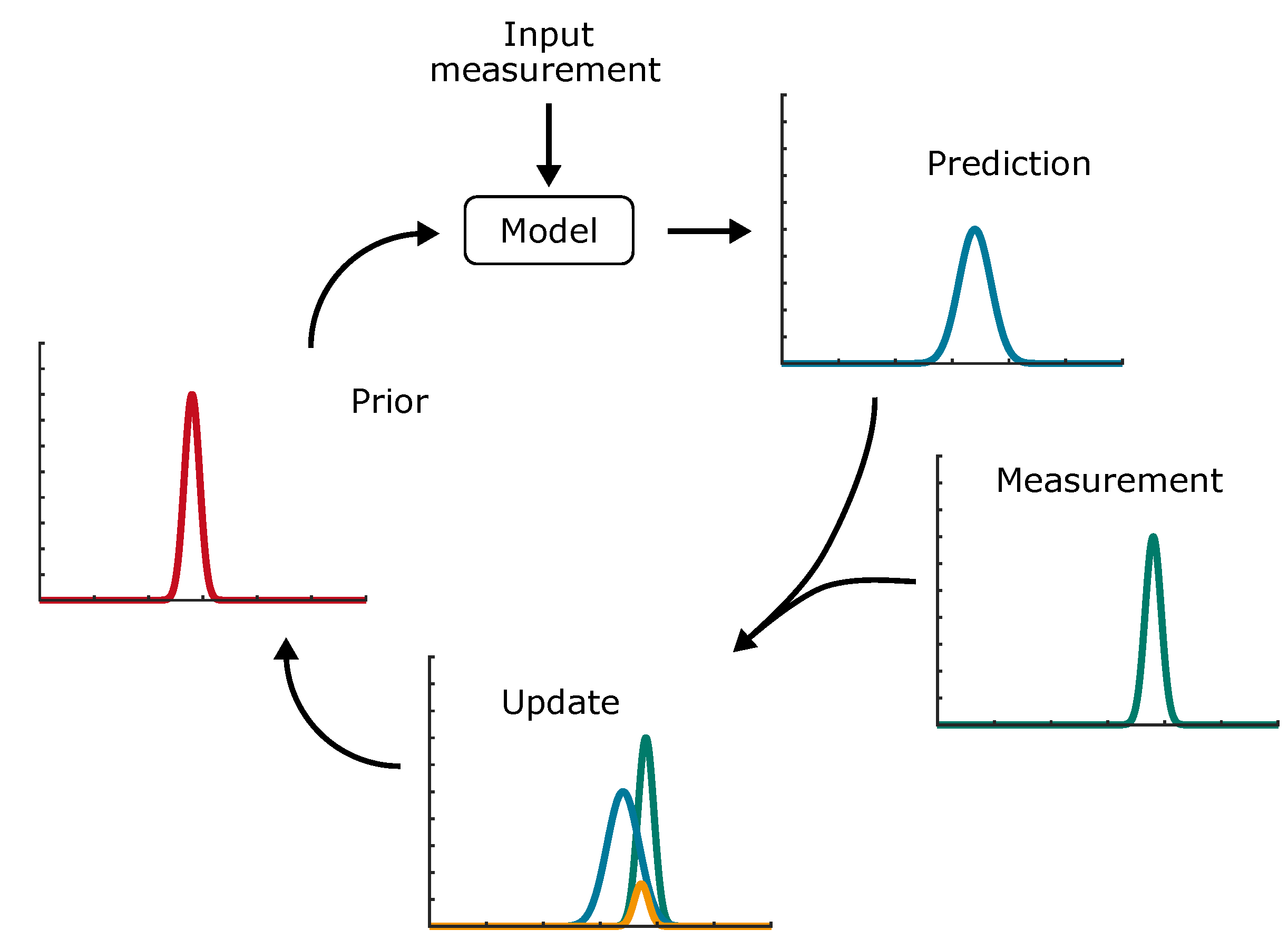
3.2. Unscented Kalman Filter

In general, the UKF follows the same process as other filters, including the prediction and update steps. Of course, these steps can be further divided into smaller substeps. Its name is derived from the unscented transform, an approach used for the statistical calculation of random variables that undergo a nonlinear transformation. Instead of calculating the Jacobian and Hessian matrices, the UKF uses discrete samples, called sigma points, that are projected through the transformation. By using weights, the mean and the covariance can be calculated [60,61]. The general process is described here:

• Initialization of the mean and the covariance with expectations, where x is the state vector.

  $${\widehat{x}}_0=\mathbb{E}\left[x_0\right]$$

  (24)

  $$P_0=\mathbb{E}\left[(x_0-{\widehat{x}}_0){(x_0-{\widehat{x}}_0)}^T\right]$$

  (25)
• Prediction of the current state, including sampling and weight calculation.

  (a)

  Calculate the sigma points based on the mean ${\widehat{x}}_{k-1}$, depending on the dimension of the state vector and mean N, using the composite scaling factor $\lambda$:

  $$\begin{array}{c}{\mathcal{X}}_{k-1,i}=\left\{\begin{array}{cc}{\widehat{x}}_{k-1}\hfill & ,i=0\hfill \\ {\widehat{x}}_{k-1}+\sqrt{(N+\lambda )P_{k-1}}\hfill & ,i=1,\dots N\hfill \\ {\widehat{x}}_{k-1}-\sqrt{(N+\lambda )P_{k-1}}\hfill & ,i=N+1,\dots 2N\hfill \end{array}\right.\hfill \end{array}$$

  (26)

  where the scaling factor is

  $$\lambda ={\alpha }^{\beta }(N+\kappa )-N$$

  (27)

  with $\alpha$ determining the spread of the samples, $\beta$ depends on the expected type of distribution, where for a Gaussian $\beta =2$, and $\kappa$ being the scaling factor, which is usually equal to $3-N$.

  (b)

  Transform the samples using the model system equation $\left(F\right)$ and the input (u)

  $${{\mathcal{X}}^{*}}_k=F({\mathcal{X}}_{k-1},u_{k-1}).$$

  (28)

  (c)

  Calculate the predicted mean ${\widehat{x}}_k^{-}$ and covariance based on the samples by using the weights $W_{m,i}$ for the mean and $W_{c,i}$ for the covariance in addition to the process noise covariance $R^p$

  $${\widehat{x}}_k^{-}=\sum _{i=0}^{2N}{W}_{m,i}{{\mathcal{X}}^{*}}_k$$

  (29)

  $$P_k^{-}=\sum _{i=0}^{2N}{W}_{c,i}({{\mathcal{X}}^{*}}_k-{\widehat{x}}_k^{-}){({{\mathcal{X}}^{*}}_k-{\widehat{x}}_k^{-})}^T+R^p$$

  (30)

  and augment the samples with additive noise

  $${\mathcal{X}}_{k,i}=\left\{\begin{array}{cc}{{\mathcal{X}}^{*}}_{k,i}\hfill & ,i=0,\hfill \\ {{\mathcal{X}}^{*}}_{k,i,0}+\sqrt{(N+\lambda )R^p}\hfill & ,i=1,\dots N,\hfill \\ {{\mathcal{X}}^{*}}_{k,i,0}-\sqrt{(N+\lambda )R^p}\hfill & ,i=N+1,\dots 2N.\hfill \end{array}\right.$$

  (31)

  (d)

  Calculate the output with the output equation of the model (H) using the samples and calculate its mean with the weights:

  $${\mathcal{Y}}_k=H\left({\mathcal{X}}_k\right),$$

  (32)

  $${\widehat{y}}_k^{-}=\sum _{i=0}^{2N}{W}_{m,i}{\mathcal{Y}}_{k,i}$$

  (33)

• The measurement update calculates the new state of the model using the prediction, the Kalman gain, and the measurement of the output. Furthermore, the measurement noise is added.

  (a)

  Calculate the Kalman gain:

  $$P_{yy,k}=\sum _{i=0}^{2N}{W}_{c,i}({\mathcal{Y}}_{k,i}-{\widehat{y}}_k^{-}){({\mathcal{Y}}_{k,i}-{\widehat{y}}_k^{-})}^T+R^m$$

  (34)

  $$P_{xy,k}=\sum _{i=0}^{2N}{W}_{c,i}({\mathcal{X}}_{k,i}-{\widehat{x}}_k^{-}){({\mathcal{Y}}_{k,i}-{\widehat{y}}_k^{-})}^T$$

  (35)

  $$\mathcal{K}=P_{xy,k}{P}_{yy,k}^{-1}.$$

  (36)

  (b)

  Calculate the state and covariance of the state of the model using the Kalman gain and the measurement of the output ($y_k$):

  $${\widehat{x}}_k={\widehat{x}}_k^{-}+\mathcal{K}(y_k-{\widehat{y}}_k^{-})$$

  (37)

  $$P_k=P_k^{-}-\mathcal{K}{P}_{yy,k}{\mathcal{K}}_k^T.$$

  (38)

  (c)

  After the calculation of the current state, it is shifted to be the old state (${\widehat{x}}_{k-1}$), and the same is performed for the covariance ($P_{k-1}$). Now, start all over again with the prediction steps, and so on.

These process steps are applied to the model described in Section 3.1 to estimate the internal cell states of the model consisting of the SOC and the overpotentials of the two RC elements. Due to instability outside the defined state boundaries, especially for the SOC, because it influences different parts of the model, the states are bounded at low and high SOCs. Otherwise, the Kalman filter deconverges fast. Now, the state estimation consists of the SOC estimation based on the model using the UKF. It is extended by an SOH estimation based on an ageing model.

4. SOH Estimation

As for the SOC estimation, the SOH estimation can be grouped into direct measurements, model-based, and data-driven approaches. Direct measurements for the SOH estimation consider an analysis based on the relation of the OCV and the SOC, where slight changes over the degradation are identified. The analysis is called incremental capacity analysis (ICA) and describes the differentiation of the charge over the voltage that leads to peaks in the region of phase changes. The ICA is calculated from current measurements at constant currents for a full or a partial discharge/charge cycle. The battery cell’s SOH can be estimated by tracking the position, amplitude, and enveloped area [12,13]. Of course, the change in these peaks has to be investigated prior to the application to know which change belongs to which SOH. Another direct approach is the so-called cycle counter. Based on the coulomb counter, a cycle counter could be established that counts the equivalent full cycles during usage. Therefore, it is extended such that it only counts the charge in the charge direction or the absolute value of the current in both the charging and discharging directions and is divided by either the capacity or two times the capacity. To be able to use this information correctly, many measurements have to be conducted to obtain the relation between several equivalent full cycles and the SOH, because the trajectory of the degradation highly depends on stress factors such as the current rate, the temperature, the $\Delta$DOD, and the mean voltage. Another approach is to use the relation of the internal resistance with the ageing processes. This derives the SOH based on the measurement of the internal resistance either from EIS measurements or pulses. The next group of methods includes model-based approaches, divided into direct and indirect approaches, where direct models that are used for direct estimation are, for example, semi-empirical, empirical, and electrochemical ageing models used to estimate the SOH. Empirical and semi-empirical models are developed based on ageing measurements considering different stress factors. The model is fitted to the change in a parameter over time, or full-cycle equivalents, i.e., the internal resistance or the capacity, and is used to calculate the current SOH or RUL considering the cycles or the time at a specific stress factor. A weighted coulomb-counter-based cycle counter can be used to track the influence of stress factors. The same approach can be used if the empirical model is replaced with the degradation data saved in a characteristic map [12,13,15]. By using a more sophisticated model such as an electrochemical pseudo-two-dimensional model and different ageing improvements, the extrapolation ability and, therefore, the prediction ability is improved for unseen data. In addition, the model could be able to diagnose the ageing process. However, due to their complexity and the involvement of many parameters and multiple partial differential equations, such models are unsuitable for online usage. Therefore, research focuses on simplifications and parameterisation [12,13]. Model-based approaches that incorporate models are, in most cases, observers and filters. The model is used to predict the measurement, where the model’s state consists of its parameters and not its SOC or overpotential [6,14,33,34]. In the group of data-driven approaches, some parts of the direct models can be used since they rely highly on data or machine learning approaches, such as the support vector machine or neural networks. These algorithms can be used to directly estimate the SOH based on measurements such as EIS or charge profiles that are measured during the application [3,12,13,62]. A much more specialised approach for sequential data is the recursive neural network (RNN). One central part of an RNN is parameter sharing, meaning that parameters are shared between multiple parts of the model. The second central part is that the network has connections to results in the past. Therefore, the present values of a variable can influence its future values. Different approaches are considered to be RNNs [63]. These models are often used for RUL prediction and capacity degradation prediction in general.

For this work, the decision is made to use a direct model-based approach, where an ageing model is designed based on the measurements made and a cycle counter is used to access the model. This approach is common and sometimes extended with a filter or observer. The following sections describe the processing of the raw ageing data into combined datasets and, from there, the ageing model and its usage in combination with the cycle counter.

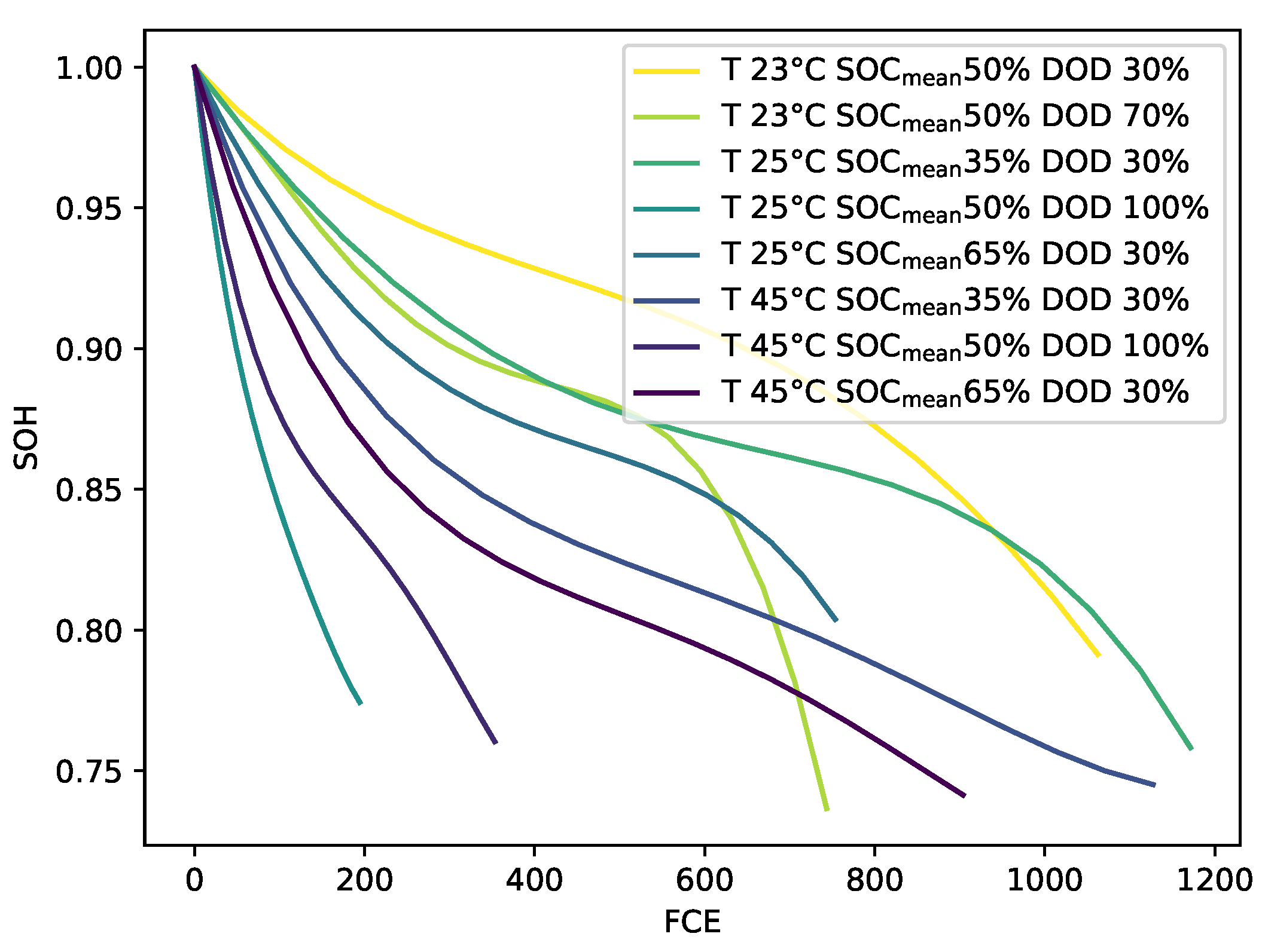
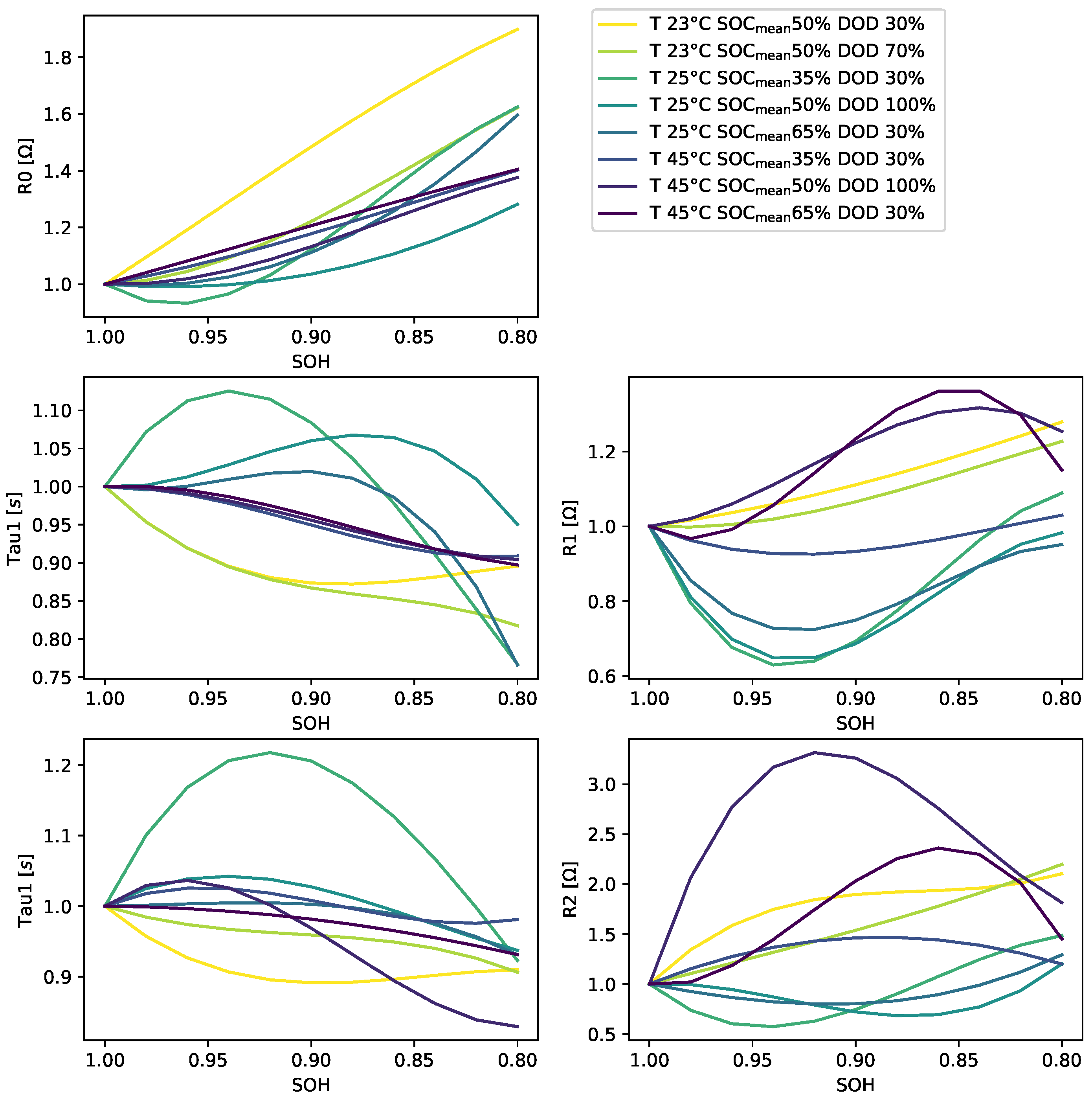
4.1. Ageing Data Processing

The fitting of the relaxations of each check-up leads to the identified dynamic parameters for various SOCs at different ageing states of each cell. For every stress factor combination, at least two cells were used. For every check-up, parameters for the charging and discharging directions are collected from the HPPC parts’ relaxations during the discharging and charging measurement of the incremental OCV. These datasets of each cell are combined as if it is one cell’s data. At first, the charging and discharging values of the parameters are combined and sampled to a fixed grid of SOCs. This is conducted in two steps. At first, the data are fitted using a fifth-degree polynomial. Then, the model is sampled with the original SOCs to be interpolated/extrapolated to the fixed grid of SOCs. The fit of a polynomial is helpful because the SOCs of the parameters in the charging and discharging directions differ, so by fitting a polynomial instead of calculating the mean, the step of bringing both to a fixed grid at this point is skipped, and a kind of trend line is estimated. The measurements represent the parameters for the charging and discharging directions and the colour changes with the SOC. However, a polynomial of a relatively high degree compared to the number of samples leads to problems resembling the behaviour outside the given SOCs. By combining the fit and the extrapolation, the estimate outside the given SOCs is more conservative. Another solution to the extrapolation can be the clipping of the characteristic map. Figure 9 shows an example of this process’s result.

A similar approach combines the capacities of the cells aged under the same stress factors over the full-cycle equivalents (FCEs). After combining the parameters for the charging and discharging directions, the parameters can be displayed as a 3D map over SOC and SOH. The following steps combine the maps of the different cells aged with the same stress factors, resulting in maps with a fixed SOC and SOH, which makes it easier for later usage. During this process, the maps of the group of battery cells are fitted using the lmfit package by defining a multidimensional polynomial. As before, this process eliminates the step of bringing all of the maps to the same fixed SOH values (see Figure 10).

At this point, the data of the cells that share the same stress factors are combined into a single dataset. The following steps include the design of the ageing model based on the data and how the degradation-based change is combined with the battery model.

4.2. Ageing Model

The ageing model, in general, is kept very simple. A simple way to implement a model is to create characteristic maps and access these maps with the extracted stress factors to obtain the parameters’ changes. The previously preprocessed data are further processed to obtain to the characteristic maps. For the characteristic map of the capacity, the data of the capacities are normalised to the first value of each dataset for each stress factor combination so that the graph corresponds to the SOH over the FCEs, as shown in Figure 11.

A similar approach is used for the other parameters, where at each ageing state the mean is calculated and normalised to its initial value. The parameters, consisting of RC resistances and time constants $\tau$ instead of the capacities, in addition to the battery cells’ internal resistance, do not follow a specific trend, see Figure 12. This is why the change in the other parameters is often neglected, and the modelling focuses on changing the internal resistance and the battery cell capacity.

These characteristic maps are used to calculate the parameters’ changes during degradation for the aggregated stress factors. These maps are combined with a simple method to extract the stress factors during runtime to calculate the change and add it to the change in the specific parameter. The feature extraction is performed by calculating the minimum and maximum SOC for the DOD and the mean temperature and by summing up the SOC and calculating the mean for a specified window based on the calculation of the FCE. The overall process of the ageing model consists of the continuous calculation of the FCE and stress factors that are fed into the characteristic map of the SOH over the FCE to obtain the change in SOH and the current SOH as follows:

$$\Delta SOH=SOH(SO{C}_{mean},T,DOD,FCE\left[k\right])-SOH(SO{C}_{mean},T,DOD,FCE[k-1])$$

(39)

$$SOH\left[k\right]=SOH[k-1]+\Delta SOH.$$

(40)

The calculated SOH[k] and the SOH[k − 1] of the last update are used to obtain the change in the dynamic parameters, P.

$$\Delta P=P(SO{C}_{mean},T,DOD,SOH\left[k\right])-P(SO{C}_{mean},T,DOD,SOH[k-1])$$

(41)

$$P\left[k\right]=P[k-1]+\Delta P.$$

(42)

By normalising the maps and calculating the change in the parameters, the battery model can be initialised with parameter maps that describe the behaviour of the parameters for different temperatures and SOCs. These initial maps are not normalised for the basic parameterisation. Therefore, the degradation of the parameters is included as a factor of the initial maps.

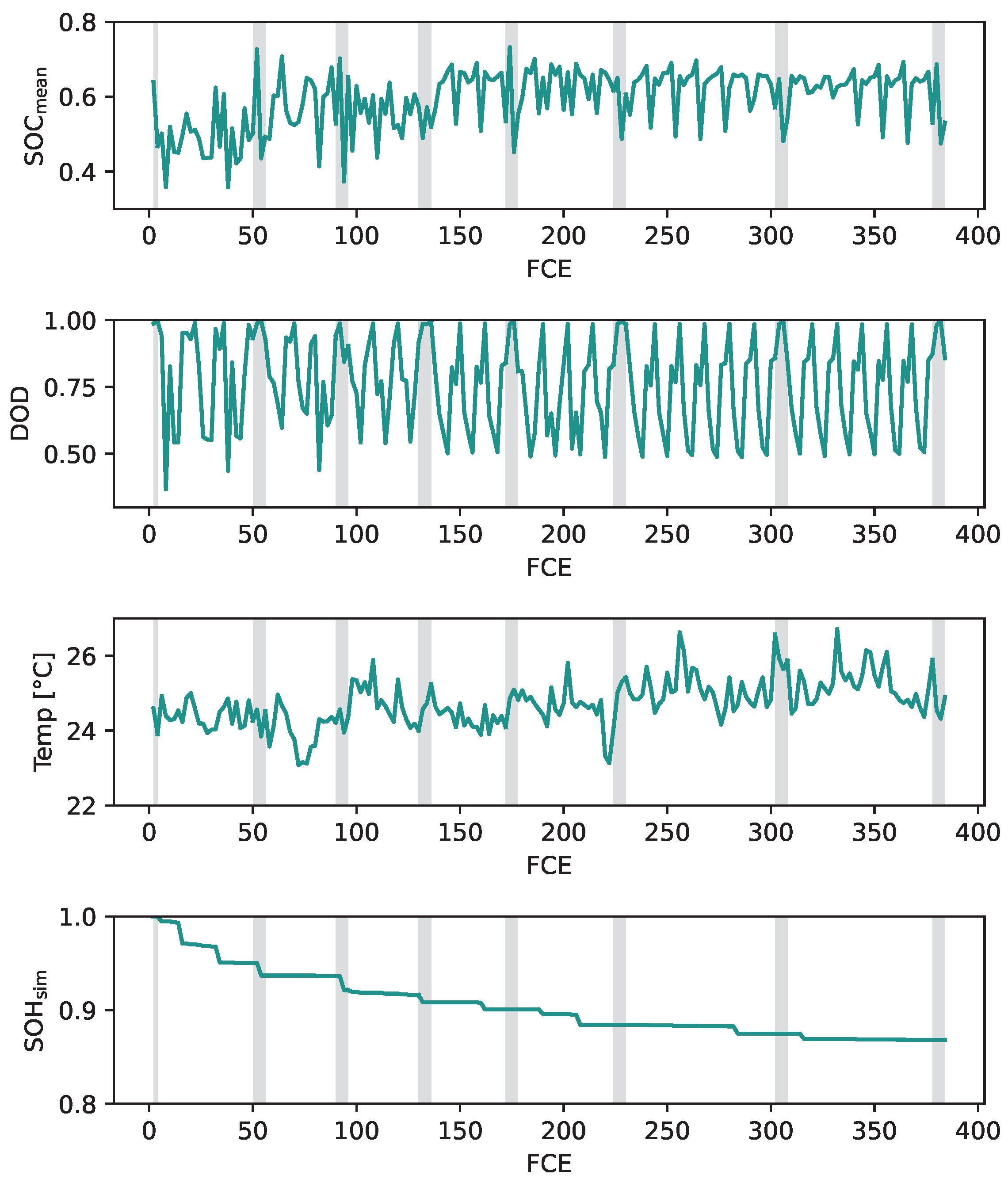
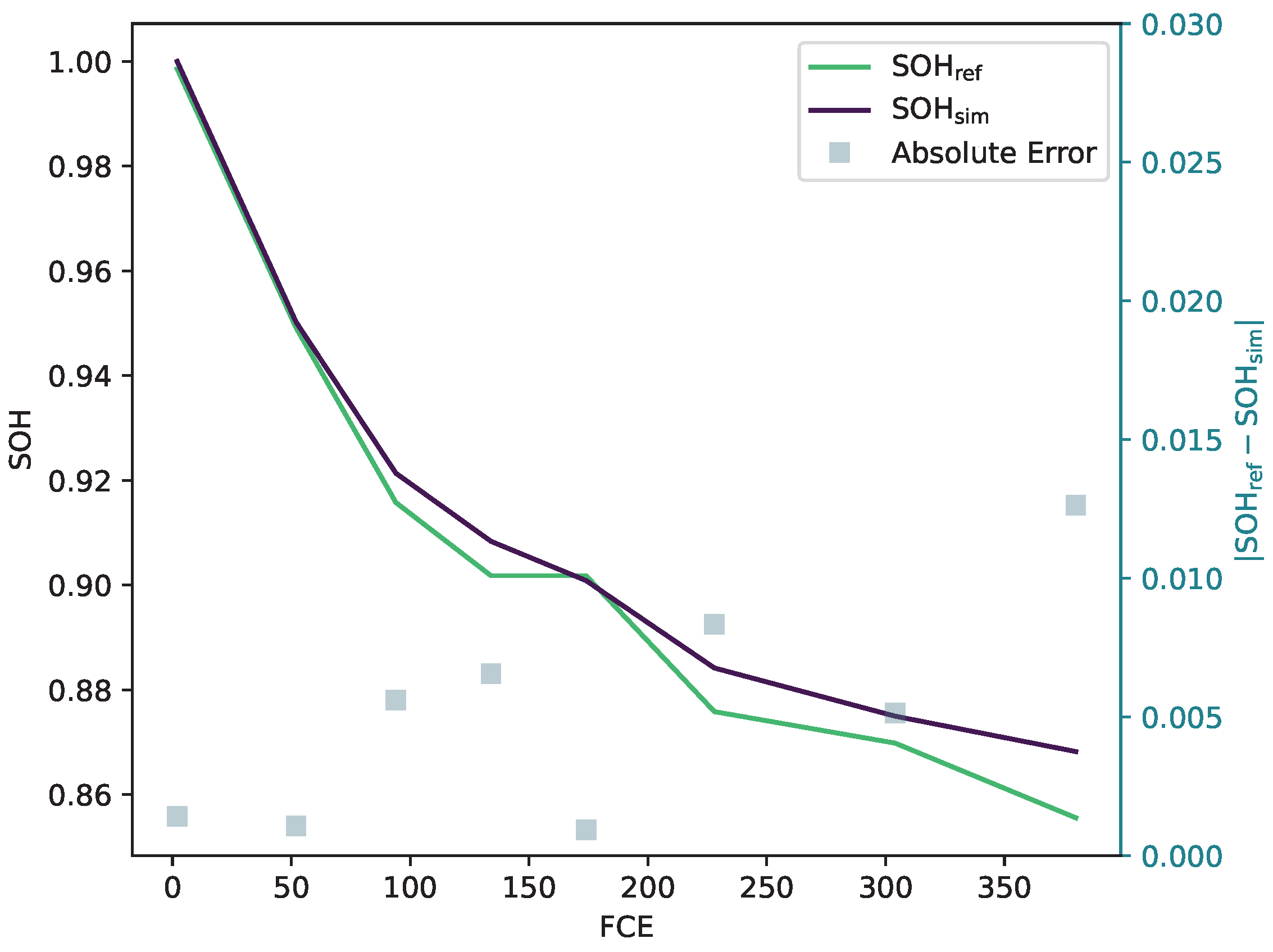
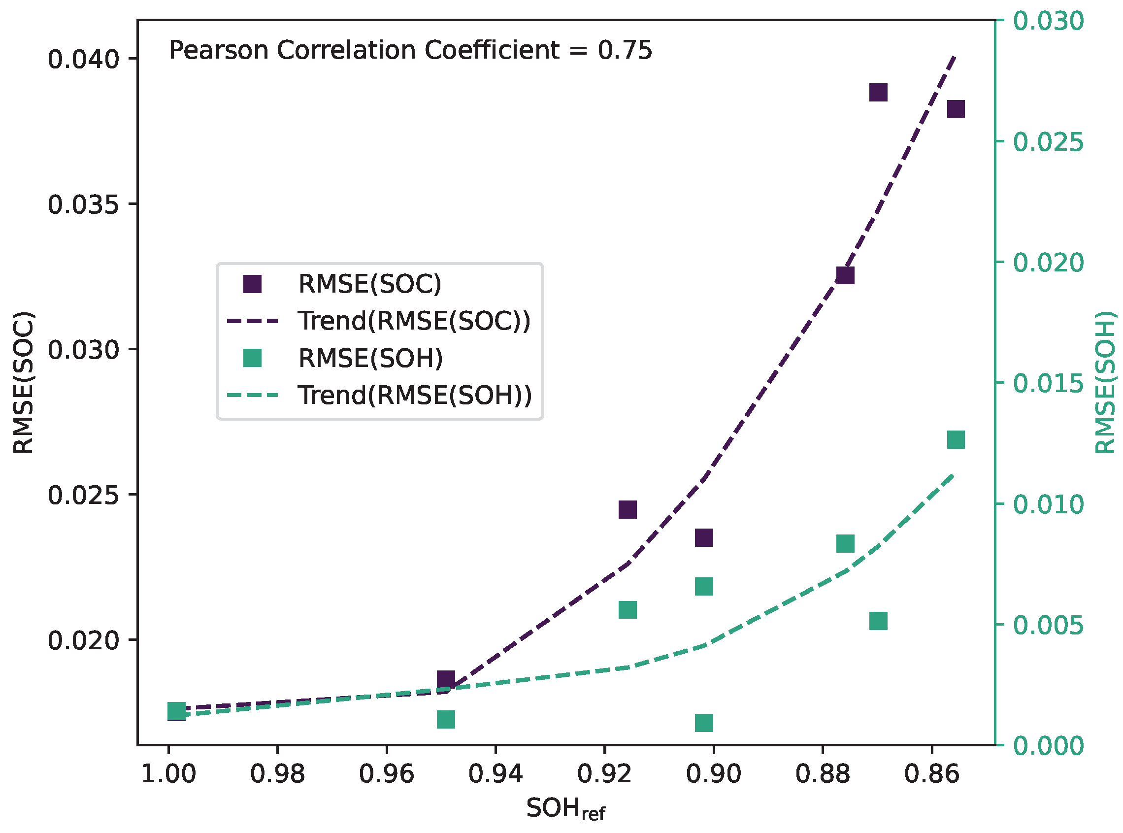
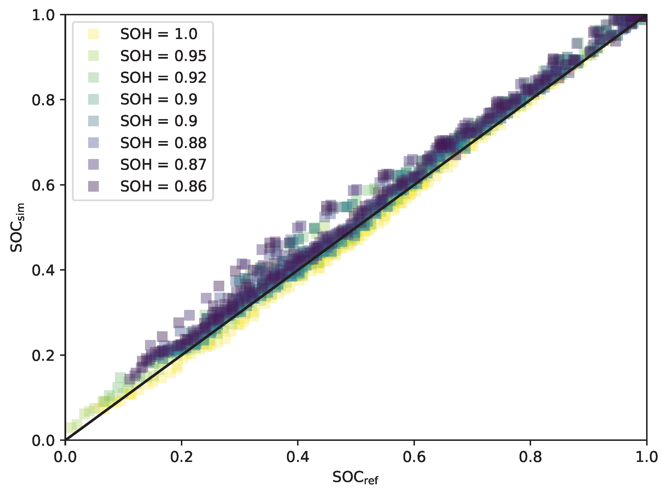
5. Results and Discussion

The validation of the whole system, consisting of implemented models and algorithms, is realised by iterating the data of the dynamically cycled cells. That means starting with the first check-up and alternating through check-up and cycling data. To do so without taking too much time, the data were resampled with a sampling rate of 1 $\mathrm{s}$ and the updating of the feature extractor was set to every two full-cycle equivalents. The extraction result is displayed in Figure 13.

The figure displays the degradation process of the battery cell. Check-ups are marked by a grey shaded area. During the degradation, the mean of the SOC is around 50% and transitions to about 65%, whereas the DOD switches between 50%, 80%, and full cycles. Smaller cycles are included, but since the feature extractor updates every two full-cycle equivalents the system is experiencing in this duration of bigger cycles, the small cycles are neglected. The temperature is, in general, about 25 °C and increases minimally during degradation. During the degradation process, the SOH estimation error increases over time. This is an expected behaviour since the ageing model does not represent dynamic ageing, and the feature extractor does not capture the stress factors of smaller stress cycles. The absolute error in the SOH rises to 1.2% at the end. The 1C capacity measured during the check-ups is used as a reference for the SOH. The evolution of the SOH in comparison to the reference and its absolute error is displayed in Figure 14.

The error in the ageing model is included in the SOC estimation since the model for the internal state prediction of UKF uses the capacity to calculate the current state vector, including the SOC. This circumstance leads to an increasing error in the SOC estimation of the degradation of the battery cell. Therefore, the SOC and SOH errors correlate as the Pearson correlation coefficient confirms, with a value of 0.75 (see Figure 15). The RMSE of the SOC is calculated for the dynamic sections of the check-ups because an SOC reference based on the measured capacity of the corresponding check-up can be used.

Interpreting the diagram leads to the conclusion that the error will rise faster with further degradation. It may then reach the limit of the implemented UKF. Nevertheless, the error in the SOC estimation is minimal, being about 4% at its maximum. A regression plot is generated to analyse the performance of the SOC estimation. The regression plot displays the performance of the estimated SOC (${\mathrm{SOC}}_{\mathrm{sim}}$) in contrast to the reference SOC (see Figure 16). When a marker is above the diagonal line, the SOC is overestimated. Otherwise, it is underestimated. The SOC was resampled for visibility reasons, only plotting every 300th estimate.

The diagram shows that during ageing, the SOC estimation is increasing, but especially in the range of the 20% to 60% SOC, the estimation has more outliers. Outliers might result from the change in the OCV during ageing, which is not part of the model because it was neglected during the system’s development. In addition to more outliers, the estimation overestimates the SOC with increasing degradation. This overestimation results from underestimating the degradation, leading to a higher SOH than the reference. Since the measurement segments start fully charged, the cell discharges slower than the reference suggests, resulting in the overestimation of the SOC.

Compared to other algorithms used in the literature, the system performs comparably to other implementations. In general, the RMSE lies in the range of about 1% to 2% SOC in the literature. The paper of Yang et al. [64] includes a survey for multiple approaches. However, the approaches are tested in simple circumstances where the cell is cycled with constant currents or schedules, such as the urban dynamic driving schedule that consists of multiple constant current pulses. They are sometimes tested on dynamic driving schedules such as the FUDS. They are only in rare cases validated on whole battery cell life and especially a cell life with dynamic profiles.

6. Conclusions

The results showed that the approaches combined in a system for the SOC and SOH estimation led to good results. The initial RMSE of the SOC is 1.75% and of the SOH is 0.0014%. It increases over the degradation to 3.82% for the SOC and 1.26% for the SOH. Therefore, the main problem is the evolution of the error over the cycling. There are multiple steps to improve the performance over the degradation. First, the feature extraction can be improved because it often labels a section with a non-dominant cycle. In addition, a new approach for the ageing estimation might be used, at least another model that does not rely on a look-up table. Furthermore, an approach to estimate the parameters online can be implemented to improve the estimate of the current capacity and, therefore, the SOC estimation over the degradation.

Overall the paper includes all the steps to set up an approach for SOC and SOH estimation with additions such as another discretisation of the model, an enhanced OCV sampling method, a specific parameterisation of the relaxation of the pulses, and a simple feature extraction. In contrast to the literature, this paper includes all the steps from measurements to modelling, parameterisation, ageing modelling, and bringing it together with feature extraction to run through a whole battery degradation process. The degradation consists of dynamic cyclic ageing and the check-ups in between, leading to the opportunity to analyse the influence of the SOH estimation on the SOC estimation and the performance of the approaches considering dynamic load profiles. By that, the introduced dataset and the displayed results are useful for testing algorithms over degradation and comparing them to the results.

References

1. Park, S.; Ahn, J.; Kang, T.; Park, S.; Kim, Y.; Cho, I.; Kim, J. Review of state-of-the-art battery state estimation technologies for battery management systems of stationary energy storage systems. J. Power Electron. 2020, 20, 1526–1540. [Google Scholar] [CrossRef]
2. Ungurean, L.; Cârstoiu, G.; Micea, M.V.; Groza, V. Battery state of health estimation: A structured review of models, methods and commercial devices. Int. J. Energy Res. 2017, 41, 151–181. [Google Scholar] [CrossRef]
3. Ali, M.U.; Zafar, A.; Nengroo, S.H.; Hussain, S.; Alvi, M.J.; Kim, H.-J. Towards a Smarter Battery Management System for Electric Vehicle Applications: A Critical Review of Lithium-Ion Battery State of Charge Estimation. Energies 2019, 12, 446. [Google Scholar] [CrossRef] [Green Version]
4. Kirchev, A. Battery Management and Battery Diagnostics. In Electrochemical Energy Storage for Renewable Sources and Grid Balancing; Elsevier: Amsterdam, The Netherlands, 2015; pp. 411–435. [Google Scholar]
5. Vezzini, A. Lithium-Ion Battery Management. In Lithium-Ion Batteries; Elsevier: Amsterdam, The Netherlands, 2014; pp. 345–360. [Google Scholar]
6. Wang, Y.; Tian, J.; Sun, Z.; Wang, L.; Xu, R.; Li, M.; Chen, Z. A comprehensive review of battery modeling and state estimation approaches for advanced battery management systems. Renew. Sustain. Energy Rev. 2020, 131, 110015. [Google Scholar] [CrossRef]
7. dos Reis, G.; Strange, C.; Yadav, M.; Li, S. Lithium-ion battery data and where to find it. Energy AI 2021, 5, 100081. [Google Scholar] [CrossRef]
8. Kollmeyer, P. Panasonic 18650PF Li-ion Battery Data. Mendeley Data 2018. [Google Scholar] [CrossRef]
9. Kollmeyer, P.; Vidal, C.; Naguib, M.; Skells, M. LG 18650HG2 Li-Ion Battery Data [Data Set]; Kaggle: San Francisco, CA, USA, 2023. [Google Scholar] [CrossRef]
10. De Craemer, K.; Trad, K. Cyclic Ageing with Driving Profile of a Lithium Ion Battery Module; Version 1; 4TU. ResearchData: Delft, The Netherlands, 2021. [Google Scholar] [CrossRef]
11. Jöst, D.; Ringbeck, F.; Blömeke, A.; Sauer, D.U. Timeseries Data of a Drive Cycle Aging Test of 28 High Energy NCA/C+Si Round Cells of Type 18650 = Zeitreihendaten eines Fahrzyklus-Alterungstests von 28 Hochenergie NCA/C+Si Rundzellen des Typs 18650; Institut für Stromrichtertechnik und Elektrische Antriebe: Aachen, Germany, 2021. [Google Scholar] [CrossRef]
12. Hu, X.; Feng, F.; Liu, K.; Zhang, L.; Xie, J.; Liu, B. State estimation for advanced battery management: Key challenges and future trends. Renew. Sustain. Energy Rev. 2019, 114, 109344. [Google Scholar] [CrossRef]
13. Ge, M.-F.; Liu, Y.; Jiang, X.; Liu, J. A review on state of health estimations and remaining useful life prognostics of lithium-ion batteries. Measurement 2021, 174, 109057. [Google Scholar] [CrossRef]
14. Berecibar, M.; Gandiaga, I.; Villarreal, I.; Omar, N.; van Mierlo, J. Critical review of state of health estimation methods of Li-ion batteries for real applications. Renew. Sustain. Energy Rev. 2016, 56, 572–587. [Google Scholar] [CrossRef]
15. Baghdadi, I.; Briat, O.; Delétage, J.-Y.; Gyan, P.; Vinassa, J.-M. Lithium battery aging model based on Dakin’s degradation approach. J. Power Sources 2016, 325, 273–285. [Google Scholar] [CrossRef]
16. Li, Y.; Liu, K.; Foley, A.M.; Zülke, A.; Berecibar, M.; Nanini-Maury, E.; Van Mierlo, J.; Hoster, H.E. Data-driven health estimation and lifetime prediction of lithium-ion batteries: A review. Renew. Sustain. Energy Rev. 2019, 113, 109254. [Google Scholar] [CrossRef]
17. Wang, Z.; Feng, G.; Zhen, D.; Gu, F.; Ball, A. A review on online state of charge and state of health estimation for lithium-ion batteries in electric vehicles. Energy Rep. 2021, 7, 5141–5161. [Google Scholar] [CrossRef]
18. Ling, L.; Wei, Y. State-of-Charge and State-of-Health Estimation for Lithium-Ion Batteries Based on Dual Fractional-Order Extended Kalman Filter and Online Parameter Identification. IEEE Access 2021, 9, 47588–47602. [Google Scholar] [CrossRef]
19. Bustos, R.; Gadsden, S.A.; Al-Shabi, M.; Mahmud, S. Lithium-Ion Battery Health Estimation Using an Adaptive Dual Interacting Model Algorithm for Electric Vehicles. Appl. Sci. 2023, 13, 1132. [Google Scholar] [CrossRef]
20. Du, C.-Q.; Shao, J.-B.; Wu, D.-M.; Ren, Z.; Wu, Z.-Y.; Ren, W.-Q. Research on Co-Estimation Algorithm of SOC and SOH for Lithium-Ion Batteries in Electric Vehicles. Electronics 2022, 11, 181. [Google Scholar] [CrossRef]
21. Gismero, A.; Schaltz, E.; Stroe, D.-I. Recursive State of Charge and State of Health Estimation Method for Lithium-Ion Batteries Based on Coulomb Counting and Open Circuit Voltage. Energies 2020, 13, 1811. [Google Scholar] [CrossRef] [Green Version]
22. Huang, Z.; Best, M.; Knowles, J.; Fly, A. Adaptive Piecewise Equivalent Circuit Model With SOC/SOH Estimation Based on Extended Kalman Filter. IEEE Trans. Energy Convers. 2023, 38, 959–970. [Google Scholar] [CrossRef]
23. Jin, S.; Yang, X.; Wang, C.; Wang, S.; Store, D.-I. A novel robust back propagation neural networkdual extended Kalman filter model for state-ofcharge and state-of-health co-estimation of lithiumion batteries. In Proceedings of the 2023 IEEE PES Conference on Innovative Smart Grid Technologies-Middle East (ISGT Middle East), Abu Dhabi, United Arab Emirates, 12–15 March 2023. [Google Scholar]
24. Lai, X.; Yuan, M.; Tang, X.; Yao, Y.; Weng, J.; Gao, F.; Ma, W.; Zheng, Y. Co-Estimation of State-of-Charge and State-of-Health for Lithium-Ion Batteries Considering Temperature and Ageing. Energies 2022, 15, 7416. [Google Scholar] [CrossRef]
25. Li, R.; Li, W.; Zhang, H. State of Health and Charge Estimation Based on Adaptive Boosting integrated with particle swarm optimization/support vector machine (AdaBoost-PSO-SVM) Model for Lithium-ion Batteries. Int. J. Electrochem. Sci. 2022, 17, 2. [Google Scholar] [CrossRef]
26. Li, Q.; Miao, S.; Liu, S.; Ma, B.; Qi, W.; Jin, W.; Cheng, Z. A Joint State Estimation Framework for Lithium-ion Batteries based on Hybrid Method. J. Phys. Conf. Ser. 2022, 2276, 12023. [Google Scholar] [CrossRef]
27. Liu, S.; Dong, X.; Yu, X.; Ren, X.; Zhang, J.; Zhu, R. A method for state of charge and state of health estimation of lithium-ion battery based on adaptive unscented Kalman filter. Energy Rep. 2022, 8, 426–436. [Google Scholar] [CrossRef]
28. Mahboubi, D.; Gavzan, I.J.; Saidi, M.H.; Ahmadi, N. State of charge estimation for lithium-ion batteries based on square root sigma point Kalman filter considering temperature variations. IET Electr. Syst. Transp. 2022, 12, 165–180. [Google Scholar] [CrossRef]
29. Ren, P.; Wang, S.; Huang, J.; Chen, X.; He, M.; Cao, W. Novel co-estimation strategy based on forgetting factor dual particle filter algorithm for the state of charge and state of health of the lithium-ion battery. Int. J. Energy Res. 2022, 46, 1094–1107. [Google Scholar] [CrossRef]
30. Xu, Y.; Chen, X.; Zhang, H.; Yang, F.; Tong, L.; Yang, Y.; Yan, D.; Yang, A.; Yu, M.; Liu, Z.; et al. Online identification of battery model parameters and joint state of charge and state of health estimation using dual particle filter algorithms. Int. J. Energy Res. 2022, 46, 19615–19652. [Google Scholar] [CrossRef]
31. Petzl, M.; Danzer, M.A. Advancements in OCV Measurement and Analysis for Lithium-Ion Batteries. IEEE Trans. Energy Convers. 2013, 28, 675. [Google Scholar] [CrossRef]
32. Kellner, Q.; Hosseinzadeh, E.; Chouchelamane, G.; Widanage, W.D.; Marco, J. Battery cycle life test development for high-performance electric vehicle applications. J. Energy Storage 2018, 15, 228. [Google Scholar] [CrossRef]
33. Klee Barillas, J.; Li, J.; Günther, C.; Danzer, M.A. A comparative study and validation of state estimation algorithms for Li-ion batteries in battery management systems. Appl. Energy 2015, 155, 455–462. [Google Scholar] [CrossRef]
34. Welch, G.; Bishop, G. An Introduction to Kalman Filter; University of North Carolina: Chapel Hill, NC, USA, 2006. [Google Scholar]
35. Ren, H.; Zhao, Y.; Chen, S.; Yang, L. A comparative study of lumped equivalent circuit models of a lithium battery for state of charge prediction. Int. J. Energy Res. 2019, 43, 7306–7315. [Google Scholar] [CrossRef]
36. Krewer, U.; Röder, F.; Harinath, E.; Braatz, R.D.; Bedürftig, B.; Findeisen, R. Review—Dynamic Models of Li-Ion Batteries for Diagnosis and Operation: A Review and Perspective. J. Electrochem. Soc. 2018, 165, A3656–A3673. [Google Scholar] [CrossRef]
37. Doyle, M.; Fuller, T.F.; Newman, J. Modeling of Galvanostatic Charge and Discharge of the Lithium/Polymer/Insertion Cell. J. Electrochem. Soc. 1993, 140, 1526–1533. [Google Scholar] [CrossRef]
38. Richardson, M.; Korotkin, I.; Ranom, R.; Castle, M.; Foster, J.M. Generalised single particle models for high-rate operation of graded lithium-ion electrodes: Systematic derivation and validation. Electrochim. Acta 2020, 339, 135862. [Google Scholar] [CrossRef] [Green Version]
39. Howey, D.A.; Bizeray, A.M.; Kim, J.-H.; Duncan, S.R. Parameterisation of the Single Particle Model for Lithium-Ion Cells. In Proceedings of the UKACC 12th International Conference on Control (CONTROL), Piscataway, NJ, USA, 5–7 September 2018. [Google Scholar]
40. Li, J.; Lotfi, N.; Landers, R.G.; Park, J. A Single Particle Model for Lithium-Ion Batteries with Electrolyte and Stress-Enhanced Diffusion Physics. J. Electrochem. Soc. 2017, 164, A874–A883. [Google Scholar] [CrossRef]
41. Pang, H.; Mou, L.; Guo, L.; Zhang, F. Parameter identification and systematic validation of an enhanced single-particle model with aging degradation physics for Li-ion batteries. Electrochim. Acta 2019, 307, 474–487. [Google Scholar] [CrossRef]
42. Lotfi, N.; Li, J.; Landers, R.G.; Park, J. Li-ion Battery State of Health Estimation based on an improved Single Particle model. In Proceedings of the American Control Conference, Seattle, WA, USA, 24–26 May 2017. [Google Scholar]
43. Laue, V.; Röder, F.; Krewer, U. Practical identifiability of electrochemical P2D models for lithium-ion batteries. Electrochim. Acta 2021, 51, 1253–1265. [Google Scholar] [CrossRef]
44. Moura, S.J.; Argomedo, F.B.; Klein, R.; Mirtabatabaei, A.; Krstic, M. Battery State Estimation for a Single Particle Model With Electrolyte Dynamics. IEEE Trans. Control Syst. Technol. 2017, 25, 453–468. [Google Scholar] [CrossRef]
45. Zhang, D.; Dey, S.; Couto, L.D.; Moura, S.J. Battery Adaptive Observer for a Single-Particle Model With Intercalation-Induced Stress. IEEE Trans. Control Syst. Technol. 2020, 28, 1363–1377. [Google Scholar] [CrossRef]
46. Saidani, F.; Hutter, F.X.; Scurtu, R.-G.; Braunwarth, W.; Burghartz, J.N. Lithium-ion battery models: A comparative study and a model-based powerline communication. Adv. Radio Sci. 2017, 15, 83–91. [Google Scholar] [CrossRef] [Green Version]
47. Lai, X.; Zheng, Y.; Sun, T. A comparative study of different equivalent circuit models for estimating state-of-charge of lithium-ion batteries. Electrochim. Acta 2018, 259, 566–577. [Google Scholar] [CrossRef]
48. Madani, S.S.; Schaltz, E.; Kær, S.K. A Review of Different Electric Equivalent Circuit Models and Parameter Identification Methods of Lithium-Ion Batteries. ECS Trans. 2018, 87, 23–37. [Google Scholar] [CrossRef]
49. Andrea, D. Lithium-Ion Batteries and Applications. A Practical and Comprehensive Guide to Lithium-Ion Batteries and Arrays, from Toys to Towns; Artech House: Boston, MA, USA, 2020. [Google Scholar]
50. Wu, J.; Jiao, C.; Chen, M.; Chen, J.; Zhang, Z. SOC Estimation of Li-ion Battery by Adaptive Dual Kalman Filter under Typical Working Conditions. In Proceedings of the 2019 IEEE 3rd International Electrical and Energy Conference (CIEEC), Beijing, China, 7–9 September 2019. [Google Scholar]
51. How, D.N.; Hannan, M.A.; Lipu, M.H.; Ker, P.J. A State of Charge Estimation for Lithium-Ion Batteries Using Model-Based and Data-Driven Methods: A Review. IEEE Access 2019, 7, 136116–136136. [Google Scholar] [CrossRef]
52. Fleischer, C.; Waag, W.; Heyn, H.-M.; Sauer, D.U. On-line adaptive battery impedance parameter and state estimation considering physical principles in reduced order equivalent circuit battery models part 2. Parameter and state estimation. J. Power Sources 2014, 262, 457–482. [Google Scholar] [CrossRef]
53. Sundaresan, S.; Devabattini, B.C.; Kumar, P.; Pattipati, K.R.; Balasingam, B. Tabular Open Circuit Voltage Modelling of Li-Ion Batteries for Robust SOC Estimation. Energies 2022, 15, 9142. [Google Scholar] [CrossRef]
54. Lavigne, L.; Sabatier, J.; Francisco, J.M.; Guillemard, F.; Noury, A. Lithium-ion Open Circuit Voltage (OCV) curve modelling and its ageing adjustment. J. Power Sources 2016, 324, 694. [Google Scholar] [CrossRef]
55. Yu, Q.-Q.; Xiong, R.; Wang, L.-Y.; Lin, C. A Comparative Study on Open Circuit Voltage Models for Lithium-ion Batteries. Chin. J. Mech. Eng. 2018, 31, 1–8. [Google Scholar] [CrossRef]
56. Pillai, P.; Kumar, P.; Pattipatti, K.R.; Balasingam, B. Open-Circuit Voltage Models for Battery Management Systems: A Review. Energies 2022, 15, 6803. [Google Scholar] [CrossRef]
57. Narula, M. Curve Curvature in Python. 2022. Available online: https://www.delftstack.com/howto/numpy/curvature-formula-numpy/ (accessed on 4 April 2023).
58. Wan, T.H.; Saccoccio, M.; Chen, C.; Ciucci, F. Influence of the discretization methods on the distribution of relaxation times deconvolution: Implementing radial basis functions with DRTtools. Electrochim. Acta 2015, 184, 483–499. [Google Scholar] [CrossRef]
59. Newville, M. Lmfit/lmfit-py: 1.1.0. Version: 1.1.0. Zenodo. 2022. Available online: https://lmfit.github.io/lmfit-py/ (accessed on 10 October 2022).
60. Brown, R.G.; Hwang, P.Y.C. Introduction to Random Signals and Applied Kalman Filtering: With MATLAB® Exercises; John Wiley and Sons, Inc.: Amsterdam, The Netherlands, 2012. [Google Scholar]
61. Haykin, S. Kalman Filtering and Neural Networks; John Wiley and Sons, Inc.: Amsterdam, The Netherlands, 2001. [Google Scholar]
62. Li, Y.; Vilathgamuwa, M.; Farrell, T.; Tran, N.T.; Teague, J. A physics-based distributed-parameter equivalent circuit model for lithium-ion batteries. Electrochim. Acta 2019, 299, 451–469. [Google Scholar] [CrossRef]
63. Goodfellow, I.; Bengio, Y.; Courville, A. Deep Learning; MIT Press: Cambridge, MA, USA, 2016. [Google Scholar]
64. Yang, B.; Wang, J.; Cao, P.; Zhu, T.; Shu, H.; Chen, J.; Zhang, J.; Zhu, J. Classification, summarization and perspectives on state-of-charge estimation of lithium-ion batteries used in electric vehicles: A critical comprehensive survey. J. Energy Storage 2021, 39, 102572. [Google Scholar] [CrossRef]
Figure 1. Schematic overview of the system depicting the UKF, the ageing model, and the feature extractor.
Batteries 09 00364 g001
Figure 2. Voltage diagram of check-up procedure, including capacity test, hybrid OCV and HPPC, and the validation.
Batteries 09 00364 g002
Figure 3. Voltage diagram of dynamic cycling procedure, including a capacity test.
Batteries 09 00364 g003
Figure 4. Steps of the Kalman filter.
Batteries 09 00364 g004
Figure 5. Electrochemical impedance spectra considering the sample time.
Batteries 09 00364 g005
Figure 6. Battery model with two RC elements.
Batteries 09 00364 g006
Figure 7. Sampling result of an OCV measurement.
Batteries 09 00364 g007
Figure 8. Result of the start parameter estimation and the fitting.
Batteries 09 00364 g008
Figure 9. Result of the combination of charging and discharging parameter values using fitting and extrapolation. Different colours of measurements represent the SOC value the parameter is estimated to have. The points belong to parameters estimated in the charging and discharging directions.
Batteries 09 00364 g009
Figure 10. Result of the combination of different cells using a multidimensional polynomial fit.
Batteries 09 00364 g010
Figure 11. Resulting characteristic map for the capacities.
Batteries 09 00364 g011
Figure 12. Resulting characteristic map for the dynamic parameters.
Batteries 09 00364 g012
Figure 13. Features extracted over laboratory battery life. Check-ups are marked by a grey shaded area.
Batteries 09 00364 g013
Figure 14. Comparison of the estimated SOH and the reference SOH.
Batteries 09 00364 g014
Figure 15. RMSE of the estimated SOC and SOH with their trendline and Pearson correlation coefficient.
Batteries 09 00364 g015
Figure 16. Regression plot of the SOC for different ageing states.
Batteries 09 00364 g016