Genetic Algorithm and Taguchi Method: An Approach for Better Li-Ion Cell Model Parameter Identification

Abstract

The genetic algorithm (GA) is one of the most used methods to identify the parameters of Li-ion battery models. However, the parametrization of the GA method is not straightforward and can lead to poor accuracy and/or long calculation times. The Taguchi design method provides an approach to optimize GA parameters, achieving a good balance between accuracy and calculation time. The Taguchi design method is thus used to define the most adapted GA parameters to identify the parameters of model of Li-ion batteries for household applications based on static and dynamic tests in the time domain. The results show a good compromise between calculation time and accuracy (RMSE less than 0.6). This promising approach could be applied to other Li-ion battery applications, resulting from measurements in the frequency domain or different kinds of energy storage.

1. Introduction

Lithium-ion batteries used in electric vehicles (EVs) degrade significantly in the first five years of operation and are designed for a useful life of about eight years, equivalent to a twenty percent loss in initial capacity [1]. Nevertheless, even if they no longer meet EV performance standards, these batteries are still capable enough to serve less demanding applications, including stationary energy-storage services [2], lowering storage system prices and leading to a potential solar energy revolution [3,4,5]. Indeed, it is estimated that by 2030, stationary storage powered by used EV lithium-ion batteries could exceed 5 GWh [6]. However, few studies on second-life EV batteries have been published in terms of assessing the technical feasibility, economic viability and, in the positive case, a protocol of use to maximize their second-life usage in solar storage systems [1]. Any attempt to do so requires validating a digital twin, which we tried to achieve in this paper.

Battery modeling approaches can be summed up into three approaches: the electrochemical or physics-based model; the black-box model; and the equivalent electric circuit model (EECM) [7]. However, the latter is the most widely used model in battery management systems (BMS) due to its simplicity and reasonable accuracy [8]. In addition, EEC models are highly recommended for observation and control problems and could be considered a solid foundation for state-of-charge (SOC) and state-of-health (SOH) estimations in low dynamic applications.

In [9,10], the authors compared the performance between 1-RC, 2-RC, and 3-RC EEC models. They used electrochemical impedance spectroscopy to derive 26.9 V Li-ion battery pack impedances at different SOC points. The impedances versus SOC relationships were considered third-degree polynomials, and the coefficients were fitted using the MATLAB genetic algorithm solver. The proposed models were then validated by two different real-world driving cycles reproduced by a hardware-in-the-loop platform. The 3-RC EECM scored the best root mean square error (RMSE) with a value of less than 0.6%. This paper uses a third-order EECM to reproduce Li-ion cell behavior. A C/40 rate (dis)charging test was conducted to obtain the open circuit voltage (OCV) versus SOC relationship and a dynamic profile extracted from a real-world solar application for parameter fitting and validation. Usually, the GA is used with default parameters [9,11], with a set of predefined parameters [12], or using the trial-and-error method, which may not be suitable for the application under study and may take a long time without obtaining the desired solution. In contrast to the previously mentioned studies, the RC differential equations with constant parameters are used to describe the cell dynamics, and the hysteresis effect was considered. For parameter identification, the genetic algorithm solver in MATLAB, combined with a systematic approach based on the Taguchi experimental design and ANOVA (analysis of variance), is implemented. The RMSE of the model obtained is also less than 0.6%, with accuracy reaching more than 99.44%.

The novelty and contribution of this study can be summarized as follows:

• Provide an easy-to-implement, robust, and systematic approach to the characterization of a Li-ion cell from experimentation, to modeling, to validation.
• The parameters used for setting the GA have been justified using the Taguchi method and proven to make the algorithm more efficient in terms of computation time and model fitting.
• The GA parameter optimization method could be generalized and used for other characterization techniques (e.g., particle swarm optimization).
• A real-word household power consumption profile was used to parametrize the cell model; therefore, this study is a solid basis for further investigation on the use of second-life Li-ion batteries in solar home storage systems.

This paper is organized as follows. Section 2 describes the series of laboratory tests conducted to parametrize the lithium-ion cell model. In Section 3, the cell EECM is described. Section 4 elaborates on the parameter identification approach, followed by Section 5 which shows a set of estimated cell voltages versus measured cell voltages. Finally, Section 6 concludes the paper.

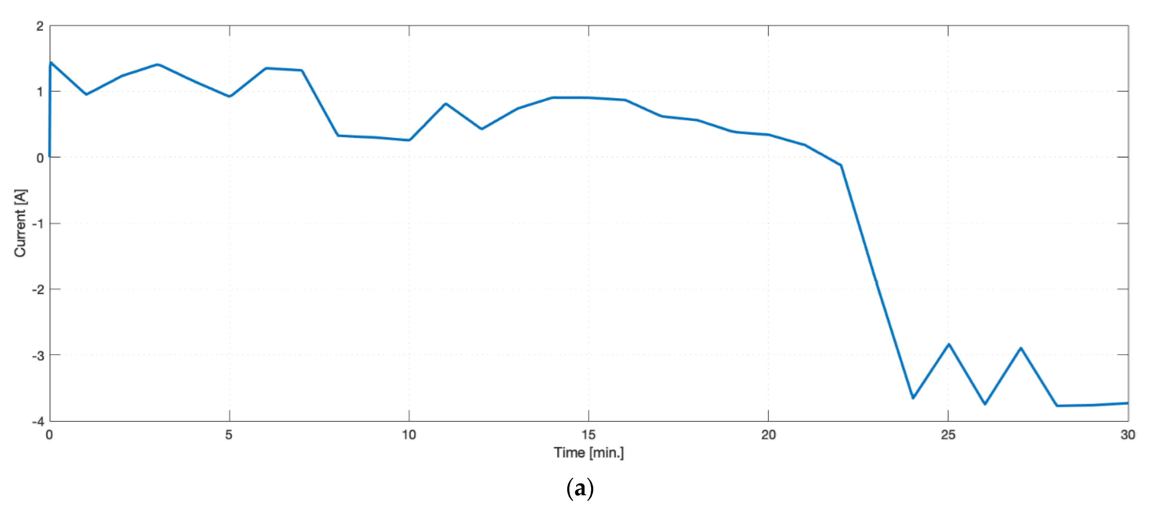
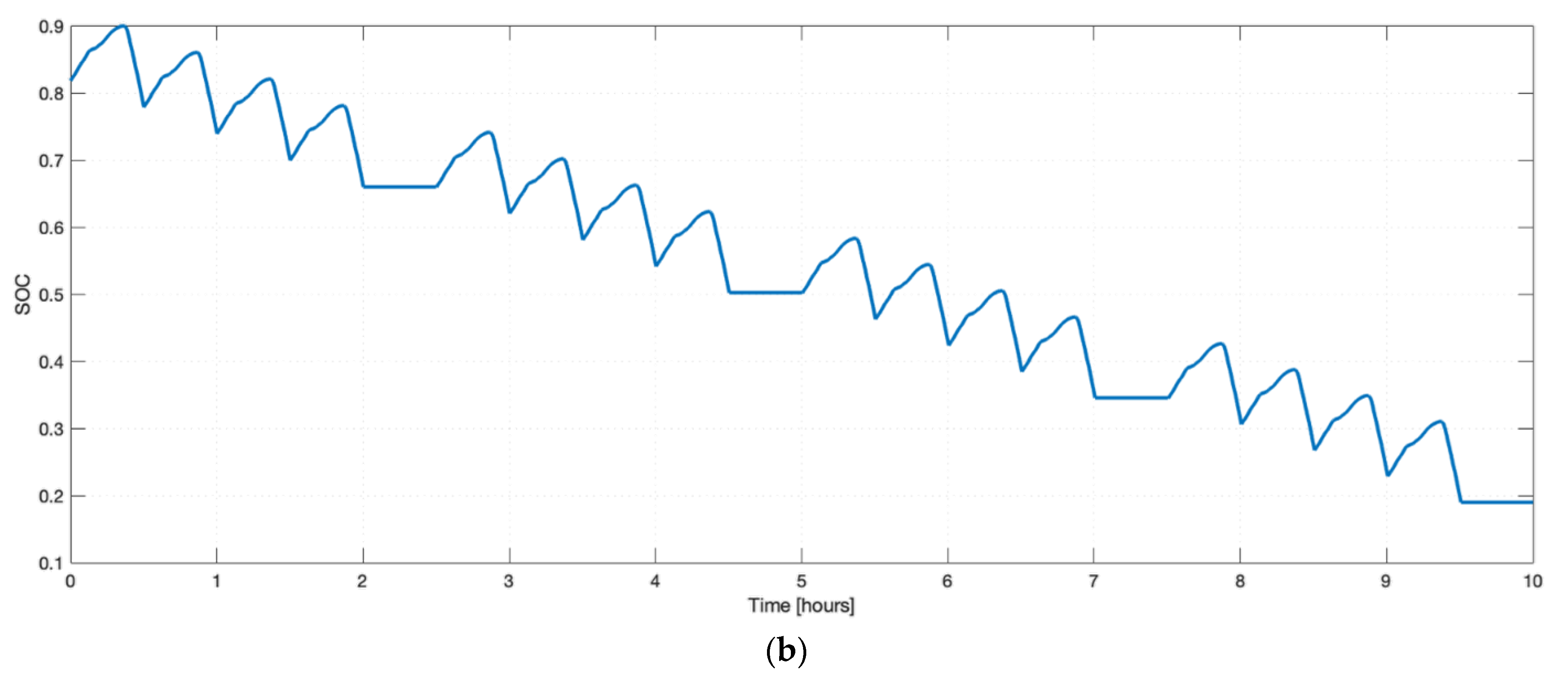
2. Brief Introduction of Collected Dataset

The experiments were conducted using two INR 18650 MJ1 Li-ion cells. Data were collected from the first cell to fit the parameter values to the ECCM and from the second cell to validate the model. These cells comprise nickel-rich NMC811 cathodes and graphite-silicon anodes with a nominal capacity of 3.5 Ah and a nominal voltage of 3.6 V, which can be used across a wide range of applications from spacesuits to automotive vehicles [13]. In addition, the test bench includes a battery-regenerative test system for the charge, discharge, and measurements; a thermal chamber for thermal conditioning; and a computer for data monitoring and control. During the tests, the thermal and electrical variables were measured and registered with an acquisition time from 1 to 60 s, depending on the different steps of the test. Therefore, the frequency value was conveniently chosen for each step to record all the significant changes and simultaneously save the length of the data files.

Electric consumption data are indispensable to facilitating the employment of decentralized renewables [14]. It helps engineers and researchers size renewable sources, manage and optimize the energy flow, and reduce costs. There are roughly three techniques used to generate a load profile [15]. First, the top-down model, or the measurement-based approach, uses routinely acquired data from measuring devices placed at different locations in the system. Hence, the quality of real-time-collected data heavily depends on the sensors’ accuracy. Moreover, the top-down model requires a minimum of six months of historical data, as long as it includes both summer and winter, to generate or forecast a functional load profile. Second, the bottom-up model, or the component-based approach, requires the energy consumed by each electrical appliance to be obtainable. For this, two methods are adopted. In the first one, all the components are metered, and no historical data are required. However, this process is time and money-consuming. In the second one, none or part of the components are metered, and the energy consumed by the rest is estimated. Finally, the hybrid model, which combines the two techniques mentioned previously, benefits from the low cost of the top-down approach and the excellent theoretical accuracy of the bottom-up approach [16]. A French household power consumption dataset [17] collected between December 2006 and November 2010 in a house in Seaux using the top-down approach was used as a reference for our work. It provides 2,075,259 measurements of global active power with a one-minute step-time. This dataset accompanies no reference paper; however, it has been used by [18] to quantify self-consumption linked to solar home battery systems and by [19] to forecast power consumption using machine-learning algorithms.

Three tests were performed. The first test evaluated the OCV versus SOC relationship at 25 °C. It consists of fully discharging the cell, charging the cell at a C/40 rate until fully charged, and discharging at a C/40 rate until fully discharged. Two voltage versus SOC relationships for the charge and discharge portion of the test were derived from the test data. The OCV (SOC, 25°) was computed as the average. Indeed, (dis)charging the battery at a low rate pares the ohmic and polarization effects so that the cell can be considered at equilibrium at each point in time [20,21,22].

The cell starts at about 80% SOC in the second test (Figure 1), followed by 16 current waveform cycles. Every four cycles are separated by a 30 min rest, and each cycle is equivalent to about a 3.9% SOC decrease. The current waveform was computed by subtracting the power consumed by the French household mentioned above from the power generated by a 3.6 kW PV installation during 30 min of 1 January 2008 in Seaux, France, and normalized from a 48 V 2 kWh Li-ion pack level to a cell level. Indeed, the EECM parameter values are significantly affected by the final application as well as the cell SOC [9]. Therefore, the profile used should be representative of the chosen application and applied across the whole SOC operation range to find the optimal parameter combination for the entire range.

Finally, in the third test, the second cell underwent four cycles from the current waveform mentioned above, and the data collected were used to validate the model.

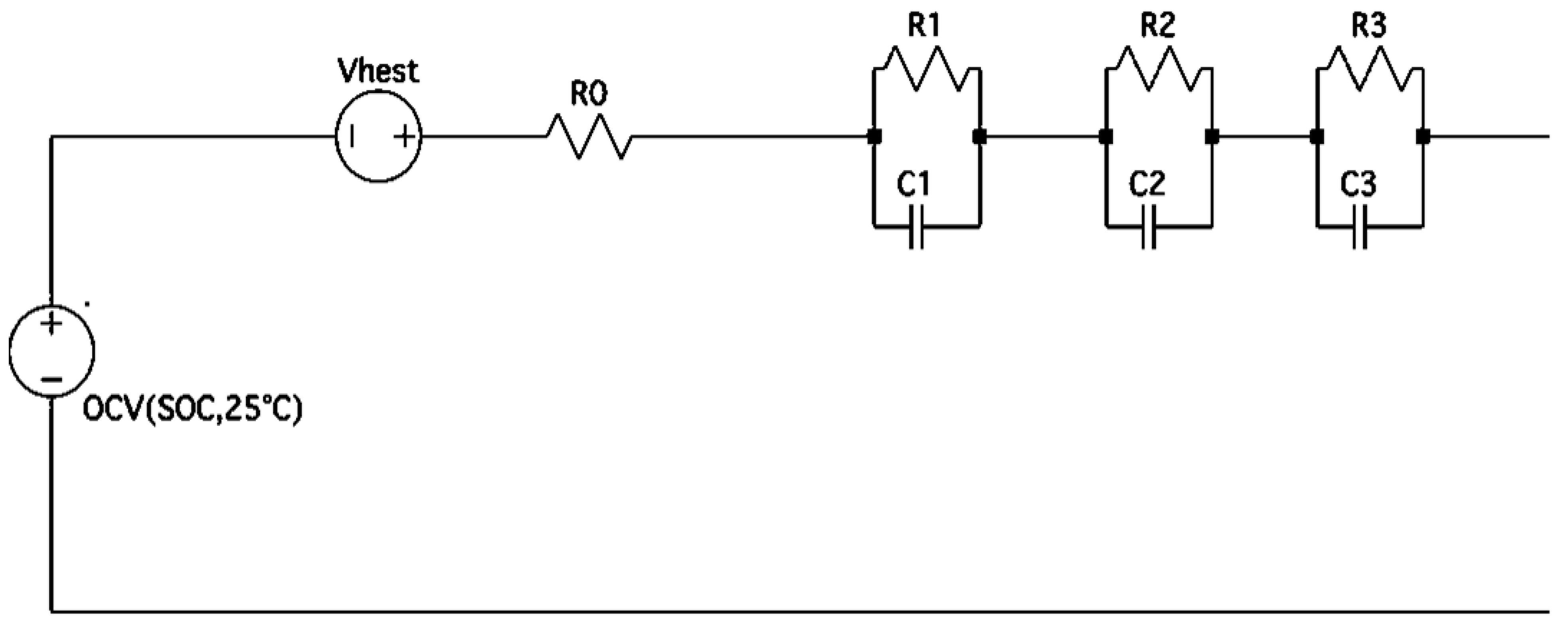
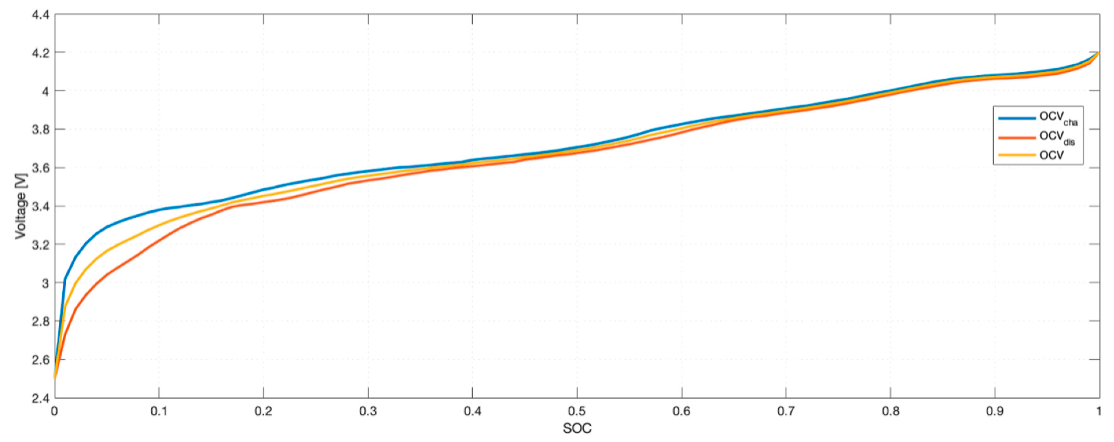
3. Lithium-Ion Cell Modelling

The EEC models describe the battery’s electrical behavior in terms of voltages and currents. Using only passive electrical components, the resulting equations are a low-dimensional system of ordinary differential equations, which are generally nonlinear because the battery parameter depends on the temperature and the state of charge. To reduce the complexity further, only the open circuit voltage is assumed to have dependencies on temperature and state of charge. Therefore, it is estimated at multiple states of charge points and temperatures via laboratory tests, and then interpolated to deduce the continuous OCV–SOC relationships. As a result, these models are relatively accurate and less complex, making them a competitive candidate to be embedded in battery management systems for real-life applications, ensuring reliable and safe operating conditions.

In this section, the third-order EECM is introduced. As shown in Figure 2, the model used in [9] has been modified by adding the hysteresis effect and by using electrical-circuit differential equations to imitate dynamic cell behavior instead of parameters versus SOC polynomial relationships.

The cell OCV and SOC are highly correlated and can be significantly influenced by temperature [23]. It is usually measured by applying current pulses with known SOC alternations, letting the battery rest for at least 30 min before finally measuring the terminal voltage [11]. However, the static test adopted in this paper consists of (dis)charging at a prolonged rate (i.e., C/40), owing to its high SOC resolution and ease of implementation (Figure 3).

The observed instantaneous voltage variation when charging or discharging the cell is modeled by an ohm internal resistance [24]. The multiple series RC branches in the EECM emit the voltage dynamic deviation from the OCV when the cell undergoes an input current and slow recovery when the cell is allowed to rest. This is usually referred to as the polarization effect [25], which is caused by the slow migration of lithium in the cell [9].

Figure 4 shows that averaging the two voltage versus SOC relationships obtained considerably decreases the hysteresis effect. However, [26] showed that a 1% battery’s OCV measurement noise is equivalent to a 29.8% error increase in SOC estimation. Therefore, the Plett single-state hysteresis model was considered in this study [22]:

$$V_{hest}\left(t\right)=M.h\left(t\right)+M_0.sgn\left(i\left(t\right)\right)$$

(1)

where M₀.sgn(i(t)) models the instantaneous hysteresis when the input current sign changes, and M.h(t) models the dynamic hysteresis when the SOC cell changes. h(t) is a normalized hysteresis contribution between +1 and −1, and M the maximum polarization voltage due to hysteresis. The derivative of h(t) can be expressed as:

$$\dot{h}\left(t\right)=-\left|\eta \left(t\right).i\left(t\right).\gamma \left(t\right)/Q\right|.\left(sgn\left(i\left(t\right)\right)+h\left(t\right)\right)$$

(2)

where $\gamma$(t) is the rate of the hysteresis decay toward either +1 or −1.

The cell model state-space representation can be expressed as follow:

$$\left[\begin{array}{c}\dot{SOC}\left(t\right)\\ \begin{array}{c}\dot{h}\left(t\right)\\ {\dot{V}}_1\left(t\right)\\ {\dot{V}}_2\left(t\right)\end{array}\\ {\dot{V}}_3\left(t\right)\end{array}\right]=\left[\begin{array}{ccccc}1& 0& 0& 0& 0\\ 0& -\left|\frac{\eta \left(t\right).i\left(t\right).\gamma \left(t\right)}{Q}\right| & 0& 0& 0\\ 0& 0& -\frac{1}{{\tau }_1}& 0& 0\\ 0& 0& 0& -\frac{1}{{\tau }_2}& 0\\ 0& 0& 0& 0& -\frac{1}{{\tau }_3}\end{array}\right]\left[\begin{array}{c}SOC\left(t\right) \\ \begin{array}{c}h\left(t\right)\\ V_{C_1}\left(t\right)\\ V_{C_2}\left(t\right)\end{array}\\ V_{C_3}\left(t\right)\end{array}\right]+\left[\begin{array}{cc}\frac{-1}{Q}\eta & 0\\ 0& -\left|\frac{\eta \left(t\right).i\left(t\right).\gamma \left(t\right)}{Q}\right|\\ \frac{1}{C_1}& 0\\ \frac{1}{C_2}& 0\\ \frac{1}{C_3}& 0\end{array}\right]\left[\begin{array}{c}i\left(t\right)\\ sgn\left(i\left(t\right)\right)\end{array}\right]$$

(3)

$$V\left(t\right)=\left[\begin{array}{ccccc}1& -M& 1& 1& 1\end{array}\right]\left[\begin{array}{c}OCV\left(t\right)\\ \begin{array}{c}h\left(t\right)\\ V_{C_1}\left(t\right)\\ V_{C_2}\left(t\right)\\ V_{C_3}\left(t\right)\end{array}\end{array}\right]+\left[\begin{array}{cc}{R}_0& -M_0\end{array}\right]\left[\begin{array}{c}i\left(t\right)\\ sgn\left(i\left(t\right)\right)\end{array}\right]$$

(4)

where the OCV can be interpolated from the OCV versus SOC relationship, $\eta$ is the coulombic efficiency, Q the total capacity, and ${\tau }_k$ the k-RC time constant. It should be noted that, regarding the sign convention, i(t) is positive when charging and negative when discharging.

4. EECM Parameter Identification Approach

4.1. Genetic Algorithm

Genetic algorithms (GAs) are stochastic optimization and global search methods that imitate natural biological evolution [27]. A GA operates on a population of artificial individuals. A chromosome represents each individual, and each chromosome expresses a solution to a problem and has a fitness (i.e., a number that measures how good a solution is to the given problem). Starting with a randomly generated population of individuals, a GA carries out a survival of the fittest-based selection and the recombination process to derive the next generation’s successor population. During recombination, parent chromosomes are selected, and their genetic material is recombined to produce child chromosomes. However, the offspring generated using the selected parents only have the characteristics of its parents, including their drawbacks. Therefore, random mutations must be applied to each offspring to overcome the problem and create new individuals, preventing the evolution from freezing. As in natural adaptation, this process leads to the evolution of individuals more suitably adapted to their environment than the individuals from which they were derived until some stopping criterion is reached.

The GAs lifecycle can be summarized as follow:

• Create a population of random chromosomes (potential solutions);
• Score each chromosome in the population for fitness, and ‘usually’ select individuals with better fitness values as parents;
• Create a new generation through crossover and mutation;
• Repeat until some criteria is reached (e.g., max number of generations, max amount of time running);
• Emit the fittest chromosome as the solution.

4.2. Systematic Approach Based on Taguchi Experimental Design

The GA is a well-proven solution for complicated estimation problems [12] due to its numerous advantages, notably its capability to usually converge despite how far the initial conditions are from the optimal solution and how many unknown variables are used as long as they are bounded. However, it can be time-consuming to run and can sometimes be stuck in local minima. The authors of [28] showed that optimizing the GA solver parameters can overcome these limitations. Therefore, they proposed a systematic and comprehensible approach based on the Taguchi experimental design for parameter tuning, which will be replicated in this paper while considering only the parameters levels suitable in our case (

Table 1. Solver options and their experimental levels.

No.	Parameters	Code	Level
			1	2	3
1	Migration Direction	A	Forward	Both	-
2	Population Size	B	100	150	200
3	Fitness Scaling Function	C	Proportional	Rank	Top
4	Selection Function	D	Remainder	Tournament	Roulette
5	Elite Count	E	1	5	10
6	Crossover Fraction	F	0.3	0.7	0.9
9	Crossover Function	G	Two Point	Scattered	Arithmetic
8	Mutation Function	H	Adaptive xsqFeasible	Uniform	Gaussian

).

4.2.1. Generating Taguchi Experimental Design

The experimental design proposed by Taguchi involves orthogonal arrays to organize the parameters affecting the GA solver and the levels at which they should be varied. Instead of testing all possible combinations, the Taguchi method tests pairs of combinations, gathering the necessary data to determine which factors most affect the GA solver with minimum experimentation [29]. As presented in Table 1, we had one GA parameter with two levels, and the rest had three levels. The Taguchi orthogonal array design L18 (2¹ 3⁷) was chosen and generated by Minitab (

Table 2. Taguchi Orthogonal Array design L18 (2¹ 3⁷).

Experiment	Parameters of ga Solver
	A	B	C	D	E	F	G	H
1	1	1	1	1	1	1	1	1
2	1	1	2	2	2	2	2	2
3	1	1	3	3	3	3	3	3
4	1	2	1	1	2	2	3	3
5	1	2	2	2	3	3	1	1
6	1	2	3	3	1	1	2	2
7	1	3	1	2	1	3	2	3
8	1	3	2	3	2	1	3	1
9	1	3	3	1	3	2	1	2
10	2	1	1	3	3	2	2	1
11	2	1	2	1	1	3	3	2
12	2	1	3	2	2	1	1	3
13	2	2	1	2	3	1	3	2
14	2	2	2	3	1	2	1	3
15	2	2	3	1	2	3	2	1
16	2	3	1	3	2	3	1	2
17	2	3	2	1	3	1	2	3
18	2	3	3	2	1	2	3	1

).

4.2.2. Conducting the Experiments

In [28], the authors considered fixing the computation time for every experiment, seeking a fair comparison. However, time can be seen as a ‘factor’ in extensive data and parameter numbers; therefore, fixing it can degrade the statistical analysis of GA solver options’ contribution. In this paper, the computation time of every experiment was fixed to 30 s. However, from the significance analysis, it was expected that the set of GA parameters contribute to minimizing the computation time, while being convergent to a reasonable fitness value.

The cost function chosen was the root mean square error (RMSE):

$$RMSE=\sqrt{\frac{1}{N}{\sum }_i^N{\left({\breve{V}}_i-{\widehat{V}}_i\right)}^2}$$

(5)

where ${\check{V}}_i$ is the cell measured voltage, and ${\widehat{V}}_i$ is the cell estimated voltage.

The GA solver parameters set according to the Taguchi array are shown in Table 2, and the simulation procedure is summarized in Figure 5. For consistency, every experiment was repeated three times as shown in

Table 3. Experimental layout and data.

Experiment	Parameters of ga Solver								RMSE %
	A	B	C	D	E	F	G	H	Run 1	Run 2	Run 3
1	1	1	1	1	1	1	1	1	0.945	0.812	0.797
2	1	1	2	2	2	2	2	2	0.615	0.784	0.698
3	1	1	3	3	3	3	3	3	1.410	1.841	0.816
4	1	2	1	1	2	2	3	3	0.989	1.162	1.526
5	1	2	2	2	3	3	1	1	0.706	0.752	0.674
6	1	2	3	3	1	1	2	2	0.699	0.715	0.650
7	1	3	1	2	1	3	2	3	0.744	0.889	0.829
8	1	3	2	3	2	1	3	1	0.793	2.161	1.265
9	1	3	3	1	3	2	1	2	0.634	0.665	0.621
10	2	1	1	3	3	2	2	1	0.642	0.675	0.842
11	2	1	2	1	1	3	3	2	1.131	1.022	0.990
12	2	1	3	2	2	1	1	3	0.632	0.811	0.7889
13	2	2	1	2	3	1	3	2	0.791	0.944	0.800
14	2	2	2	3	1	2	1	3	0.657	0.905	0.614
15	2	2	3	1	2	3	2	1	0.642	0.636	0.6390
16	2	3	1	3	2	3	1	2	0.766	0.703	0.7802
17	2	3	2	1	3	1	2	3	0.978	1.109	0.917
18	2	3	3	2	1	2	3	1	1.456	1.890	0.891

.

4.2.3. Analyzing Data

ANOVA was used at a 95% confidence level to determine the effect and contribution of each parameter on the experiment outcome. The ‘Cross-over Function’ p-value in

Table 4. ANOVA analysis.

Source	DF	Adj SS	Adj MS	F	p
A	1	0.06578	0.06578	0.92	0.381
B	2	0.18040	0.18040	2.53	0.173
C	2	0.23933	0.11966	1.68	0.277
D	2	0.21353	0.10677	1.50	0.309
E	2	0.00555	0.00555	0.08	0.791
F	2	0.04346	0.04346	0.61	0.470
G	2	2.04866	1.02433	14.36	0.008
H	2	0.44251	0.22125	3.10	0.133
Error	2	0.35666	0.07133
Total	17	3.59588

, which is less than 0.005 [30], indicates that it significantly contributed to rapidly converging towards a reasonable optimal RMSE, in the ideal case. Its level was chosen from the effect charts (Figure 6) to ensure rapid convergence, minimizing the computation time, and the non-significant factors from the experiments delivered the best fitness value (

Table 5. Selected solver option set.

A	B	C	D	E	F	G	H
Both	150	Proportional	Remainder	10	0.9	Two Point	Uniform

).

5. Results and Discussion

To test the developed Li-ion EECM and the proposed GA parameter optimization, a dynamic profile extracted from a real-world solar application was used. Figure 7 shows the results for cell I from which the laboratory data were collected to identify the model parameters. The estimated versus measured voltage was fairly accurate across each input current cycle. The RMSE error of the model was 0.59% with a maximum error rate of 0.6% (Figure 8), giving an accuracy of 99.4%, which is comparable with the results obtained by [9]. Figure 9 gives a zoomed-in view of the transient shape, which smoothly follows the measured voltage.

To validate the model, laboratory data were collected from another cell of the same type. Figure 10 and Figure 11 show that the model was also accurate, with an accuracy of more than 99.4%.

The estimation results show that the developed model can reflect the dynamic of the lithium-ion cell and can also be used at a pack level. However, improvements can be made regarding the use of the cell for a more extended SOC range; a new set of the EECM parameters should be identified for this specific range. It should be noted that the EECM can be classified as an empirical model; therefore, even a high-order EECM cannot provide itself any insight into internal dynamics and, consequently, the aging of a cell. However, [31] showed that calendar/cycling aging (e.g., solid-electrolyte interphase decomposition or regrowth, electrolyte decomposition, current collector corrosion, binder decomposition, lithium plating) mainly affects power capabilities by increasing internal resistance and the remaining useful capacity by decreasing the active materials usually due to side reactions. Both are observable using our model and can be estimated online as the cell ages. To summarize, for longevity, efficiency, balancing, and safety concerns, the SOC and SOH of Li-ion batteries should be estimated throughout their lifespan. Indeed, a good SOC and SOH estimation can enable the battery management system to impose power and energy limitations accurately. In a lab environment, where precise calibrations can be made, the SOC is computed using coulomb counting and the SOH (as a function of the total capacity) is computed by fully discharging the battery in predefined time intervals. However, in real-life applications, where accurate calibration cannot be made without interrupting the continuity of service, more advanced methods are used, such as the Kalman filter [32], sliding-mode observers [33], and GAs [27]. A simple but robust model containing the SOC, internal resistance, and total capacity as observable parameters should be usually used in all cases (Equations (3) and (4)).

6. Conclusions

Finding the best fit between battery models and real-world data can be challenging and complex. A variety of laboratory tests should be done, and parameter identification techniques should be used to achieve a good match between measured and simulated results. Stand-alone optimization algorithms need better accuracy and can fall into local minima. Therefore, a hybrid optimization approach can yield the best solution. In this paper, a third-order EECM was parametrized and validated using static and dynamic tests. The data collected were used to identify the parameters using the GA solver in MATLAB along with a systematic approach based on the Taguchi experimental design. The optimized model, subject to real-world input current cycles, accurately estimates the battery output voltage with an RMSE of 0.59% and an accuracy reaching more than 99.4%.

Future work may include developing a method to accurately monitor the internal resistance and total capacity at a pack level, while conducting accelerated testing of the battery in a solar application environment.

References

1. Haram, M.H.S.M.; Lee, J.W.; Ramasamy, G.; Ngu, E.E.; Thiagarajah, S.P.; Lee, Y.H. Feasibility of Utilising Second Life EV Batteries: Applications, Lifespan, Economics, Environmental Impact, Assessment, and Challenges. Alex. Eng. J. 2021, 60, 4517–4536. [Google Scholar] [CrossRef]
2. Electric Vehicles, Second Life Batteries, and Their Effect on the Power Sector|McKinsey. Available online: https://www.mckinsey.com/industries/automotive-and-assembly/our-insights/second-life-ev-batteries-the-newest-value-pool-in-energy-storage (accessed on 22 August 2022).
3. Bagalini, V.; Zhao, B.Y.; Wang, R.Z.; Desideri, U. Solar PV-Battery-Electric Grid-Based Energy System for Residential Applications: System Configuration and Viability. Research 2019, 2019, 3838603. [Google Scholar] [CrossRef] [PubMed] [Green Version]
4. Chaianong, A.; Bangviwat, A.; Menke, C.; Breitschopf, B.; Eichhammer, W. Customer Economics of Residential PV–Battery Systems in Thailand. Renew. Energy 2020, 146, 297–308. [Google Scholar] [CrossRef]
5. Faessler, B. Stationary, Second Use Battery Energy Storage Systems and Their Applications: A Research Review. Energies 2021, 14, 2335. [Google Scholar] [CrossRef]
6. Tabusse, R.; Bouquain, D.; Jemei, S.; Chrenko, D. Battery Aging Test Design during First and Second Life. In Proceedings of the 2020 IEEE Vehicle Power and Propulsion Conference (VPPC), Gijon, Spain, 18 November–16 December 2020; pp. 1–6. [Google Scholar]
7. Kumar, P.; Balasingam, B.; Rankin, G.; Pattipati, K.R. Battery Thermal Model Identification and Surface Temperature Prediction. In Proceedings of the IECON 2021—47th Annual Conference of the IEEE Industrial Electronics Society, Toronto, ON, Canada, 13–16 October 2021; pp. 1–6. [Google Scholar]
8. Tran, M.-K.; Mathew, M.; Janhunen, S.; Panchal, S.; Raahemifar, K.; Fraser, R.; Fowler, M. A Comprehensive Equivalent Circuit Model for Lithium-Ion Batteries, Incorporating the Effects of State of Health, State of Charge, and Temperature on Model Parameters. J. Energy Storage 2021, 43, 103252. [Google Scholar] [CrossRef]
9. Pizarro-Carmona, V.; Castano-Solís, S.; Cortés-Carmona, M.; Fraile-Ardanuy, J.; Jimenez-Bermejo, D. GA-Based Approach to Optimize an Equivalent Electric Circuit Model of a Li-Ion Battery-Pack. Expert Syst. Appl. 2021, 172, 114647. [Google Scholar] [CrossRef]
10. Vaidya, S.; Depernet, D.; Chrenko, D.; Laghrouche, S. Experimental Development of Embedded Online Impedance Spectroscopy of Lithium-Ion Batteries—Proof of Concept and Validation. In Proceedings of the Electrimacs 2022, Nancy, France, 16–19 May 2022. [Google Scholar]
11. Baronti, F.; Zamboni, W.; Roncella, R.; Saletti, R.; Spagnuolo, G. Open-Circuit Voltage Measurement of Lithium-Iron-Phosphate Batteries. In Proceedings of the 2015 IEEE International Instrumentation and Measurement Technology Conference (I2MTC) Proceedings, Pisa, Italy, 11–14 May 2015; pp. 1711–1716. [Google Scholar]
12. Guo, S. The Application of Genetic Algorithms to Parameter Estimation in Lead-Acid Battery Equivalent Circuit Models. Ph.D. Thesis, University of Birmingham, Birmingham, UK, 2010. [Google Scholar]
13. Heenan, T.M.M.; Jnawali, A.; Kok, M.D.R.; Tranter, T.G.; Tan, C.; Dimitrijevic, A.; Jervis, R.; Brett, D.J.L.; Shearing, P.R. An Advanced Microstructural and Electrochemical Datasheet on 18650 Li-Ion Batteries with Nickel-Rich NMC811 Cathodes and Graphite-Silicon Anodes. J. Electrochem. Soc. 2020, 167, 140530. [Google Scholar] [CrossRef]
14. Klass, A.; Wilson, E. Remaking Energy: The Critical Role of Energy Consumption Data. Calif. Law Rev. 2016, 104, 1095. [Google Scholar]
15. Alahmed, A.; Almuhaini, M. Hybrid Top-Down and Bottom-Up Approach for Investigating Residential Load Compositions and Load Percentages. arXiv 2020, arXiv:2004.12940. [Google Scholar]
16. Vogt, Y. Top–down Energy Modeling. Strateg. Plan. Energy Environ. 2003, 22, 64–79. [Google Scholar] [CrossRef]
17. Index of /Ml/Machine-Learning-Databases/00235. Available online: https://archive.ics.uci.edu/ml/machine-learning-databases/00235/ (accessed on 22 August 2022).
18. Quoilin, S.; Kavvadias, K.; Mercier, A.; Pappone, I.; Zucker, A. Quantifying Self-Consumption Linked to Solar Home Battery Systems: Statistical Analysis and Economic Assessment. Appl. Energy 2016, 182, 58–67. [Google Scholar] [CrossRef]
19. Parate, A.; Bhoite, S. Individual Household Electric Power Consumption Forecasting Using Machine Learning Algorithms. Int. J. Comput. Appl. Technol. Res. 2019, 8, 371–376. [Google Scholar] [CrossRef]
20. He, Y.; He, R.; Guo, B.; Zhang, Z.; Yang, S.; Liu, X.; Zhao, X.; Pan, Y.; Yan, X.; Li, S. Modeling of Dynamic Hysteresis Characters for the Lithium-Ion Battery. J. Electrochem. Soc. 2020, 167, 090532. [Google Scholar] [CrossRef]
21. Lu, B.; Song, Y.; Zhang, Q.; Pan, J.; Cheng, Y.-T.; Zhang, J. Voltage Hysteresis of Lithium Ion Batteries Caused by Mechanical Stress. Phys. Chem. Chem. Phys. 2016, 18, 4721–4727. [Google Scholar] [CrossRef]
22. Graells, C.P.; Trimboli, M.S.; Plett, G.L. Differential Hysteresis Models for a Silicon-Anode Li-Ion Battery Cell. In Proceedings of the 2020 IEEE Transportation Electrification Conference & Expo (ITEC), Chicago, IL, USA, 23–26 June 2020; pp. 175–180. [Google Scholar]
23. Zhang, R.; Xia, B.; Li, B.; Cao, L.; Lai, Y.; Zheng, W.; Wang, H.; Wang, W.; Wang, M. A Study on the Open Circuit Voltage and State of Charge Characterization of High Capacity Lithium-Ion Battery Under Different Temperature. Energies 2018, 11, 2408. [Google Scholar] [CrossRef] [Green Version]
24. Zahid, T.; Li, W. A Comparative Study Based on the Least Square Parameter Identification Method for State of Charge Estimation of a LiFePO4 Battery Pack Using Three Model-Based Algorithms for Electric Vehicles. Energies 2016, 9, 720. [Google Scholar] [CrossRef] [Green Version]
25. Wang, Q.; Wang, J.; Zhao, P.; Kang, J.; Yan, F.; Du, C. Correlation between the Model Accuracy and Model-Based SOC Estimation. Electrochim. Acta 2017, 228, 146–159. [Google Scholar] [CrossRef]
26. Rahimi Eichi, H.; Chow, M.-Y. Modeling and Analysis of Battery Hysteresis Effects. In Proceedings of the 2012 IEEE Energy Conversion Congress and Exposition (ECCE), Raleigh, NC, USA, 15–20 September 2012; pp. 4479–4486. [Google Scholar]
27. Chrenko, D.; Fernandez Montejano, M.; Vaidya, S.; Tabusse, R. Aging Study of In-Use Lithium-Ion Battery Packs to Predict End of Life Using Black Box Model. Appl. Sci. 2022, 12, 6557. [Google Scholar] [CrossRef]
28. Dao, S.; Abhary, K.; Marian, R. Maximising Performance of Genetic Algorithm Solver in Matlab. Eng. Lett. 2016, 24, 75–83. [Google Scholar]
29. 14.1: Design of Experiments via Taguchi Methods—Orthogonal Arrays. Available online: https://eng.libretexts.org/Bookshelves/Industrial_and_Systems_Engineering/Book%3A_Chemical_Process_Dynamics_and_Con-trols_(Woolf)/14%3A_Design_of_Experiments/14.01%3A_Design_of_Experiments_via_Taguchi_Methods_-_Orthogonal_Arrays (accessed on 28 November 2022).
30. Bower, K.M. Analysis of Variance (ANOVA) Using Minitab. Sci. Comput. Instrum. 2000, 17, 64–65. [Google Scholar]
31. Schlasza, C.; Ostertag, P.; Chrenko, D.; Kriesten, R.; Bouquain, D. Review on the Aging Mechanisms in Li-Ion Batteries for Electric Vehicles Based on the FMEA Method. In Proceedings of the 2014 IEEE Transportation Electrification Conference and Expo (ITEC), Dearborn, MI, USA, 15–18 June 2014; pp. 1–6. [Google Scholar]
32. Azis, N.A.; Joelianto, E.; Widyotriatmo, A. State of Charge (SoC) and State of Health (SoH) Estimation of Lithium-Ion Battery Using Dual Extended Kalman Filter Based on Polynomial Battery Model. In Proceedings of the 2019 6th International Conference on Instrumentation, Control, and Automation (ICA), Bandung, Indonesia, 31 July–2 August 2019; pp. 88–93. [Google Scholar]
33. Obeid, H.; Petrone, R.; Chaoui, H.; Gualous, H. Higher Order Sliding-Mode Observers for State-of-Charge and State-of-Health Estimation of Lithium-Ion Batteries. IEEE Trans. Veh. Technol. 2022, 1–11. [Google Scholar] [CrossRef]
Figure 1. (a) Test 2 current versus time for one cycle and (b) Test 2 SOC versus time.
Batteries 09 00072 g001aBatteries 09 00072 g001b
Figure 2. EECM of the Li-ion cell.
Batteries 09 00072 g002
Figure 3. OCV versus SOC at 25 °C.
Batteries 09 00072 g003
Figure 4. OCV difference versus SOC.
Batteries 09 00072 g004
Figure 5. Parameter identification simulation procedure.
Batteries 09 00072 g005
Figure 6. Main effects plot.
Batteries 09 00072 g006
Figure 7. Cell I: Voltage measured versus estimated.
Batteries 09 00072 g007
Figure 8. Cell I: Error rate versus time.
Batteries 09 00072 g008
Figure 9. Cell I: Voltage measured versus estimated for one cycle (31 < SOC< 42).
Batteries 09 00072 g009
Figure 10. Cell II: Voltage measured versus estimated for 4 cycles.
Batteries 09 00072 g010
Figure 11. Cell II: Error rate versus time.
Batteries 09 00072 g011