Analytic Free-Energy Expression for the 2D-Ising Model and Perspectives for Battery Modeling

Abstract

Although originally developed to describe the magnetic behavior of matter, the Ising model represents one of the most widely used physical models, with applications in almost all scientific areas. Even after 100 years, the model still poses challenges and is the subject of active research. In this work, we address the question of whether it is possible to describe the free energy A of a finite-size 2D-Ising model of arbitrary size, based on a couple of analytically solvable 1D-Ising chains. The presented novel approach is based on rigorous statistical-thermodynamic principles and involves modeling the free energy contribution of an added inter-chain bond $\Delta A_{\mathrm{bond}}(\beta ,N)$ as function of inverse temperature $\beta$ and lattice size N. The identified simple analytic expression for $\Delta A_{\mathrm{bond}}$ is fitted to exact results of a series of finite-size quadratic $N\times N$-systems and enables straightforward and instantaneous calculation of thermodynamic quantities of interest, such as free energy and heat capacity for systems of an arbitrary size. This approach is not only interesting from a fundamental perspective with respect to the possible transfer to a 3D-Ising model, but also from an application-driven viewpoint in the context of (Li-ion) batteries where it could be applied to describe intercalation mechanisms.

1. Introduction

The Ising model [1,2] is a simple but at the same time very powerful model. Originally developed to describe ferromagnetism, the Ising model has evolved to be one of the most important theoretical models in physics since it was first described 100 years ago. The applications of the Ising model and derived variants are widespread [3] and include the description of nucleation phenomena [4], adsorption on solid substrates [5] and even modeling of social phenomena [6]. Battery modeling represents another interesting application area for the Ising model. Modern batteries such as lithium-ion batteries rely on the so-called intercalation mechanism, where empty sites in a host lattice are easily occupied by Li-ions, which can in principle be reversibly removed from these sites [7]. The similarity to the Ising model is obvious. In ferromagnetic materials, “spin-up” and “spin-down” are reflected by “1” and “-1”, respectively. One could now easily connect “1” to “lattice site occupied by an ion” and “-1” (or “0”) to “lattice site not occupied by an ion”. Thus, the Ising model could serve as a simple but highly efficient model to describe different phenomena such as phase transitions upon occupation of the electrode host lattice by movable ions. The Ising model could also be feasibly extended to more disordered materials such as alloys, e.g., Li-Si. However, beforehand, novel tools must be developed to handle the Ising model efficiently. It is well known that in three dimensions no analytical solution is yet available [8]. This paper develops a first approach to use analytical solutions of the finite-size Ising-lattice to extrapolate with high accuracies to the infinite lattice. Here, battery modeling serves the basic idea because a similar approach is executed for aging simulation in the sense that a set of data for “limited” time slots is available which can be used for extrapolation. This approach is demonstrated for the 2D-Ising model and will basically be transferred to the 3D-Ising model in a separate paper. We will show that certain interconnections and interactions between spins in the 2D-Ising model, which hamper a simple analytical solution, can be easily and efficiently tackled by calculating finite lattices and interpolation later. Using the framework of classical statistical thermodynamics, we present an easy-to-interpret expression for the free energy of quadratic 2D-Ising systems, which consists of two parts: (i) a purely analytical part based on 1D-Ising chains and (ii) a part which approximately describes the interactions between the chains. Through this novel starting approach, described in the present paper, we will stepwise develop a tool to reflect phenomena occurring upon the occupation of sites in the host electrode matrix with ions in modern batteries.

The paper is structured as follows: Section 2 summarizes the key statistical-mechanical and thermodynamic properties of the 1D- and 2D-Ising model with a focus on explicit calculations on the basis of small systems, which already show the essential model behavior. Due to the huge amount of literature, we considered it necessary to concisely summarize the essential aspects that constitute the theoretical framework for the methodology we applied and which are described in detail in Section 3. Results obtained with the developed modeling approach are presented and discussed in Section 4, followed by a short conclusion in Section 5. Appendix A summarizes additional calculations and basic relationships as relevant for the methodology.

2. Theory: Statistical Thermodynamics of the Ising Model

While we are solely looking at the original Ising model as developed by Lenz [1] and Ising [2], it should be mentioned that a number of extensions exist, such as the inclusion of next-nearest neighbor and higher order interactions [9] or the consideration of more than two states per spin [10]. For a comprehensive overview, we recommend standard text books on statistical mechanics [11] as well as specialized literature [12,13]. In the absence of an external magnetic field, the Hamiltonian H evaluates the total interaction energy (i.e., potential energy only without a kinetic contribution) for a system of interacting spins placed on a regular lattice where each spin can only interact with its nearest neighbor spins. In such a setting, H results from summation of pair energies (${ϵ}_{i,j}$):

$$H(\underset{\equiv \overrightarrow{s_i}}{\underbrace{s_1,s_2,\dots }})=\sum _{<i,j>}{ϵ}_{i,j}=-\sum _{<i,j>}{J}_{i,j}{s}_i{s}_j=-J\sum _{<i,j>}{s}_i{s}_j$$

(1)

where the sum runs over all pairs of nearest neighbor spins $<i,j>$ with two possible values for the spin number $s_i=\pm 1$, corresponding to the spin-up and spin-down state. Once all spins are prepared in a particular configuration with specified values for the spin numbers (e.g., $(s_1=1,s_2=-1,\dots )$), H returns the resulting system energy of this particular configuration. The coupling constant $J_{i,j}$ carries units of an energy and specifies the interaction strength between nearest neighboring spins i and j such that the spins become decoupled, i.e., independent, for $J_{i,j}=0$. Interactions between different particle types as it becomes relevant for mixtures or in case of impurities could be modeled by using different $J_{i,j}$-values. In the last identity of Equation (1), we assumed isotropic interactions, i.e., uniform coupling constants $J=J_{i,j}$ between all pairs in all directions. We implicitly assumed regular, i.e., ideal or uniform lattices where each spin is assigned to a single lattice site without any vacancies or impurities in between. Explicit expressions for the Hamiltonian of the 1D- and 2D-Ising model in case of free boundary (FBC) and periodic boundary conditions (PBC) are given in Equations (A1a), (A1b) and (A2a)–(A2c). PBC are typically applied in order to reduce the impact of boundary or surface effects in case of finite-size systems. However, in the thermodynamic limit, i.e., for infinite lattice sizes, the impact of the boundary conditions on the system’s (thermodynamic) behavior and thus the difference between FBC and PBC has to vanish. Schematic examples for 1D- and 2D-systems with FBC and PBC are shown in Figure A1 in Appendix A.1. In 1D, FBC corresponds to a linear chain with open ends, i.e., all spins except for the first and last one in the chain share two nearest neighbors, while PBC corresponds to a closed ring where the last spin N also interacts with the first spin 1 such that all spins have two nearest neighbors. In 2D, a number of $N_{\mathrm{spins}}=N_x·N_y$ spins are arranged onto a regular lattice, with $N_x$ spins in x-direction (=number of columns) and $N_y$ spins in y-direction (=number of rows), corresponding to a matrix of dimensions $N_y\times N_x$. In two dimensions, FBC correspond to a planar graph, with $N_y·(N_x-1)$ horizontal and $N_x·(N_y-1)$ vertical interactions, yielding $2N^2-2N=2N(N-1)$ interactions in total for the special case of quadratic ($N\times N$) lattices with $N\equiv N_x=N_y$. In this case, all inner spins have four nearest neighbors, while spins at the boundary can have two or three neighbors. When PBC are applied in both the x- and y-direction, the resulting lattice is wrapped around a torus with all spins having four neighbors. In such an arrangement, we equally have $N_x·N_y$ horizontal and $N_x·N_y$ vertical interactions, yielding a total of $2N^2$ interactions in case of a quadratic system. For the sake of completeness it should be noted that also hybrid boundary conditions can be used where PBC are applied in one and FBC in the other direction, yielding a lattice with cylindrical topology.

Once the interactions of the spin system are specified in form of the Hamiltonian H (cf. Equation (1)), the partition function in the canonical ensemble $Z\equiv Z(N_{\mathrm{spins}},T)$ at constant number of spins $N_{\mathrm{spins}}$ and temperature T is obtained via summation of Boltzmann factors $exp(-\beta H)$ for all possible spin configurations:

$$Z=\sum _{\left\{s_i\right\}}{\mathrm{e}}^{-\beta H\left(\overrightarrow{s_i}\right)}=\sum _{\left\{s_i\right\}}{\mathrm{e}}^{-\beta {\sum }_{<i,j>}{ϵ}_{i,j}}=\sum _{\left\{s_i\right\}}{\mathrm{e}}^{\beta J{\sum }_{<i,j>}{s}_i{s}_j}=\sum _{\left\{s_i\right\}}\prod _{<i,j>}{\mathrm{e}}^{\beta J{s}_i{s}_j}$$

(2)

where $\left\{s_i\right\}\equiv \left\{\left(s_1^{\left(1\right)},s_2^{\left(1\right)},\dots \right);\left(s_1^{\left(2\right)},s_2^{\left(2\right)},\dots \right);\dots \right\}$ denotes the collection of all possible spin configurations the system can populate, $<i,j>$ is the collection of all nearest neighbor pairs, and $\beta =1/\left(k_{\mathrm{B}}T\right)$ is the inverse temperature with Boltzmann constant $k_{\mathrm{B}}$. All thermodynamic quantities of interest such as internal energy U, entropy S, isochoric heat capacity $C_V$ (in the following, simply denoted as C) or chemical potential $\mu$ can be obtained rigorously from appropriate partial differentiation of Z (see Equations (A3a)–(A3e)). Since the total number of possible spin configurations (=number of micro(scopic) states) is ${\Omega }_{\mathrm{tot}}=2^{N_{\mathrm{spins}}}$, i.e., the set $\left\{s_i\right\}$ involves a total of ${\Omega }_{\mathrm{tot}}$ different configurations, it is evident that the number of terms involved in Z grows rapidly with increasing spin number $N_{\mathrm{spins}}$ and becomes very large even for small systems. Due to this scaling behavior, it is typically not practicable to evaluate Z by exact enumeration for general systems of arbitrary size even with state of the art computational resources. Here, simulation-based approaches such as Markov chain Monte Carlo (MC) can make an important contribution to estimate quantities such as C with high accuracy [14,15]. Only for very simple systems such as the 1D-Ising model, it is possible to find exact closed analytic expressions for Z which are summarized in Equations (A11a) and (A11b) for the cases of FBC and PBC together with corresponding expressions for the Helmholtz (free) energy $A=-k_{\mathrm{B}}TlnZ$ in Equations (A12a) and (A12b). In 2D, a closed analytical solution exists for the limiting case of infinite lattices which was derived by Lars Onsager [16] with high mathematical effort (see Equation (7)). For 2D-systems of finite size, exact solutions for Z exist in case of PBC [17,18,19] but to the best of our knowledge not for FBC [20,21]. This means it is (currently) not possible to directly write down an expression for Z as function of (inverse) temperature $\beta$ and $N_{\mathrm{spins}}$ in case of a finite-size $N_y\times N_x$-2D-model with FBC of arbitrary system size. It is of course possible, at least in principle, to calculate Z for any 2D-system of arbitrary size on the basis of Equation (2). However as mentioned before, with increasing lattice size, the evaluation becomes increasingly computationally intensive due to the combinatorial part of the calculation given by the power law scaling of the number of possible configurations. Alternatively to summing over all possible spin configurations $\left\{s_i\right\}$ as conducted in Equation (2), one can first cluster the configurations into a set of discrete energy levels $\left\{E_n\right\}$ and then sum over this set of distinct energy levels instead:

$$Z=\sum _n\underset{=w_n}{\underbrace{{\Omega }_n{\mathrm{e}}^{-\beta E_n}}}$$

(3)

where the weights (=frequencies, multiplicities, degeneracies) ${\Omega }_n\equiv \Omega \left(E_n\right)$ associated with energy levels $E_n$ have to fulfill the closure relation ${\sum }_n{\Omega }_n={\Omega }_{\mathrm{tot}}=2^{N_{\mathrm{spins}}}$. The energy level of a specific configuration is calculated from Equation (1) according to $E_n=H\left(s_1^{\left(n\right)},s_2^{\left(n\right)},\dots \right)$. The quantity introduced in this way and defined by the combined collection of energy levels $E_n$ and corresponding weights ${\Omega }_n$ is called the density of states (DOS). The DOS refers to the number of different states at a particular energy level and can be interpreted as an energy spectrum of the corresponding Ising model. It should be noted that the DOS itself is temperature-independent while all derived quantities such as A, U and C depend on T. Calculation of Z based on the DOS is completely equivalent to the former calculation according to Equation (2) and therefore also allows exact evaluation of Z. Corresponding expressions for the calculation of derived thermodynamic quantities involving the DOS are summarized in Equations (A7a)–(A7c). It should be stressed that even though the number of distinct energy levels n is typically much smaller than the number of possible spin configurations ${\Omega }_{\mathrm{tot}}$ (i.e., the set $\left\{E_n\right\}$ is smaller than the set $\left\{s_i\right\}$), and consequently the sum in Equation (3) involves considerably fewer terms as compared to Equation (2), practical calculation of Z via the DOS formulation is, from a computational point of view, not superior per se towards the first route, since in both cases all possible configurations $\left\{s_i\right\}$ have to be generated anyway. However, the DOS formulation allows a compact representation of the partition function itself. Another difference between the two formulations for Z is that computation according to Equation (2) involves a number of $N_{\mathrm{spins}}$ individual sums (see Equation (A15b)) while the summation over energy levels according to Equation (3) involves a single summation only. Figure 1 shows estimated DOS for a couple of small quadratic ($N\times N$) 2D-Ising systems with FBC (left) and PBC (right). In case of FBC, all DOS distributions are symmetric around the maximal value at $E_n=0$, whereas for PBC, this symmetry is found for even N only. The minimum energy of the DOS distribution for a generic $N\times N$-system is given by $E_0/J=-2N(N-1)$ for FBC and $E_0/J=-2N^2$ for PBC, respectively, with a weight of ${\Omega }_0=2$ for both cases, corresponding to the two equivalent configurations with all spins being either in the up- or down-state.

In the following, we will take a closer look at the thermodynamic behavior of the 2D-Ising model, using the minimal $2\times 2$-system (FBC) as an explicit example which is shown in Figure A1b and Figure A3. In this case, there are ${\Omega }_{\mathrm{tot}}=2^4=16$ distinguishable configurations, i.e., microscopic states, but the DOS only involves three distinct energy states given by $E_n/J=\left\{-4,0,4\right\}$ such that ${\Omega }_0=2$ configurations have the minimal energy of $E_0=-4J$, ${\Omega }_2=2$ configurations have the maximal energy of $E_2=4J$ and the majority of ${\Omega }_1=12$ configurations have an energy value of $E_1=0$ (cf. Figure 1a and Figure A3). The canonical partition function can then be written as (see also Equation (A15b) in the Appendix A.3):

$$Z_{2\times 2}^{\mathrm{FBC}}=\underset{=w_0}{\underbrace{2e^{4\beta J}}}+\underset{=w_1}{\underbrace{12e^0}}+\underset{=w_2}{\underbrace{2e^{-4\beta J}}}.$$

(4)

In order to rationalize the following discussion, it is advantageous to (re)define a normalized partition function with respect to the lowest-energy state (ground state) $E_0=-4J$, first:

$$Z^{*}\equiv \frac{Z_{2\times 2}^{\mathrm{FBC}}}{w_0}=1+\underset{=w_1/w_0}{\underbrace{6e^{-4\beta J}}}+\underset{=w_2/w_0}{\underbrace{e^{-8\beta J}}}$$

(5)

from which expressions for the populated fractions associated with the nth discrete energy state can be defined as:

$$\begin{array}{}\mathrm{(6a)}& p_n\hfill & \equiv \mathrm{Pr}\left(E_n\right)=\frac{{\Omega }_n{\mathrm{e}}^{-\beta E_n}}{Z}=\frac{w_n}{Z}=\frac{(w_n/w_0)}{Z^{*}}\hfill \mathrm{(6b)}& p_0\hfill & =\frac{1}{Z^{*}}=\frac{1}{1+w_1/w_0+w_2/w_0}=\frac{1}{1+K_{0\to 1}+K_{0\to 2}}=\frac{1}{1+6e^{-4\beta J}+e^{-8\beta J}}\hfill \mathrm{(6c)}& p_1\hfill & =\frac{w_1/w_0}{Z^{*}}=\frac{w_1/w_0}{1+w_1/w_0+w_2/w_0}=\frac{K_{0\to 1}}{1+K_{0\to 1}+K_{0\to 2}}=\frac{6e^{-4\beta J}}{1+6e^{-4\beta J}+e^{-8\beta J}}\hfill \mathrm{(6d)}& p_2\hfill & =\frac{w_2/w_0}{Z^{*}}=\frac{w_2/w_0}{1+w_1/w_0+w_2/w_0}=\frac{K_{0\to 2}}{1+K_{0\to 1}+K_{0\to 2}}=\frac{e^{-8\beta J}}{1+6e^{-4\beta J}+e^{-8\beta J}}.\hfill \end{array}$$

For each temperature, the condition ${\sum }_n{p}_n=1$ with $p_n\in \left[0,1\right]$ must be fulfilled. It is important to emphasize that the meaning of a state here refers to a particular macroscopic (=energy) state and the fractions $p_n$ measure the probability of finding the $2\times 2$-system in one of these three discrete energy states $E_0=-4J$, $E_1=0$ or $E_2=4J$. On the other hand, one could also calculate the probability for each of the 16 individual configurations, i.e., microscopic states (see Equation (A5)). Such a simple three-state model as the $2\times 2$-system can be applied in a wide range of applications such as protein thermodynamics where states 0, 1 and 2 could correspond to the native (i.e., folded) state, intermediate (i.e., partially folded) state and denatured (i.e., unfolded) state of a protein, respectively [22]. The equilibrium constants $K_{0\to i}=w_i/w_0=p_i/p_0$, defined above, are a measure for the ratio of two probabilities and are closely related to the free energy barrier between ground state 0 and (excited) state i via ${\Delta }_{0,i}A\equiv A_i-A_0=-k_{\mathrm{B}}Tln{K}_{0\to i}$. In principle, the equilibrium constant for the transition from the ground state to the second (excited) state ($0\to 2$) could be further split into two sequential transitions according to $0\to 1\to 2$ such that $K_{0\to 2}=K_{0\to 1}{K}_{1\to 2}$ which will not be performed in the following however. In case of the $2\times 2$-system, the free energy barriers ${\Delta }_{0,i}A$ relative to the ground state which comprise an energetic and entropic part according to ${\Delta }_{0,i}A={\Delta }_{0,i}U-T{\Delta }_{0,i}S$ are given by ${\Delta }_{0,1}A=4J-k_{\mathrm{B}}Tln6$ and ${\Delta }_{0,2}A=8J$. The energetic contribution is simply given by ${\Delta }_{0,i}U=E_i-E_0$. The entropy difference which is related to the ratio of the weights of the corresponding states according to ${\Delta }_{0,i}S=k_{\mathrm{B}}ln({\Omega }_i/{\Omega }_0)$ reflects the fact that the state $E_1=0$ has a six-times higher weight compared to the ground state $E_0=-4J$. Figure 2a shows the fractions $p_n$ of the three states as function of temperature where the latter is represented in reduced (dimensionless) form as $T^{*}\equiv k_{\mathrm{B}}T/J={\left(\beta J\right)}^{-1}$. At low temperatures ($T\to 0$, i.e., $\beta \to \infty$), only $p_0$ corresponding to the ground state $E_0=-4J$ is populated, while at increasing temperatures ($T\to \infty$, i.e., $\beta \to 0$), though all three states become thermally accessible, $p_1$ associated with the zero-energy state $E_1=0$ dominates due to its six-times higher statistical weight ${\Omega }_1$ compared to the other states. As revealed by Figure 2b, at $T=0$ when the system is in the ground state, free energy A and internal energy U coincide ($A\left(0\right)=U\left(0\right)=E_0=-4J$) and the entropic part is zero. It should be stressed that it is the entropic part of the free energy given by $T·S$ which becomes zero due to $T=0$, while the entropy itself becomes $S\left(0\right)=k_{\mathrm{B}}ln2$ due to the two possible and equivalent configurations (all spins up or all spins down) associated with the ground state. With increasing T, A becomes more negative and the entropic part dominates the free energy while the absolute value of U (i.e., the interactions between the spins) asymptotically decreases to zero. In this case, when all states are accessible and the system behaves as a collection of non-interacting spins, entropy becomes $S(\infty )=k_{\mathrm{B}}ln{\Omega }_{\mathrm{tot}}$ with ${\Omega }_{\mathrm{tot}}=2^{N_{\mathrm{spins}}}=16$. Different ways to estimate entropy are outlined in the Appendix A.2.

For comparison, Figure 3 shows an analogue decomposition analysis for the $5\times 5$-FBC-Ising model which in this case comprises a total of 39 distinct energy states with ground state energy $E_0=-40J$ (cf. Figure 1a). As pointed out earlier, the number of energy levels is significantly smaller than the number of different spin configurations ${\Omega }_{\mathrm{tot}}=2^{25}\approx 3.36\times {10}^7$.

As the system size $N_{\mathrm{spins}}$ further increases, the system can adopt an ever-increasing number of discrete energetic states while the spacing between these energy levels decreases. In the extreme case of the thermodynamic limit ($N_{\mathrm{spins}}\to \infty$), an infinite number of states (=number of fractions $p_n$), i.e., a continuum of states is required. For this case, for which the difference between FBC and PBC as present for finite-size system vanishes, the following expression for the reduced free energy per spin $a^{*}\equiv \beta A/N_{\mathrm{spins}}$ was derived by Lars Onsager [16]:

$$\begin{array}{ccc}\hfill a_{\infty }^{*}& \equiv & \underset{N_{\mathrm{spins}}\to \infty }{lim}{a}^{*}=-ln\left(2cosh\left(2\beta J\right)\right)-\frac{1}{2\pi }{\int }_0^{\pi }ln\left\{\frac{1}{2}\left(1+\sqrt{1-k^2{sin}^2\phi }\right)\right\}\mathrm{d}\phi \hfill \\ \hfill k& =& \frac{2sinh\left(2\beta J\right)}{{cosh}^2\left(2\beta J\right)}\hfill \end{array}$$

(7)

Focusing on the reduced quantity $a^{*}$ instead of the dimensional free energy A itself which is an extensive quantity and therefore scales with $N_{\mathrm{spins}}$ allows for a comparison between finite-size systems of all dimensions including the limiting case of $N_{\mathrm{spins}}\to \infty$. This is shown in Figure 4 which shows a set of curves for $a^{*}$ as function of inverse temperature for a couple of quadratic ($N\times N$) 2D-Ising models together with the limiting Onsager expression. In the low-temperature (LT) regime (i.e., high $\beta$) in case of FBC, $a^{*}$ can be well-approximated by the scaling law $a_N^{*\mathrm{LT}}\left({\beta }^{*}\right)=-2{\beta }^{*}\left(1-1/N\right)$ with ${\beta }^{*}=\beta J$ which is linear in ${\beta }^{*}$ with slope $-2$ multiplied by a system-size dependent factor [23]. This LT-approximation holds increasingly better for increasing N (see dashed lines in Figure 4a). For high temperatures (HT), i.e., $\beta \to 0$, all curves independent of system size N converge to the same limiting value $a^{*\mathrm{HT}}=-ln2\approx -0.69$.

A main characteristic of the 2D-Ising model and major difference compared to the 1D-Ising model is that it features a phase transition when the number of spins increases to infinity. This phase transition is characterized by a discontinuity or singularity at a critical temperature in different physical observables when monitored as function of temperature such as (isochoric) heat capacity or the derivative of the (spontaneous) magnetization. For a 2D-lattice of infinite size and in the absence of a magnetic field, this critical temperature $T_c^{*}\equiv k_{\mathrm{B}}{T}_c/J$ is given by [16,24]:

$$T_c^{*}=\frac{2}{ln\left(1+\sqrt{2}\right)}\approx 2.269$$

(8)

As revealed for example by MC simulations, below this critical temperature ($T<T_c$), a phase exists comprising large domains where most of the spins have identical spin numbers $s_i$ (either $+1$ or $-1$) together with small isolated clusters with opposite $s_i$ [25]. Such a phase can coexist with a phase of opposite magnetization, i.e., where all spins are reversed. For $T>T_c$ on the other hand, only a single homogenous (“disordered”) phase exists.

Figure 5 shows the temperature-dependence of the reduced heat capacity per spin $c^{*}\equiv C/k_{\mathrm{B}}{N}_{\mathrm{spins}}$ calculated for a couple of quadratic ($N\times N$) 2D-Ising systems based on their DOS for FBC (a) and PBC (b). For comparison, the limiting heat capacity for the 1D-Ising model, given by $c_{\infty }^{*1\mathrm{D}}={(\beta J/cosh\left(\beta J\right))}^2$ is also shown (purple dashed-dotted curve). The finite height of this curve over the whole temperature range demonstrates the absence of a phase transition in case of the 1D-Ising model. Since the first part of Equation (7) is almost identical to the limiting value of $a^{*}$ for the 1D-Ising model ($a_{\infty }^{*1\mathrm{D}}=-ln\left(2cosh\left(\beta J\right)\right)$, cf. Equation (A14a)) it can be concluded that it is the second part of the Onsager expression for $a_{\infty }^{*}$, i.e., the integral which gives rise to the phase transition. The black curve in Figure 5 which shows the aforementioned singularity at the critical temperature $T_c^{*}$ according to Equation (8) (black dashed line) corresponds to the limiting reduced heat capacity for a 2D-lattice. It was derived from the Onsager expression Equation (7) according to $c^{*}=-{\beta }^2\left({\partial }^2{a}^{*}/\partial {\beta }^2\right)$ but can not be expressed in closed form. Here, we applied an automatic differentiation approach based on (hyper-) dual numbers to obtain $c^{*}$ [26]. Despite the fact that, both for the FBC and PBC case, the curves for $c^{*}$ clearly seem to converge towards the limiting Onsager solution with increasing N (peaks become higher and corresponding peak temperature gets closer to $T_c^{*}$), the heat capacity values for all finite-size $N\times N$ systems will remain finite and a singularity is only found for macroscopic systems in the thermodynamic limit, i.e., for $N\to \infty$. Different methods for estimating the critical temperature of the infinite system based on extrapolation from a couple of finite-size systems will be discussed in more detail in the context of another planned publication. In addition to the temperature at the peak maximum of the heat capacity curve, other characteristic parameters can be deduced from the profile giving access to insights into the thermodynamic behavior of the system. In analogy to calorimetric experiments [22], the integration of the heat capacity profile over the whole temperature range delivers the so-called calorimetric change in internal energy and entropy:

$$\begin{array}{cc}\hfill \Delta U_{\mathrm{cal}}/J& =U(\infty )/J-U\left(0\right)/J=\frac{1}{k_{\mathrm{B}}}{\int }_0^{\infty }C\left(T^{*}\right)\mathrm{d}{T}^{*}\hfill \end{array}$$

(9a)

$$\begin{array}{cc}\hfill \Delta S_{\mathrm{cal}}/k_{\mathrm{B}}& =S(\infty )/k_{\mathrm{B}}-S\left(0\right)/k_{\mathrm{B}}=\frac{1}{k_{\mathrm{B}}}{\int }_0^{\infty }\frac{C\left(T^{*}\right)}{T^{*}}\mathrm{d}{T}^{*}\hfill \end{array}$$

(9b)

with $T^{*}=k_{\mathrm{B}}T/J$. Using the state function property of U and S as it was performed in the first equality, the value of the integral between the given temperature bounds on the right-hand side can be evaluated without the need to actually integrate the heat capacity profile mathematically. For a $N\times N$-system based on FBC, one obtains $\Delta U_{\mathrm{cal}}/J=2N(N-1)$ with $U(\infty )/J=0$ and $U\left(0\right)/J=E_0/J=-2N(N-1)$ and $\Delta S_{\mathrm{cal}}/k_{\mathrm{B}}=ln\left(2^{N^2-1}\right)=(N^2-1)ln2$ with $S(\infty )/k_{\mathrm{B}}=ln{\Omega }_{\mathrm{tot}}=ln\left(2^{N^2}\right)$ and $S\left(0\right)/k_{\mathrm{B}}=ln2$. For quadratic PBC-systems, one obtains $\Delta U_{\mathrm{cal}}/J=2N^2$ due to the different value for the ground state energy $U\left(0\right)/J=E_0/J=-2N^2$ while $\Delta S_{\mathrm{cal}}/k_{\mathrm{B}}$ remains the same as for FBC. In order to compare the behavior of FBC and PBC when the number of spins $N_{\mathrm{spins}}$ increases, it is beneficial to divide Equations (9a) and (9b) by $N_{\mathrm{spins}}=N^2$:

$$\begin{array}{}\mathrm{(10a)}& \Delta u_{\mathrm{cal}}^{*}\hfill & ={\int }_0^{\infty }{c}^{*}\left(T^{*}\right)\mathrm{d}{T}^{*}={\int }_0^{\infty }\frac{c^{*}\left({\beta }^{*}\right)}{{\beta }^{*2}}\mathrm{d}{\beta }^{*}=\left\{\begin{array}{cc}2(1-1/N)\hfill & \left(\mathrm{FBC}\right)\hfill \\ 2\hfill & \left(\mathrm{PBC}\right)\hfill \end{array}\right.\hfill \mathrm{(10b)}& \hfill \Delta s_{\mathrm{cal}}^{*}& ={\int }_0^{\infty }\frac{c^{*}\left(T^{*}\right)}{T^{*}}\mathrm{d}{T}^{*}={\int }_0^{\infty }\frac{c^{*}\left({\beta }^{*}\right)}{{\beta }^{*}}\mathrm{d}{\beta }^{*}=(1-1/N^2)ln2\hfill \end{array}$$

with ${\beta }^{*}=\beta J=1/T^{*}$ and the dimensionless per-spin quantities $\Delta u_{\mathrm{cal}}^{*}=\Delta U_{\mathrm{cal}}/J{N}_{\mathrm{spins}}$ and $\Delta s_{\mathrm{cal}}^{*}=\Delta S_{\mathrm{cal}}/k_{\mathrm{B}}{N}_{\mathrm{spins}}$. The integrals now involve the reduced heat capacity per spin $c^{*}=C/k_{\mathrm{B}}{N}_{\mathrm{spins}}$ as plotted in Figure 5. From Equation (10a), one can see that the difference for $\Delta u_{\mathrm{cal}}^{*}$ between FBC and PBC as present for finite lattice sizes vanishes in the thermodynamic limit as expected. $\Delta s_{\mathrm{cal}}^{*}$ on the other hand is identical for both boundary types at all lattice sizes. One also sees that $\Delta u_{\mathrm{cal}}^{*}$ which corresponds to the area under the curve $c^{*}\left(T^{*}\right)$ remains finite even for infinite lattice size despite the singularity at the aforementioned critical temperature $T_c^{*}$ (see black curve in Figure 5) and takes a value of $\Delta u_{\mathrm{cal}}^{*}=2$ in this case. The conditions given by Equations (10a), (10b) can be used as diagnostic test for assessing the quality of the presented modeling approach for $c^{*}$ in an integral sense.

3. Materials and Methods

The central idea as tested in this work is based on the question if it is possible to develop a free energy expression on the basis of 1D-Ising chains that can reproduce the results of a finite-size 2D-Ising model with FBC at least qualitatively. Here, we focus on the description of quadratic $N\times N$-Ising models with $N_{\mathrm{spins}}=N^2$ spins. The goal is to obtain an analytic and, in the best case, simple expression for the reduced free energy per spin $a^{*}=\beta A/N^2$ which approximates the exact solution as good as possible for any $N\times N$-Ising model and therefore allows fast estimation without the rapidly growing computational effort for increasing lattice sizes as it is the case for the exact evaluation based on Equation (2). The model should be applicable to small lattice dimensions N on the one hand but should also feature a phase transition in case of infinite N as described by the Onsager solution (see Equation (7)). While the modeling takes place on the basis of the reduced free energy $a^{*}$, the reduced heat capacity per spin $c^{*}=C/k_{\mathrm{B}}{N}_{\mathrm{spins}}$ follows straightforwardly at any (inverse) temperature from the second derivative with respect to $\beta$: $c^{*}=-{\beta }^2\left({\partial }^2{a}^{*}/\partial {\beta }^2\right)$. 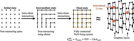The general idea is illustrated in Figure 6 for the example of a $5\times 5$-FBC-system.

Initially, the number of $N_{\mathrm{spins}}=N^2$ non-interacting spins corresponding to the desired $N\times N$-system is placed on the lattice (=initial state 0). As a first step, a total of $N(N-1)$ interactions are added by summarizing the spins to N non-interacting, i.e., independent Ising chains as shown in Figure 6 (=state 1). In this scheme, the chains are labeled beginning from chain-ID 1, corresponding to the minimal length of 1 (i.e., a single spin) to chain-ID N, corresponding to the longest chain, consisting of $2N-1$ spins. In this notion, the added $N(N-1)$ interactions correspond to intra-chain bonds since they connect neighboring spins within a chain. For the remainder of the work, the expressions “interactions” and “bonds” are used synonymously. In order to obtain a fully connected 2D-Ising system, another equal amount of $N(N-1)$ interactions have to be added to the graph, corresponding to inter-chain bonds since they establish interactions between adjacent chains, i.e., to couple neighboring spins assigned to different chains. This could be performed in a series of steps by successively adding more layers of inter-chain bonds. A specific example is shown in Figure 6 where chains are connected via a set of edge bonds such that the edge spin of chain i is connected via 2 bonds to 2 spins of chain $i+1$, resulting in a weakly coupled graph (=state 2). We emphasize that this procedure to go from state 1 (non-interacting Ising chains) to the final state of a fully coupled $N\times N$-system is by no means unique, i.e., there are several ways of adding the remaining $N(N-1)$ inter-chain bonds and as it turns out, this part represents the actual challenge. From a statistical-mechanical point of view, the described approach (denoted by superscript “app.”) corresponds to a free energy construction of the kind:

$$\begin{array}{ccc}\hfill A_{N\times N}^{\mathrm{app}.}& =& A_{\mathrm{chains}}+\sum _{k=1}^m{n}_k\Delta A_{\mathrm{bond}}^{\left(k\right)}\hfill \\ & =& A_{\mathrm{chains}}+n_1\Delta A_{\mathrm{bond}}^{(k=1)}+n_2\Delta A_{\mathrm{bond}}^{(k=2)}+\dots +n_m\Delta A_{\mathrm{bond}}^{(k=m)}.\hfill \end{array}$$

(11)

In such an additive construction scheme, the final free energy estimate $A_{N\times N}^{\mathrm{app}.}$ for the interacting $N\times N$-system results from addition of different free energy contributions $\Delta A_{\mathrm{bond}}^{\left(k\right)}$, associated with the inclusion of specific inter-chain bonds of type k to the reference system of non-interacting Ising chains $A_{\mathrm{chains}}$. If $\Delta A_{\mathrm{bond}}^{\left(k\right)}$ represents the free energy contribution for the addition of a single bond of type k, the corresponding coefficients $n_k$ have to add up to the total number of remaining inter-chain bonds: ${\sum }_{k=1}^m{n}_k=N(N-1)$. Explicit expressions for $A_{\mathrm{chains}}$ and $\Delta A_{\mathrm{bond}}^{\left(k\right)}$ will be derived in the following. Ideally, the constructed $A_{N\times N}^{\mathrm{app}.}$ would correspond to the exact $A_{N\times N}$ for the $N\times N$-FBC-system as calculated from the corresponding exact 2D-partition function based on Equation (2). Equation (11) can be equivalently formulated in terms of partition functions:

$$Z_{N\times N}^{\mathrm{app}.}=Z_{\mathrm{chains}}·{\left(z_{\mathrm{bond}}^{(k=1)}\right)}^{n_1}·{\left(z_{\mathrm{bond}}^{(k=2)}\right)}^{n_2}·\dots ·{\left(z_{\mathrm{bond}}^{(k=m)}\right)}^{n_m}$$

(12)

with the relations $A_{N\times N}^{\mathrm{app}.}=-k_{\mathrm{B}}Tln{Z}_{N\times N}^{\mathrm{app}.}$, $A_{\mathrm{chains}}=-k_{\mathrm{B}}Tln{Z}_{\mathrm{chains}}$ and $\Delta A_{\mathrm{bond}}^{\left(k\right)}=-k_{\mathrm{B}}Tln{z}_{\mathrm{bond}}^{\left(k\right)}$. From the latter relation it follows that $z_{\mathrm{bond}}^{\left(k\right)}$ actually does not represent an absolute partition function but rather a partition function ratio corresponding to the inclusion of a single bond of type k into the graph which is emphasized by the use of a lowercase letter z.

3.1. Free Energy of Independent Ising Chains

The first step corresponding to state 1 in Figure 6 is to summarize the $N^2$ non-interacting spins on the lattice to N independent Ising chains which implies the inclusion of $N(N-1)$ intra-chain bonds to the graph. The first and smallest chain has a length of 1, i.e., an isolated spin while the last chain N is the longest with a length of $2N-1$ spins. Since the chains are independent, the combined partition function for the whole set of N chains is given exactly by the product of the partition functions of the individual chains, i.e., it factorizes into N partition functions:

$$Z_{\mathrm{chains}}=\prod _{k=0}^{N-1}{Z}_{2k+1}^{1\mathrm{D},\mathrm{FBC}}=\prod _{k=1}^N{Z}_{2k-1}^{1\mathrm{D},\mathrm{FBC}}=Z_1·Z_3^{1\mathrm{D},\mathrm{FBC}}·\dots ·Z_{2N-1}^{1\mathrm{D},\mathrm{FBC}}$$

(13)

with $Z_N^{1\mathrm{D},\mathrm{FBC}}=2^N{\cosh }^{N-1}\left(\beta J\right)$ according to Equation (A11a) where the special case $Z_1\equiv Z_1^{1\mathrm{D},\mathrm{FBC}}=2$ corresponds to the partition function of a single isolated spin. In terms of free energy, the corresponding expression reads as:

$$A_{\mathrm{chains}}=\sum _{k=0}^{N-1}{A}_{2k+1}^{1\mathrm{D},\mathrm{FBC}}=\sum _{k=1}^N{A}_{2k-1}^{1\mathrm{D},\mathrm{FBC}}=A_1+A_3^{1\mathrm{D},\mathrm{FBC}}+\dots +A_{2N-1}^{1\mathrm{D},\mathrm{FBC}}$$

(14)

with $A_N^{1\mathrm{D},\mathrm{FBC}}=-k_{\mathrm{B}}Tln{Z}_N^{1\mathrm{D},\mathrm{FBC}}$ according to Equation (A12a) and $A_1\equiv A_1^{1\mathrm{D},\mathrm{FBC}}=-k_{\mathrm{B}}Tln2$. Using the Gaussian sum formula, Equation (14) can be simplified to give the following expression for the (reduced) free energy:

$$\begin{array}{}\mathrm{(15a)}& \hfill A_{\mathrm{chains}}& =-k_{\mathrm{B}}T\left(N^{2}ln2+N(N-1)ln\left(cosh\left(\beta J\right)\right)\right)\hfill \mathrm{(15b)}& \hfill a_{\mathrm{chains}}^{*}& =-ln2-\left(1-\frac{1}{N}\right)ln\left(cosh\left(\beta J\right)\right)\hfill \end{array}$$

which is identical to the expression for the reduced free energy per spin of a single 1D-Ising chain of length N with FBC (compare Equation (A12c)).

3.2. Inclusion of Inter-Chain Interactions

In this work, we applied a simplified variant of the presented approach discussed above where only one bond type in Equation (11) with a single value for the free energy contribution $\Delta A_{\mathrm{bond}}$ is considered. In this case, one adds all inter-chain bonds simultaneously and thus transitions directly from state 1 to the final state of a fully connected $N\times N$-system without any intermediate steps (compare Figure 6):

$$\begin{array}{cc}\hfill A_{N\times N}^{\mathrm{app}.}& =A_{\mathrm{chains}}+N(N-1)\Delta A_{\mathrm{bond}}\hfill \end{array}$$

(16a)

$$\begin{array}{cc}\hfill a_{N\times N}^{*\mathrm{app}.}& =a_{\mathrm{chains}}^{*}+\left(1-\frac{1}{N}\right)\beta \Delta A_{\mathrm{bond}}\hfill \end{array}$$

(16b)

where $a_{\mathrm{chains}}^{*}$ is given by Equation (15b). For the $5\times 5$-FBC-system in Figure 6 this would correspond to the addition of 20 equal bonds to the graph in state 1, where the free energy contribution of each added bond is identical and given by $\Delta A_{\mathrm{bond}}$. At this point it should be stressed that although only one bond type is considered, $\Delta A_{\mathrm{bond}}(\beta ,N)$ is not a constant, but a function of N and $\beta$. Further, it should be emphasized that the decomposition of the free energy into an intra-chain and an inter-chain part does not involve any approximation so far and is exact (i.e., $a_{N\times N}^{*\mathrm{app}.}=a_{N\times N}^{*}$) as long as one calculates the bond contribution $\Delta A_{\mathrm{bond}}$ consistently:

$$\Delta A_{\mathrm{bond}}/J=T^{*}\frac{N}{N-1}\left(a_{N\times N}^{*\mathrm{app}.}-a_{\mathrm{chains}}^{*}\right)$$

(17)

with $T^{*}=k_{\mathrm{B}}T/J$. For infinite lattice size, the equation changes into:

$$\Delta A_{\mathrm{bond}}^{\infty }/J=T^{*}\left(a_{\infty }^{*}-a_{\mathrm{chains},\infty }^{*}\right)$$

(18)

where $\Delta A_{\mathrm{bond}}^{\infty }$ is now a function of temperature only, $a_{\infty }^{*}$ is given by the Onsager expression Equation (7) and $a_{\mathrm{chains}}^{*},\infty =-ln\left(2cosh\left(\beta J\right)\right)$. From the comparison of the Onsager expression with Equation (16b), it can be seen that the second term of the latter equation which involves $\Delta A_{\mathrm{bond}}$ should be given by the integral of the Onsager expression in case of $N\to \infty$ and is thus responsible for the phase transition.

Based on Equation (16b), an equivalent decomposition can also be obtained for the heat capacity via $c^{*}=-{\beta }^2\left({\partial }^2{a}^{*}/\partial {\beta }^2\right)$:

$$\begin{array}{cc}\hfill c_{N\times N}^{*\mathrm{app}.}& =c_{\mathrm{chains}}^{*}+\left(1-\frac{1}{N}\right)\Delta c_{\mathrm{bond}}^{*}\hfill \end{array}$$

(19a)

$$\begin{array}{cc}\hfill & =\left(1-\frac{1}{N}\right)\frac{{\left(\beta J\right)}^2}{{cosh}^2\left(\beta J\right)}-\left(1-\frac{1}{N}\right){\beta }^2{\left(\frac{{\partial }^2(\beta \Delta A_{\mathrm{bond}})}{\partial {\beta }^2}\right)}_N\hfill \\ \hfill & \mathrm{with}{\left(\frac{{\partial }^2(\beta \Delta A_{\mathrm{bond}})}{\partial {\beta }^2}\right)}_N=2{\left(\frac{\partial \Delta A_{\mathrm{bond}}}{\partial \beta }\right)}_N+\beta {\left(\frac{{\partial }^2\Delta A_{\mathrm{bond}}}{\partial {\beta }^2}\right)}_N\hfill \end{array}$$

(19b)

where $c_{\mathrm{chains}}^{*}$ was derived from Equation (15b). For infinite lattice size this expression becomes:

$$\begin{array}{cc}\hfill c_{\infty }^{*\mathrm{app}.}& =c_{\mathrm{chains},\infty }^{*}+\Delta c_{\mathrm{bond},\infty }^{*}\hfill \end{array}$$

(20a)

$$\begin{array}{cc}\hfill & =\frac{{\left(\beta J\right)}^2}{{cosh}^2\left(\beta J\right)}-{\beta }^2{\left(\frac{{\partial }^2(\beta \Delta A_{\mathrm{bond}}^{\infty })}{\partial {\beta }^2}\right)}_N\hfill \end{array}$$

(20b)

where $c_{\infty }^{*\mathrm{app}.}$ only depends on $\beta$.

From the derived expressions it becomes evident that the initial problem of expressing the free energy of a (finite-size) 2D-Ising model by means of 1D-Ising chains is now reduced to the estimation of $\Delta A_{\mathrm{bond}}(\beta ,N)$ as function of system size N and (inverse) temperature $\beta$. A requirement for the calculation of $c_{N\times N}^{*\mathrm{app}.}$ is that the function $\Delta A_{\mathrm{bond}}(\beta ,N)$ is two times differentiable with respect to $\beta$. The route taken in this work was to compute $\Delta A_{\mathrm{bond}}$ according to Equation (17) from the exact $a^{*}$ for a couple of finite-size $N\times N$-systems and then perform an approximation based on a two-dimensional fit in N- and $\beta$-space. For the calculation of $a^{*}$, we used the optimized code of Karandashev et al. [27] which evaluates the exact partition function Z of a given 2D-Ising model at specified temperature and is publically available [28]. Since the code returns $lnZ\left({\beta }^{*}\right)$, $lnZ({\beta }^{*}+\Delta {\beta }^{*})$ and $lnZ({\beta }^{*}+2\Delta {\beta }^{*})$ with $\Delta {\beta }^{*}={10}^{-5}$, the (reduced) heat capacity was computed from a finite-differences (second-order forward) approach. We validated this code for small system dimensions through comparison with self-written (non-optimized) code which evaluates the exact partition functions of $N_y\times N_x$-systems based on the DOS formalism by systematically generating all possible ${\Omega }_{\mathrm{tot}}=2^{N_{\mathrm{spins}}}=2^{N_x·N_y}$ configurations using the Python itertools-module [29]. Relative deviations in $a^{*}$ between the two implementations for the considered temperature range were found to be in the order of ${10}^{-13}$.

Among different investigated modeling approaches for $\Delta A_{\mathrm{bond}}(\beta ,N)$, the following has been found to be the most suitable: (i) calculation of exact values for $\Delta A_{\mathrm{bond}}$ according to Equation (17) for a couple of $N\times N$-systems (e.g., $2\times 2$ to $20\times 20$) within a defined discretized (inverse) temperature interval; (ii) fitting the results with the inverse power law or generalized hyperbola function Equation (21a) in N-space with the four temperature-dependent model parameters $a,b,c,d$, separately for every discrete $\beta$-value (the reader has to be aware of not to confuse the model parameter a with the reduced free energy $a^{*}$):

$$\begin{array}{cc}\hfill \Delta A_{\mathrm{bond}}^{\mathrm{fit}}({\beta }^{*},N)/J& =\frac{a\left({\beta }^{*}\right)}{{(N-b\left({\beta }^{*}\right))}^{c\left({\beta }^{*}\right)}}+d\left({\beta }^{*}\right)\hfill \end{array}$$

(21a)

$$\begin{array}{cc}\hfill {\left(\frac{\partial \Delta A_{\mathrm{bond}}^{\mathrm{fit}}/J}{\partial {\beta }^{*}}\right)}_N& =\frac{a^{\prime }}{{(N-b)}^c}+\frac{ac{b}^{\prime }}{{(N-b)}^{c+1}}-\frac{aln(N-b)c^{\prime }}{{(N-b)}^c}+d^{\prime }\hfill \end{array}$$

(21b)

$$\begin{array}{cc}\hfill {\left(\frac{{\partial }^2\Delta A_{\mathrm{bond}}^{\mathrm{fit}}/J}{\partial {\beta }^{*2}}\right)}_N& =\left[1\right]·a^{\prime }+\left[2\right]·b^{\prime }+\left[3\right]·c^{\prime }\hfill \\ \hfill & +\frac{a^{\prime \prime }}{{(N-b)}^c}+\frac{ac{b}^{\prime \prime }}{{(N-b)}^{c+1}}-\frac{aln(N-b)c^{\prime \prime }}{{(N-b)}^c}+d^{\prime \prime }\hfill \end{array}$$

(21c)

with ${\beta }^{*}=\beta J$, $a^{\prime }\left({\beta }^{*}\right)=\mathrm{d}a/\mathrm{d}{\beta }^{*}$ and $a^{″}\left({\beta }^{*}\right)={\mathrm{d}}^{2}a/\mathrm{d}{\beta }^{*2}$ (analogously for the other model parameters $b,c,d$) and the following abbreviations:

$$\begin{array}{}\mathrm{(22a)}& \hfill \left[1\right]& =\frac{c{b}^{\prime }}{{(N-b)}^{c+1}}-\frac{c^{\prime }ln(N-b)}{{(N-b)}^c}\hfill \mathrm{(22b)}& \hfill \left[2\right]& =\frac{c{a}^{\prime }}{{(N-b)}^{c+1}}+\frac{ac(c+1)b^{\prime }}{{(N-b)}^{c+2}}-\frac{ac{c}^{\prime }ln(N-b)}{{(N-b)}^{c+1}}+\frac{a{c}^{\prime }}{{(N-b)}^{c+1}}\hfill \mathrm{(22c)}& \hfill \left[3\right]& =-\frac{a^{\prime }ln(N-b)}{{(N-b)}^c}+\frac{a{c}^{\prime }{(ln(N-b))}^2}{{(N-b)}^c}+\frac{a{b}^{\prime }}{{(N-b)}^{c+1}}-\frac{ac{b}^{\prime }ln(N-b)}{{(N-b)}^{c+1}}.\hfill \end{array}$$

As can be seen from Equation (21a), for positive exponent c, the asymptotic value of $\Delta A_{\mathrm{bond}}^{\mathrm{fit}}$ for infinite lattice dimension is given by the temperature-dependent offset parameter d: $\Delta A_{\mathrm{bond}}^{\infty \mathrm{fit}}/J\equiv \Delta A_{\mathrm{bond}}^{\mathrm{fit}}({\beta }^{*},\infty )/J=d\left({\beta }^{*}\right)$; (iii) interpolation of the discretized model parameter values in $\beta$-space using cubic splines. Using Equations (21a)–(21c) and (22a)–(22c), the reduced free energy and heat capacity can then be calculated according to Equation (16b) and Equation (19b), respectively, at any temperature and system size.

The quality of the predicted approximations was assessed through a comparison with the exact results for $a^{*}$ and $c^{*}$ as obtained with the code of Karandashev et al. As mentioned above, alternative and lower-complexity modeling approaches for $\Delta A_{\mathrm{bond}}^{\mathrm{fit}}({\beta }^{*},N)/J$, such as a second-degree polynomial function in inverse lattice dimension $N_{\mathrm{inv}}\equiv 1/N$ with only three ${\beta }^{*}$-dependent model parameters were also tested but found not to be suitable (data not shown). Nonlinear fitting of Equation (21a) was performed using the optimize-package of the open-source Python library SciPy [30]. For piecewise cubic splines interpolation, the SciPy interpolate-package has been used. The routine returns not only the interpolated function value itself for the fitting parameters (e.g., $a\left({\beta }^{*}\right)$) but also the corresponding first ($a^{\prime }\left({\beta }^{*}\right)$) and second derivative ($a^{″}\left({\beta }^{*}\right)$) at this temperature as required for the evaluation of Equations (21b), (21c) and (22a)–(22c). At this point, it should be emphasized again that the approximation of the modeling approach is introduced by specifying a specific functional form for $\Delta A_{\mathrm{bond}}^{\mathrm{fit}}({\beta }^{*},N)/J$ (in our case the generalized hyperbola Equation (21a)) and not through Equations (16a), (16b) which are exact. For the sake of completeness, it should be noted that the analytical expression $\Delta A_{\mathrm{bond}}^{\mathrm{fit}}({\beta }^{*},N)/J$ further enables a direct and straightforward calculation of the chemical potential ${\mu }_{N\times N}^{*\mathrm{app}.}$ for arbitrary quadratic systems as function of lattice size and temperature (see Appendix A.4).

4. Results and Discussion

Figure 7 demonstrates the success of the described modeling procedure for $\Delta A_{\mathrm{bond}}(\beta ,N)$ (see methods section for details) involving fitting with the hyperbola-based approach in Equation (21a) to system sizes $2\times 2$ to $20\times 20$. Therefore, exact reference solutions for $\Delta A_{\mathrm{bond}}$ were calculated for these systems using the code of Karandashev et al. [27] at 200 equidistant temperature points in the interval $\beta J=[0.01,2]$ for each system. The shown results for systems $21\times 21$ to $40\times 40$ were not incorporated into the fitting process and thus represent (interpolated) predictions. However, it has been found that it is also necessary to prescribe the Onsager solution for infinite N by constraining the offset parameter d of the fitting function via: $\Delta A_{\mathrm{bond}}^{\mathrm{fit}}({\beta }^{*},\infty )/J=d\left({\beta }^{*}\right)=T^{*}\left(a_{\infty }^{*}-a_{\mathrm{chains},\infty }^{*}\right)$ where Equation (18) has been applied in the second equality. By doing this, d becomes fixed such that only three free adjustable model parameters ($a,b,c$) remain. Without constraining d, the (reduced) heat capacity profile will become unphysical for increasing N and will not converge towards the correct Onsager solution in thermodynamic limit (see Figure A4 in the Appendix A.5). Furthermore, the exponent c was restricted to positive values. As can be seen from Figure 7, $\Delta A_{\mathrm{bond}}^{\mathrm{fit}}$ shows a pronounced dependence on system size and temperature, both of which seem to be well reproduced by our approach. As expected, the free energy contribution of an added bond diminishes with increasing temperature.

The corresponding adjusted model parameters are shown in Figure 8 as function of inverse temperature. It can be seen that all parameters are bound and well-behaved within the studied temperature-range.

Figure 9 shows the modeling results for the reduced free energy per spin $a^{*}$ and reduced heat capacity per spin $c^{*}$ based on Equation (16b) and Equation (19b), respectively, as functions of inverse temperature for selected $N\times N$-systems. By construction through constraining the model parameter d, both $a^{*}$ and $c^{*}$ become identical to the corresponding Onsager expressions for $N\to \infty$. While the agreement between the tested model approach and corresponding exact results are close to perfect in case of $a^{*}$, a fact which is also confirmed by the very low percentage relative deviation ($<0.1\%$) in Figure 10, deviations for $c^{*}$ are more pronounced. This behavior is due to the fact that $c^{*}$ is proportional to the second derivative of $a^{*}$ and thus is very sensitive to small local changes in the curvature of $a^{*}\left({\beta }^{*}\right)$. For all system sizes, some artifacts are present in $c^{*}$ around the critical temperature which cause the curves to become increasingly rugged near the maximum as N increases and makes an unambiguous determination of the peak maximum and the corresponding peak temperature difficult. These numerical artifacts can be mainly attributed to two origins: (i) a side effect of the imposed constraint to match the Onsager solution for infinite N and (ii) the limited number of temperature points as used for interpolation. The latter can be seen when more temperature points are used which increases the resolution in $\beta$-space at the expense of increased computational effort. Although a higher $\beta$-resolution reduces the artifacts near the critical temperature and makes the curves smoother around the maximum, this creates small local disturbances (see Figure A5 in the Appendix A.5). For large N-values outside the fitting range, the maximum of the approximated $c^{*}$-curve is already determined by the critical temperature ${\beta }_c^{*}={\beta }_{c}J={(k_{\mathrm{B}}{T}_c/J)}^{-1}\approx 0.44$, whereas the peak temperature of the exact curve does not yet match it (see result for the $40\times 40$-system in Figure 9b). However, despite these deviations in the shape of the profiles, the evaluation of the integral conditions in Equations (10a), (10b) yielded a maximal violation in the order of $1\%$ from the nominal value. In this context, the impact of including the exact results from more $N\times N$-systems in the fitting process at the same temperature resolution was also investigated (see Figure A6 in the Appendix A.5). For small system sizes the aforementioned artifacts close to ${\beta }_c^{*}$ become more pronounced when more systems were taken into account for fitting (at same $\beta$-resolution) while for the prediction of larger system sizes the description near the peak becomes better. However, the qualitative behavior is identical for the studied cases where a different number of reference solutions was involved. Figure 10 further shows that the deviations in $a^{*}$ disappear for very high and low temperatures at all system sizes. Although it appears that local extrema emerge at certain intervals which increase with increasing N, in the limiting case for infinite N, all deviations must by construction decrease to zero for all temperatures.

As already mentioned in the introduction, a separate publication will focus on the adaption of the Ising model such that it can be applied to the description of intercalation phenomena such as the intercalation of Li-ions into an electrode host matrix. Here, we will only briefly illustrate a possible roadmap for such a modeling attempt. In the simplest case, one could study a one-dimensional cut through a (finite-sized) crystal lattice composed of N lattice sites where each site can be either occupied by an ion ($s_i=1$) or empty ($s_i=0$). Such a description could be used for example to model the diffusion of Li-ions diffusion into tunnel-like structures of ${\mathrm{LiFePO}}_4$ [31,32]. Therefore, a Hamiltonian based on pairwise ion-ion interactions could be constructed in the following way:

$$\begin{array}{ccc}\hfill H_N^{1\mathrm{D},\mathrm{FBC}}& =& \sum _{i=1}^{N-1}\sum _{j=i+1}^N{ϵ}_{i,j}\hfill \\ & =& \underset{\mathrm{N}-1\mathrm{terms}}{\underbrace{\{{ϵ}_{1,2}+{ϵ}_{2,3}+\dots +{ϵ}_{N-1,N}\}}}+\underset{\mathrm{N}-2\mathrm{terms}}{\underbrace{\{{ϵ}_{1,3}+{ϵ}_{2,4}+\dots +{ϵ}_{N-2,N}\}}}+\dots +\underset{1\mathrm{term}}{\underbrace{\left\{{ϵ}_{1,N}\right\}}}\hfill \end{array}$$

(23)

with the pair energy ${ϵ}_{i,j}=J_{i,j}{s}_i{s}_j$ between lattice sites i and j. Equation (23) involves a total of $N(N-1)/2$ pair interactions in case of FBC, comprising $N-1$ possible nearest neighbor interactions between adjacent lattice sites, $N-2$ possible next-nearest neighbor interactions between lattice sites which have another site in between and so on. Due to the long-range nature of electrostatic interactions it might be necessary to include interactions which go beyond nearest neighbors which is a clear difference compared to the classic Ising model (compare Equation (A1a)) and the simplifying assumption of a uniform coupling constant $J_{i,j}$ might not be applicable. A possible modeling approach of the distance-dependence of $J_{i,j}$ for interaction sites which are $n\ge 1$ sites apart could be derived in analogy to Coulomb’s law according to $J_{i,i+n}=J/n$. Here, the coupling constant $J\equiv J_{i,i+1}$ between ions sitting directly next to each other (i.e., $s_i=s_{i+1}=1$) could be treated as adjustable model parameter. Another degree of freedom could be introduced by the multiplication of J with a distance-dependent screening parameter ${\alpha }_{i,j}$ to better incorporate the effect of the electrode matrix on the alteration of the ion-ion interactions. For computational reasons it might be necessary to define a certain cut-off distance beyond which the interactions are assumed to be zero which can be included into ${\alpha }_{i,j}$ in combination with a special switching function. Of course, both $J_{i,j}$ and ${\alpha }_{i,j}$ could further be treated as temperature-dependent. Due to the inherent periodicity of the crystal, inclusion of PBC might yield a more realistic description for finite-size systems. For a 1D-crystal with N lattice sites, the corresponding canonical partition function $Z_N^{1\mathrm{D}}$ involves a total of ${\Omega }_{\mathrm{tot}}=2^N$ possible configurations, including states with $0,1,\cdots ,N$ ions and can (in principle) be calculated for every lattice size according to Equation (2). In 1D, the transfer matrix method offers a route to obtain a closed analytic solution for $Z_N$ [33]. However, in order to apply this kind of model for intercalation of Li-ions into other host materials where two- or three-dimensional diffusion takes place such as graphitic carbon [34] or ${\mathrm{LiMn}}_2{\mathrm{O}}_4$ spinel [35], respectively, efficient approximative approaches for the evaluation of the higher-dimensional Ising model are required which was the main motivation of the present work. For these situations, a similar approach as presented in this work will be followed, comprising calculation of exact partition functions (or free energies $A_{N\times N}$) for a couple of finite-size $N\times N$-systems, followed by approximation of $A_{N\times N}$ with a suitable analytic expression and extrapolation to other lattice dimensions of interest. In contrast to the classic Ising model, it is known that such a proposed model based on the Hamiltonian above features a phase transition even in 1D due to the presence of long-range interactions [36,37]. The advantages of such a simple but at the same time physically based model and its implications for battery modeling are versatile: it could be used not only to predict the most probable electrode composition at a particular temperature but also transition temperatures between different phases from the heat capacity profile. Through the combination with experimentally or computationally determined ionic conductivities or diffusion coefficients, a link to transport properties of ionic species within crystal lattices can be achieved. Microscopic origins of hysteresis effects during dis-/charging which are highly relevant for battery energy efficiency and are thought to be related to lattice reorganization, could be possibly incorporated into such a model through further factorization of the coupling constant.

5. Conclusions

The central question addressed in this work was whether it is possible to develop a free energy expression on the basis of 1D-Ising chains that can reproduce the results of a finite-size 2D-Ising model with FBC at least qualitatively. Therefore, we considered an arbitrary $N\times N$-system as a combination of an intra-chain part which is given by a set of non-interacting Ising chains and an inter-chain part through which interactions among neighboring chains are established. In this context we considered the free energy contribution of a single inter-chain bond $\Delta A_{\mathrm{bond}}(\beta ,N)$ that is added to the system and shows a distinct dependence on (inverse) temperature and lattice size. It could be shown that with the chosen modeling approach based on 1D-Ising chains in combination with an analytic expression for $\Delta A_{\mathrm{bond}}$ for which the involved model parameters were adjusted to exact results from a couple of finite-size 2D-systems, a satisfying reproduction of the exact data in terms of $\Delta A_{\mathrm{bond}}(\beta ,N)$ can be achieved. However, extrapolation to lattices, which are significantly larger than those included for the fit, is only possible when the limiting solution for infinite N is explicitly incorporated into the fitting step. This is especially true for the reduced heat capacity per spin (to a much lesser extent for the reduced free energy per spin), which is as a second-derivative property extremely sensitive to subtle local changes in curvature of $a^{*}$. This shows the limitation of the current approach which could be attributed to the particularly chosen fitting approach. However, it must be emphasized that the primary goal of the current work was not to find an optimal working approach that reproduces the exact results as closely as possible, but to show a principal (qualitative) route for how such a model could be built. Based on the obtained results, we will extend the modeling approach by trying to split the process of adding inter-chain bonds to the system of non-interacting Ising chains into different intermediate steps as it is illustrated in Figure 6 which will then also be tested for the 3D-Ising model.

References

1. Lenz, W. Beitrag zum Verständnis der magnetischen Erscheinungen in festen Körpern. Phys. Z. 1920, 21, 613–615. [Google Scholar]
2. Ising, E. Beitrag zur Theorie des Ferromagnetismus. Z. Phys. 1925, 31, 253–258. [Google Scholar] [CrossRef]
3. Lipowski, A. Ising model: Recent developments and exotic applications. Entropy 2022, 24, 1834. [Google Scholar] [CrossRef]
4. Pan, A.C.; Chandler, D. Dynamics of nucleation in the Ising model. J. Phys. Chem. B 2004, 108, 19681–19686. [Google Scholar] [CrossRef]
5. De Oliveira, M.; Griffiths, R.B. Lattice-gas model of multiple layer adsorption. Surf. Sci. 1978, 71, 687–694. [Google Scholar] [CrossRef]
6. Stauffer, D. Social applications of two-dimensional Ising models. Am. J. Phys. 2008, 76, 470–473. [Google Scholar] [CrossRef]
7. Tarascon, J.M.; Armand, M. Issues and challenges facing rechargeable lithium batteries. Nature 2001, 414, 359–367. [Google Scholar] [CrossRef]
8. Viswanathan, G.M.; Portillo, M.A.G.; Raposo, E.P.; da Luz, M.G. What does it take to solve the 3D Ising model? Minimal necessary conditions for a valid solution. Entropy 2022, 24, 1665. [Google Scholar] [CrossRef] [PubMed]
9. Fisher, M.E.; Selke, W. Infinitely many commensurate phases in a simple Ising model. Phys. Rev. Lett. 1980, 44, 1502. [Google Scholar] [CrossRef]
10. Potts, R.B. Some generalized order-disorder transformations. In Mathematical Proceedings of the Cambridge Philosophical Society; Cambridge University Press: Cambridge, UK, 1952; Volume 48, pp. 106–109. [Google Scholar]
11. Scheck, F. Theoretische Physik 5: Statistische Theorie der Wärme; Springer: Berlin/Heidelberg, Germany, 2008. [Google Scholar]
12. Newell, G.F.; Montroll, E.W. On the theory of the Ising model of ferromagnetism. Rev. Mod. Phys. 1953, 25, 353. [Google Scholar] [CrossRef]
13. Brush, S.G. History of the Lenz-Ising model. Rev. Mod. Phys. 1967, 39, 883. [Google Scholar] [CrossRef]
14. Landau, D.P.; Wang, F. A new approach to Monte Carlo simulations in statistical physics. Braz. J. Phys. 2004, 34, 354–362. [Google Scholar] [CrossRef]
15. Janke, W. Monte Carlo simulations in statistical physics—From basic principles to advanced applications. In Order, Disorder and Criticality: Advanced Problems of Phase Transition Theory Volume 3; World Scientific: Singapore, 2013; pp. 93–166. [Google Scholar]
16. Onsager, L. Crystal statistics. I. A two-dimensional model with an order-disorder transition. Phys. Rev. 1944, 65, 117–149. [Google Scholar] [CrossRef]
17. Kaufman, B. Crystal statistics. II. Partition function evaluated by spinor analysis. Phys. Rev. 1949, 76, 1232. [Google Scholar] [CrossRef]
18. Ferdinand, A.E.; Fisher, M.E. Bounded and inhomogeneous Ising models. I. Specific-heat anomaly of a finite lattice. Phys. Rev. 1969, 185, 832. [Google Scholar] [CrossRef]
19. Beale, P.D. Exact distribution of energies in the two-dimensional Ising model. Phys. Rev. Lett. 1996, 76, 78. [Google Scholar] [CrossRef]
20. Binder, K. Statistical mechanics of finite three-dimensional Ising models. Physica 1972, 62, 508–526. [Google Scholar] [CrossRef]
21. Kim, S.Y. Ising model on L× L square lattice with free boundary conditions up to L= 19. J. Phys. Conf. Ser. 2013, 410, 012050. [Google Scholar] [CrossRef]
22. Carra, J.H.; Murphy, E.C.; Privalov, P.L. Thermodynamic effects of mutations on the denaturation of T4 lysozyme. Biophys. J. 1996, 71, 1994–2001. [Google Scholar] [CrossRef]
23. Karandashev, I.M.; Kryzhanovsky, B.V.; Malsagov, M.Y. Analytical expressions for a finite-size 2D Ising model. Opt. Mem. Neural Netw. 2017, 26, 165–171. [Google Scholar] [CrossRef]
24. Kramers, H.A. Statistics of the two-dimensional ferromagnet. Part I. Phys. Rev. 1941, 60, 252–262. [Google Scholar] [CrossRef]
25. Landau, D.; Binder, K. A Guide to Monte Carlo Simulations in Statistical Physics; Cambridge University Press: Cambridge, UK, 2009. [Google Scholar]
26. Rehner, P.; Bauer, G. Application of generalized (hyper-) dual numbers in equation of state modeling. Front. Chem. Eng. 2021, 3, 758090. [Google Scholar] [CrossRef]
27. Karandashev, Y.M.; Malsagov, M.Y. Polynomial algorithm for exact calculation of partition function for binary spin model on planar graphs. Opt. Mem. Neural Netw. 2017, 26, 87–95. [Google Scholar] [CrossRef]
28. Implementation 2D-Partition-Function Code. Available online: https://github.com/Thrawn1985/2D-Partition-Function (accessed on 21 April 2023).
29. Van Rossum, G. The Python Library Reference, Release 3.8.2; Python Version 3.9.16; Python Software Foundation: Wilmington, DE, USA, 2020. [Google Scholar]
30. Virtanen, P.; Gommers, R.; Oliphant, T.E.; Haberland, M.; Reddy, T.; Cournapeau, D.; Burovski, E.; Peterson, P.; Weckesser, W.; Bright, J.; et al. SciPy 1.0: Fundamental algorithms for scientific computing in Python. Nat. Methods 2020, 17, 261–272. [Google Scholar] [CrossRef] [PubMed]
31. Ceder, G. Opportunities and challenges for first-principles materials design and applications to Li battery materials. MRS Bull. 2010, 35, 693–701. [Google Scholar] [CrossRef]
32. Chen, G.; Song, X.; Richardson, T.J. Electron microscopy study of the LiFePO4 to FePO4 phase transition. Electrochem.-Solid-State Lett. 2006, 9, A295. [Google Scholar] [CrossRef]
33. Martínez-Herrera, J.; Rodríguez-López, O.A.; Solís, M. Critical temperature of one-dimensional Ising model with long-range interaction revisited. Phys. A Stat. Mech. Appl. 2022, 596, 127136. [Google Scholar] [CrossRef]
34. Persson, K.; Sethuraman, V.A.; Hardwick, L.J.; Hinuma, Y.; Meng, Y.S.; Van Der Ven, A.; Srinivasan, V.; Kostecki, R.; Ceder, G. Lithium diffusion in graphitic carbon. J. Phys. Chem. Lett. 2010, 1, 1176–1180. [Google Scholar] [CrossRef]
35. Xu, B.; Meng, S. Factors affecting Li mobility in spinel LiMn2O4—A first-principles study by GGA and GGA+ U methods. J. Power Sources 2010, 195, 4971–4976. [Google Scholar] [CrossRef]
36. Dyson, F.J. Existence of a phase-transition in a one-dimensional Ising ferromagnet. Commun. Math. Phys. 1969, 12, 91–107. [Google Scholar] [CrossRef]
37. Fröhlich, J.; Spencer, T. The phase transition in the one-dimensional Ising model with 1/r2 interaction energy. Commun. Math. Phys. 1982, 84, 87–101. [Google Scholar] [CrossRef]
38. Göpel, W.; Wiemhöfer, H.D. Statistische Thermodynamik; Springer: Berlin/Heidelberg, Germany, 2000. [Google Scholar]
39. Shannon, C.E. A mathematical theory of communication. Bell Syst. Tech. J. 1948, 27, 379–423. [Google Scholar] [CrossRef]
40. Ben-Naim, A. Information, entropy, life, and the universe. Entropy 2022, 24, 1636. [Google Scholar] [CrossRef] [PubMed]
41. Mueller, M.; Johnston, D.A.; Janke, W. Exact solutions to plaquette Ising models with free and periodic boundaries. Nucl. Phys. B 2017, 914, 388–404. [Google Scholar] [CrossRef]
Figure 1. Calculated densities of states (DOS) for a couple of quadratic ( N × N ) 2D-Ising systems: 2 × 2 (blue), 3 × 3 (green), 4 × 4 (orange), 5 × 5 (red). (a) Free boundary conditions (FBC), (b) periodic boundary conditions (PBC).
Batteries 09 00489 g001
Figure 2. Thermodynamics of 2 × 2 -Ising model with FBC: (a) fractions (=probabilities) p 0 (black), p 1 (blue) and p 2 (red) of finding the system in states with system energy 4 J , 0, and 4 J , respectively, as function of temperature according to Equations (6b)–(6d). High-temperature asymptotic values for T derived from Equations (6b)–(6d) are given by: p 0 ( ) = p 2 ( ) = 0.125 ,   p 1 ( ) = 0.75 . (b) Temperature-dependence of free energy A (black) and decomposition into internal energy U (blue) and entropic part T S (red) according to the Gibbs-Helmholtz equation: A = U T S . All quantities were calculated from the corresponding partition function Equation (4) using Equations (A7a), (A7b) and (A3c). The black dashed line which is shown as guide to the eye corresponds to the high-temperature asymptotic given by k B T ln Ω tot with Ω tot = 2 4 = 16 .
Batteries 09 00489 g002
Figure 3. Thermodynamics of 5 × 5 -Ising model with FBC: (a) fractions (=probabilities) p i of finding the system in one of the 39 distinct energy states (cf. Figure 1a) as function of temperature according to Equation (6a). The 39 curves are colored according to ascending energy levels from E 0 = 40 J (dark blue) to E 38 = 40 J (dark red). The black dashed lines corresponds to state 20 at the maximum of the DOS distribution in Figure 1a with corresponding energy level E 19 = 0 , showing the highest high-temperature asymptotic value ( p 19 ( ) 0.130 ) among all states. (b) Temperature-dependence of free energy A (black) and decomposition into internal energy U (blue) and entropic part T S (red) according to the Gibbs-Helmholtz equation: A = U T S . All quantities were calculated from the corresponding partition function using Equations (A7a), (A7b) and (A3c). The black dashed line which is shown as guide to the eye corresponds to the high-temperature asymptotic given by k B T ln Ω tot with Ω tot = 2 25 3.36 × 10 7 .
Batteries 09 00489 g003
Figure 4. Reduced free energy per spin a * = β A / N spins as function of inverse temperature β J = J / k B T for a couple of quadratic ( N × N ) 2D-Ising systems: 2 × 2 (blue), 3 × 3 (green), 4 × 4 (orange), 5 × 5 (red). (a) Free boundary conditions (FBC), (b) periodic boundary conditions (PBC). For completeness, the Onsager solution for the case of an infinitely sized system according to Equation (7) is also shown (black curve). Dashed lines in (a) correspond to the low-temperature (LT) approximation as applicable for FBC given by a N * LT ( β * ) = 2 β * 1 1 / N with β * = β J [23].
Batteries 09 00489 g004
Figure 5. Reduced heat capacity per spin c * = C / k B N spins as function of temperature for a couple of quadratic ( N × N ) 2D-Ising systems: 2 × 2 (blue), 3 × 3 (green), 4 × 4 (orange), 5 × 5 (red). (a) Free boundary conditions (FBC), (b) periodic boundary conditions (PBC). The corresponding heat capacity for the thermodynamic limit was derived from the Onsager expression for a * in Equation (7) (black curve). The black dashed line corresponds to the critical temperature in the thermodynamic limit ( k B T c / J 2.269 ) as given by Equation (8). The left graph also shows the limiting heat capacity for the 1D-Ising model (fine purple dashed-dotted line).
Batteries 09 00489 g005
Figure 6. Schematic representation of the approach: starting from a system of non-interacting spins for the 2D-topology of interest (=state 0), the spins are first summarized to a set of non-interacting 1D-systems, i.e., Ising chains (=state 1). In the following steps, successive layers of inter-chain interactions (=bonds) between neighboring chains are added sequentially, resulting in a fully connected graph at the final state (here a 5 × 5 -FBC-system).
Batteries 09 00489 g006
Figure 7. Free energy contribution of a single inter-chain bond Δ A bond / J as function of lattice size (left) and temperature (right): (a) circles (closed and open) represent exact solutions for Δ A bond / J calculated according to Equation (17). Dashed lines correspond to fitting results according to Equation (21a) at constant temperature within β J = [ 0.01 , 2 ] using 200 equidistant points. Closed (open) circles represent points that were (not) incorporated into the fitting process. The coloring scheme of the lines refers to ascending order in temperature, with blue curves at the bottom corresponding to low temperature (high β ) and red curves at the top to high temperature (low β ). (b) Δ A bond / J as function of reduced temperature k B T / J for selected N × N -systems: 2 × 2 (blue), 5 × 5 (cyan), 10 × 10 (green), 20 × 20 (orange), 40 × 40 (red). The limiting Onsager solution is shown in magenta. Colored curves correspond to exact results according to Equation (17) whereas superimposed black dashed lines refer to modeling results from (a). The shown 40 × 40 -system (red) was not taken explicitly into account into the fitting process but is a prediction.
Batteries 09 00489 g007
Figure 8. Model parameters a (blue), b (green), c (orange) and d (red) of the generalized hyperbola function for Δ A bond fit / J (see Equation (21a)), corresponding to Figure 7a as function of inverse temperature. For the fitting procedure, the c-parameter was constrained to positive values and the parameter d was not taken as free parameter but constrained to the exact limiting value of Δ A bond / J for N according to Equation (18). The black dashed-dotted line is shown as guide to the eye and corresponds to the inverse critical temperature in the thermodynamic limit ( β c J = ( k B T c / J ) 1 0.44 ) as given by Equation (8).
Batteries 09 00489 g008
Figure 9. Reduced free energy (a) and reduced heat capacity per spin (b) as a function of inverse temperature for selected N × N -systems: 2 × 2 (blue), 5 × 5 (cyan), 10 × 10 (green), 20 × 20 (orange), 40 × 40 (red). The left graph also includes the limiting Onsager solution (magenta). For the fitting procedure, 200 equidistant points within the interval β J = [ 0.01 , 2 ] were applied for system sizes 2 N 20 . Systems with dimensions 21 < N < represent predictions. Colored curves correspond to exact results while black (dashed) lines represent modeling results based on Equations (16b) and (19b), respectively. The black dashed-dotted line in the right graph is shown as guide to the eye and corresponds to the inverse critical temperature in the thermodynamic limit ( β c J = ( k B T c / J ) 1 0.44 ) as given by Equation (8).
Batteries 09 00489 g009
Figure 10. Relative deviation (in percent) between exact and approximated reduced free energy per spin ( a N × N * app . a N × N * ) / | a N × N * | × 100 % as function of inverse temperature for selected N × N -systems (a) and as function of lattice size for specified inverse temperatures (b). a N × N * app . denotes the modeled reduced free energy per spin according Equation (16b) while a N × N * corresponds to the exact reference solution, evaluated via the code of Karandashev et al. [27]. For the fitting procedure, 200 equidistant points within the interval β J = [ 0.01 , 2 ] were applied for system sizes 2 N 20 . Systems with dimensions 21 < N < represent predictions. Shown system sizes in (a): 2 × 2 (blue), 5 × 5 (cyan), 10 × 10 (green), 20 × 20 (orange), 30 × 30 (dark red), 40 × 40 (red). The black dashed-dotted line corresponds to the inverse critical temperature in the thermodynamic limit ( β c J = ( k B T c / J ) 1 0.44 ) as given by Equation (8). Shown isothermes in (b): β J = 0.01 (blue), β J = 0.44 (cyan), β J = 0.50 (green), β J = 0.70 (orange), β J = 1.00 (red), β J = 2.00 (magenta).
Batteries 09 00489 g010
Disclaimer/Publisher’s Note: The statements, opinions and data contained in all publications are solely those of the individual author(s) and contributor(s) and not of MDPI and/or the editor(s). MDPI and/or the editor(s) disclaim responsibility for any injury to people or property resulting from any ideas, methods, instructions or products referred to in the content.