Article

Cell Replacement Strategies for Lithium Ion Battery Packs

by
Nenad G. Nenadic
*,†,
Thomas A. Trabold
and
Michael G. Thurston
Rochester Institute of Technology, Rochester, NY 14623, USA
*
Author to whom correspondence should be addressed.
These authors contributed equally to this work.
Batteries 2020, 6(3), 39; https://doi.org/10.3390/batteries6030039
Submission received: 13 May 2020 / Revised: 29 June 2020 / Accepted: 17 July 2020 / Published: 23 July 2020
(This article belongs to the Special Issue Lithium-Ion Batteries: Latest Advances and Prospects)

Abstract

:
The economic value of high-capacity battery systems, being used in a wide variety of automotive and energy storage applications, is strongly affected by the duration of their service lifetime. Because many battery systems now feature a very large number of individual cells, it is necessary to understand how cell-to-cell interactions can affect durability, and how to best replace poorly performing cells to extend the lifetime of the entire battery pack. This paper first examines the baseline results of aging individual cells, then aging of cells in a representative 3S3P battery pack, and compares them to the results of repaired packs. The baseline results indicate nearly the same rate of capacity fade for single cells and those aged in a pack; however, the capacity variation due to a few degrees changes in room temperature (≃±3 C) is significant (≃±1.5% of capacity of new cell) compared to the percent change of capacity over the battery life cycle in primary applications (≃20–30%). The cell replacement strategies investigation considers two scenarios: early life failure, where one cell in a pack fails prematurely, and building a pack from used cells for less demanding applications. Early life failure replacement found that, despite mismatches in impedance and capacity, a new cell can perform adequately within a pack of moderately aged cells. The second scenario for reuse of lithium ion battery packs examines the problem of assembling a pack for less-demanding applications from a set of aged cells, which exhibit more variation in capacity and impedance than their new counterparts. The cells used in the aging comparison part of the study were deeply discharged, recovered, assembled in a new pack, and cycled. We discuss the criteria for selecting the aged cells for building a secondary pack and compare the performance and coulombic efficiency of the secondary pack to the pack built from new cells and the repaired pack. The pack that employed aged cells performed well, but its efficiency was reduced.

1. Introduction

Large lithium-ion battery packs are emerging in both vehicular and stationary energy storage applications, with rapidly increasing market penetration expected in the coming decades. The extent of battery system commercialization in both vehicle and renewable energy applications will depend upon the environmental and economic benefits that can be realized relative to incumbent technologies and other advanced mobility and energy technologies, such as fuel cells [1]. The effective cost of battery systems can be reduced by amortizing the cost over longer usage cycles. Two ways to extend the usage cycle of battery systems are (1) to extend the life of cells and packs in the original application, and (2) to reuse cells for other applications. For example, several studies have indicated that the cost of plug-in hybrid vehicle battery packs may be offset by repurposing vehicle batteries in grid support systems [2], and some automotive original equipment manufacturers (OEMs) are actively pursuing this option with energy technology companies [3,4]. For vehicle applications, Marano et al. [5] built a general, high-level model and, based on conservative assumptions, estimated that vehicles equipped with lithium ion batteries can last up to 10 years and provide the equivalent of 150,000 miles of travel. For battery packs that have failures or significant capacity loss prior to reaching the expected life-cycle, some means of recapitalization of the cell value is important to the overall cost to benefit ratio. Although many studies have addressed fundamental degradation modes of common battery electrode materials, these studies are often conducted at the “button cell” or single-cell 18650 scale where effects of assembly, packaging, and integration are not fully comprehended. The importance of acquiring a detailed understanding of cell aging, individually and in packs, has been recognized previously, and much recent research has focused on techniques for battery health monitoring and prognostics of battery packs in electric vehicles (e.g., review articles by [6,7,8]). Designing and implementing strategies for first identifying and then isolating failures of individual cells within a pack is challenging, although some potential methods have been proposed [9,10,11,12,13]. Recently, Li et al. [14] proposed three categories of approaches for multicell state estimation:
  • treating the battery pack as a single cell of high voltage and capacity;
  • applying single-cell state-of-charge (SOC) estimation methods to every cell in a pack, but this approach is computationally intensive and cumbersome for practical application;
  • quantifying individual cell SOC by analyzing variations in open circuit voltage and internal resistance.
The difficulty in assessing and comparing many of these advanced battery system-level monitoring approaches is that direct, in-situ data from electric vehicles or storage systems are not readily available in the open literature. Therefore, many researchers have relied on experimental and modeling studies that start with simpler multi-cell systems and then attempt to extrapolate these findings to more complex, commercial-scale systems. Dubarry et al. have reported on cell aging and the degradation mechanisms of a composite positive electrode [15,16]. Understanding the origins of cell variations can be used for building more robust packs [17]. Moreover, it is well known that multi-cell (pack) aging behavior can be quite different from that associated with single cells, due to the need for cell balancing and thermal management, among other effects [18,19]. Thus, it is important to first fully characterize aging behavior at the individual cell level as a function of the pertinent operating parameters and for different electrode materials [20]. The cell characterization can be used for accelerated estimation of remaining capacity and state of charge [21].
In the current research program, after quantifying the aging of individual LiCo 18650 cells at a statistically significant level, the evaluation process was systematically extended to small packs which represent small-scale versions of larger commercial battery systems. Pack-level testing was intended to gain insight into a variety of practical issues associated with commercial battery systems. The selected pack was a 3 × 3 cell arrangement (three cells are connected in series to form a string and then three strings are connected in parallel, i.e., 3S3P configuration), with its associated charging and discharging processes, and enabled comparison of aging of cells in the pack versus individual cell aging. The replacement strategies considered two scenarios.
The first scenario, the replacement of an early life failure, addresses an important open question for maintenance of battery packs. The traditional approach in pack maintenance is to replace all cells at once to control the mismatches. This approach is clearly untenable for very large battery packs. Even for packs built in a hierarchical fashion, where cells are first assembled into sub-modules, which, in turn, form larger modules, this replacement philosophy does not work because replacement of a single cell in a module would require replacement of all the cells in the module, and, by extension of this approach, all the sub-modules, etc. Replacement of all cells as a result of an early-life failure in a large pack is clearly not economically viable; therefore, an alternative strategy needs to be established. One strategy for minimizing imbalance and premature aging in this scenario is to maintain an inventory of cells aged to different levels of capacity fade and to select the appropriately aged cell, or cells, to effect the repair. The experimental results reported here have been obtained on a small pack, which is a module that could be used in larger packs. Since larger packs are built hierarchically, where modules are often treated as larger cells, the conclusions of this study should provide important insight into the behavior of larger packs as well.
The second scenario addresses the problem of secondary uses for the cells in a less demanding application after the end of useful life in a higher-performance application. These cells, while no longer suitable for the original applications, may be deemed adequate for less demanding applications. For example, studies have indicated that the cost of plug-in hybrid vehicle battery packs may be reduced by repurposing vehicle batteries in grid support systems because modules would be sold to the secondary user and the primary user would not have to assume the processing cost associated with safe disposal [2,22,23]. For example, Schneider et al. [24], who developed methods for assessment and reuse of nickel metal hydride (NMH) cells, found that, on average, about 37% of discarded cells have sufficient remaining capacity for reuse. Lih et al. [25] identified technological challenges and analyzed secondary uses of lithium ion batteries from an economic point of view. The potential of lithium ion batteries, after they serve their useful life, for grid applications has been considered by Kamath of the Electric Power Research Institute (EPRI) [26], who hypothesized that cost per production volume may be lower than lead-acid batteries. Neubauer et al. have performed a techno-economic analysis of vehicle batteries for secondary uses [27,28,29]. They concluded that an uninterruptible power supply (UPS) system based on used lithium ion batteries has the potential to be more cost effective than lead-acid batteries, with superior longevity, specific energy, and energy density. The considerable potential for secondary applications has been widely recognized. The present study examines empirically practical problems of maintenance and rebuilding of packs using a small 3 × 3 pack as the platform.

2. Methodology

The objective of the empirical study was twofold: to compare aging of lithium ion cells individually and in small packs and to test investigate cell rebuilding packs in the context of two case studies. This objective was executed by three sets of tests: the first set compared aging of single 1860 LiCo cells to their aging in small packs, the second set examined performance of a used pack after one of the cell was replaced by a new cell and the third set examined scenarios of rebuilding packs from two packs that were considered “failed”. The details of individual set of tests are described in subsequent sub-sections. The main metrics were capacity fade, impedance changes, and coulombic efficiency.
The study employed two test stands: one for single-cell testing and the other for battery pack evaluations. The single-cell apparatus was a Maccor 4600 battery test system, used for initial cell characterization, pre-aging of individual cells, and periodic monitoring of the cells subjected to pack-level cycling. Additional details on the test procedure are provided in the Supplementary Materials.
The test stand for pack testing is shown in Figure 1a. The packs consisted of nine cells in 3S3P configuration: three strings of three serially connected cells were connected in parallel, as shown in Figure 1b. The pack employed passive cell balancing, based on the commercial, off-the-shelf balancing circuit. A diagram of the test stand is depicted in Figure 1c. More details on cell balancing are provided in the Supplementary Materials.

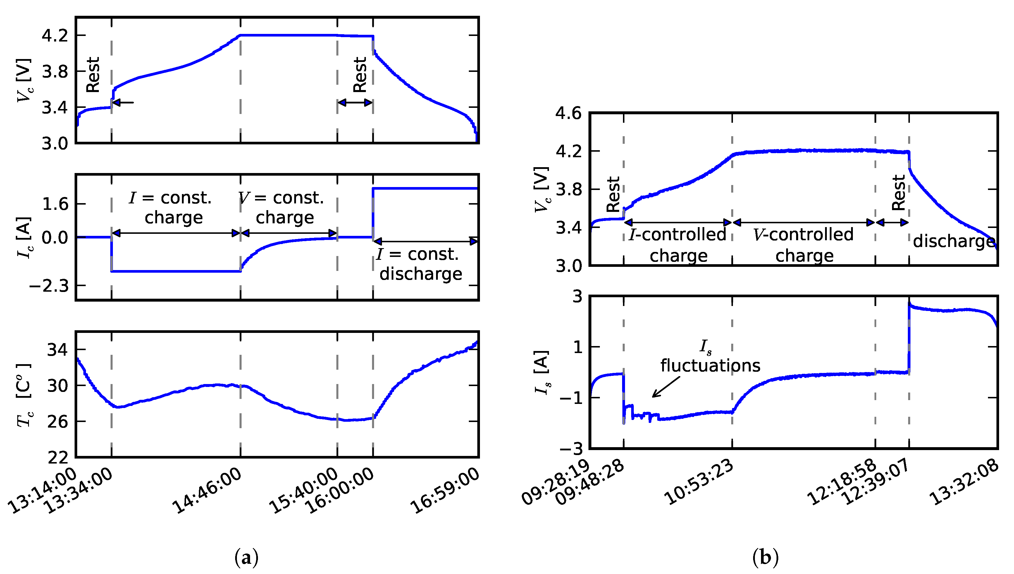
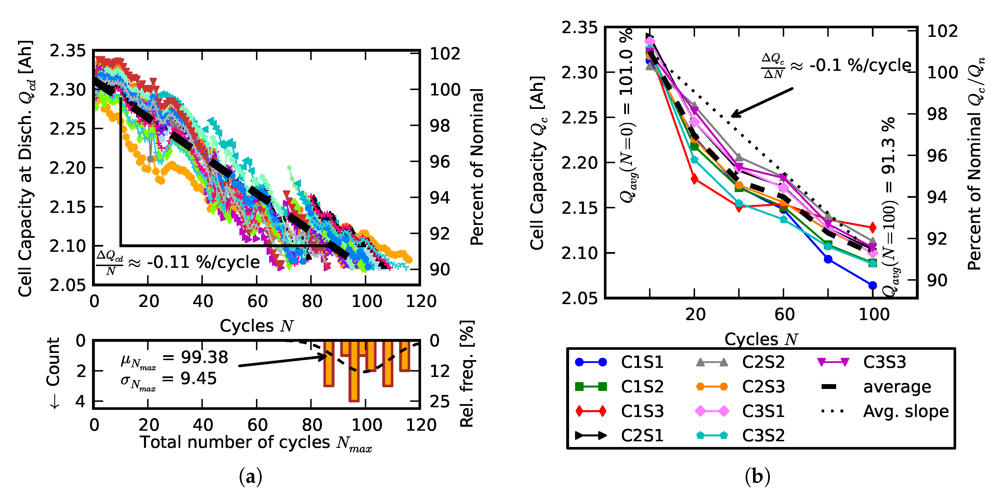
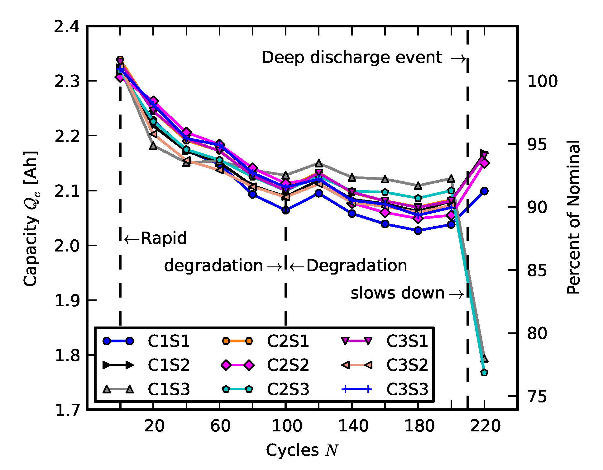
2.1. Individual and Pack Aging of 18650 LiCo Cells

For this study, cell aging was limited to full charge-discharge cycles of battery cells. A typical full charge-discharge cycle, shown in Figure 2a, consisted of discharge at 2.33 A (1 Q n ) and the best C-rate ( I c = 1.63 A, or 0.7 Q n ) – constant voltage (at V c = 4.2 V) charge, separated by 20-min rest periods. Q n denotes nominal capacity of a new cell. The tests were conducted at ambient temperature, but the temperature was monitored in all tests. The motivation for operating both cells and pack at ambient temperature came from many practical pack implementation, which do not control the ambient temperature. The cells were operated in the same environment as the packs. The cells in a pack (see Figure 1) were aged essentially in the same way, as illustrated in Figure 2b.
To compare pack aging of cells with individual cell aging, we aged sixteen cells on the Maccor single-cell tester and nine cells in a pack. Figure 3a shows the capacity fade of individually aged cells vs. number of cycles, measured at discharge. Each of the sixteen cells was aged until its capacity faded to 90% of new (i.e., 10% capacity fade). The bottom plot of Figure 3a displays a histogram of number of cycles that led to 10% capacity fade. The average rate of capacity fade for the group of sixteen cells was computed from all the measurement points using the least mean squares, and the result (−0.11%/cycle) is indicated in the plot. As shown in Figure 3b, capacity fade of cells aged in a pack had a very similar degradation rate (−0.1%/cycle).
Note that the capacity fade profiles are not strictly monotonic but generally display multiple local maxima and minima. These variations are largely due to sensitivity of capacity to relatively small variations in the ambient temperature, as can be seen in Figure 4. The cell temperature at the end of discharge (the red dashed trace of the bottom of Figure 4a) follows the ambient temperature (the orange trace of the bottom of Figure 4a). Moreover, very strong linear correlation coefficient of 0.99 was observed between the change in temperature at the end of discharge over two subsequent cycles Δ T e d and the change in capacity at the end of discharge Q e d over two subsequent cycles, as seen in Figure 4b. These results strongly suggest that temperature management is very important in practical applications for which it is not reasonable to maintain the ambient temperature at a fixed value. However, controlling the range of this variability is very important. The temperature variation between cycles can be perceived as noise. From Figure 4b, the change in capacity was 0.46%/ C. Recall that the degradation rate described above was 0.11%/cycle. Thus, it is seen that the “error” in capacity due to change in ambient temperature of only 1 C was more than four times larger than normal cycle-to-cycle degradation. Temperature variation may affect internal resistance, which, in turn, affects the terminal voltage and effective SOC. Figure 4c zooms into temporal variation of the capacity for an individual cell. The inset shows a histogram of the coulombic efficiency, defined as the ratio of charge at the end of discharge and the end of charge, η = Q c d / Q c c . It is important to note that coulombic efficiency was used in this study and not the energy efficiency (the ratio of total energy during discharge and charge). In many places in the text below, we state this explicitly, by referring to it as coulombic efficiency. Sometimes, we refer to it simply as efficiency, but this paper considers only coulombic efficiency. The histogram shows that, within a single cycle, the efficiency can be even higher than 100%. This means that capacity measured during charge (EOC) is sometimes lower than capacity measured during discharge (EOD). Of course, this efficiency could not be sustained over many cycles; however, the average efficiency was very high over a range of 40 cycles (99.85% average efficiency over cycles 20 to 60).
A common health indicator of battery aging is impedance [13,30,31,32,33,34,35]. Figure 5a shows the average impedance spectrogram of new cells, and of the same cells after they have been aged to 90% of their nominal capacity. Several key frequencies are indicated by arrows. The standard frequency used for health indication is f = 1 kHz. For this lithium ion chemistry, the resistance at f = 1 kHz corresponds to the high-frequency intercept with the real axis. This resistance, denoted by { Z ̲ B a t t } , is approximately equal to the ohmic resistance of the battery [36]. Z ̲ B a t t has a convenient equivalent circuit representation and is relatively easy to extract [37], but it is not the most sensitive parameter for indirect monitoring of cell aging. Figure 5b shows the change of the real part of the impedance at 1 kHz for sixteen cells as they are aged to 90% of their new capacity, with the colored markers indicating individual measurements, and dashed lines indicating the shape of the fitted normal distributions. The real part of the impedance at f = 1 kHz is the standard metric for the impedance; the impedance spectra of Figure 5a indicates that, for these cells, larger impedance change occurred at lower frequencies, in the [0.1, 1] Hz range. This indication is further confirmed in Figure 5c, which illustrates the change in the real part of the impedance for the same group of sixteen cells at f = 1.0 Hz. The absolute change of the mean resistance, averaged over sixteen cells, at f = 1.0 Hz was 4.12 m Ω (7.6%) compared to a 0.64 m Ω change in resistance (1.6%) at f = 1.0 kHz. The disadvantage of measuring impedance at f = 1 Hz, at the corner of Warburg region, is that measurements take longer.
The impedance spectra of pack aging data are given in Figure 6: Figure 6a shows the evolution of averaged spectra, Figure 6b shows the evolution of distributions of impedance real parts of individual cells at f = 1 kHz, and Figure 6c shows the evolution of real part of impedance at f = 1 Hz.

2.2. Scenario 1: Early Life Failure

The first scenario represents the case when one cell in a pack fails early with respect to the expected life of the pack. To simulate this situation, we pre-aged cells in the individual pack tester to 90% of their initial capacity. In demanding applications, such as electric vehicles, the cells are considered usable only when the capacity is higher than 80% of the nominal capacity. Therefore, for these applications, cells aged down to 90% of their nominal capacity are less than 50% of their useful life because cell degradation is nonlinear and typically slows down (see Figure 7).
Nine individually-aged cells were formed into a pack (3S3P), where the cells were matched based on their capacity and impedance. Then, after a few cycles, one of the aged cells was replaced by a new cell. Figure 8 shows capacity of individual cells first aged separately until their capacity faded to 90% of nominal, and then assembled into a pack. Individual cell capacities are considered here as the key metric because they exclude effects of other pack components, such as equalization circuit. The traces are labeled by the location of the cell in the pack CiSj where i denotes the cell within a string and j denotes the string. For example, C1S2 is the first cell in the second string. The cells were always placed in the same location throughout the testing, except in the case of the C1S1 site, where the replacement took place. The original cell is denoted by C1S1o and the replacement cell by C1S1r.
Comparing capacity fades of the cells of the pack, comprised of eight aged and one new cell to the capacity fades of the reference pack, plotted in Figure 7, shows that a new cell nicely coexists with the aged cells and did not introduce any obvious increase in the overall rate of capacity fade. The slope of the capacity fade of the new cell is higher than that of the aged cells, but this behavior is consistent with cell aging in general. Capacities of the new cells in Figure 7 fade faster over the course of the first 100 cycles and the relative rate of capacity degradation slows down.

2.3. Scenario 2: Rebuilding a Pack from Two Failed Packs

The pack with eight pre-aged cells and one new was behaving well for one hundred cycles before it was subjected to deep discharge to generate cells for the second scenario. A deep discharge event is a very severe case of cell degradation and it was induced here to simulate a harsh case of field failure because future integrators of packs for secondary applications may not have access to the usage history of cells in their primary applications.
The conventional knowledge in battery integration systems has been that new cells should never be mixed with old cells. Before conducting this experiment, it was suggested by some domain experts that the pre-aging cells for replacement may be required for reliable operation of the repaired pack. Our results suggest that the potentially expensive proposition of maintaining an inventory of pre-aged cells may not be necessary.
To create the second scenario for cell replacement strategy, two 3S3P packs were first subjected to deep discharges, as shown in Figure 7 and Figure 8. The deep discharge events caused what can be considered to be major pack failures, and the cells recovered from these deeply discharged packs are good candidates for simulating cell repurposing processes. To simulate a failure in the battery management system, the cells were left overnight to discharge through a set of resistors used for cell balancing, allowing the terminal voltages to drop considerably below the minimum value required by the cell manufacturer. This scenario intended to mimic one of the worst-case practical situations because the operational history of cells in primary application, including failures, is not available to the integrator of the packs based on used cells. After the deep discharges, the individual cells were recovered by charging them at low current (100 mA). This process was able to recover twelve out of the original eighteen cells. The remaining six cells had their current interrupt devices triggered which rendered them unusable for the Scenario 2 experiments. After the recovery, the cell capacity was measured on the single-cell tester. Table 1 shows the capacities of the recovered cells.
Table 2 shows the real part of the impedance of the surviving cells at frequencies of 0.1, 1 and 1000 Hz. In the first part of the study, we found that resistance at 1 Hz showed more sensitivity to aging than the typically used value at 1 kHz.
The relationship between the capacity and real part of the impedance at 1 Hz has a high correlation coefficient of ρ = −0.92 (Figure 9). The high correlation between resistance and capacity was expected (see e.g., [38]). While we recognize that there are several degradation mechanisms in lithium ion cells (including degradation of active material, impedance rise by formation of solid-electrolyte interphase layer, lithium inventory loss by side reactions, and loss of carbon as conductive additive from the cathode [39]), the impedance change was the dominant feature that was readily detectable in our phenomenological approach. It is reasonable to suggest that some of the scatter is due to measurement of the impedance spectra. The ability to reasonably assess cell condition from impedance is very important for rebuilding a pack because the capacity measurement is a considerably longer process. The real part of the resistance at f = 1 Hz can be measured within seconds, whereas determining the capacity at 1 Q n may take several hours, depending on cell capacity and the rest period. More accuracy in capacity estimation can be achieved by taking more data and applying considerably more computation [2].
As stated above, negative correlation between remaining capacity and impedance increase has been observed (e.g., [38]). An equivalent circuit model, such as double-exponential model [37], depicted in Figure 10, provides an intuitive, phenomenological way to provide simple, first-order interpretation. The model consists of two electrical ports: hidden and terminal. The state of the hidden port, model by capacitance, and Q ˙ denotes the rate of charge. It contains a current-dependent current source, which is simply unity multiplied by the cell current, cell capacity C c e l l , and self-discharge resistance R s d . The terminal port has two directly measurable quantities, viz. battery terminal cell voltage V c and cell current I c . The circuit components of the terminal port, open-circuit voltage V o c , R c e l l , R 1 , C 1 , R 2 , and C 2 are not directly observable and have to be inferred [21]. In addition, they are functions of charge level Q. At low frequencies, the impedance approaches its real (purely resistive component) component Z ̲ B a t t { Z ̲ B a t t } = R c e l l + R 1 + R 2 as f 0 . During the discharge at a constant current, the impedance is approximately purely resistive. As this resistive part increases, so does the effective voltage drop across it, which effectively reduces the terminal cell voltage V c , whose level is used to limit the charge and discharge, based upon manufacturer’s specifications. Thus, increase in R c e l l + R 1 + R 2 effectively reduces discharge capacity. The impedance at 1 Hz strongly depends on state of charge [40], which was accounted for by measuring impedance at the same level of SOC. However, temperature also significantly affects the low-frequency impedance. This aspect was only accounted for in a statistical manner, by comparing the two sets of distributions, which seemed to be separated significantly.
There are many ways to arrange the 12 recovered cells into a 9-cell pack. One approach is to maximize the capacity of the pack. This arrangement is achieved simply by first grouping the cells in descending order with respect to their capacity and then populating the pack across the strings starting from left to right in the first pass (where “left-to-right” signifies arbitrary signed direction perpendicular to the direction along the strings), and then continuing from right to left in the second pass, etc. For the case at hand, only three such passes are required. The resulting pack configuration is shown in Table 3.
An alternative approach is to arrange the cells in a manner that equalizes their string capacities. This arrangement minimizes string-to-string equalization, which, in turn, minimizes the losses during rest periods. While the previous arrangement only requires sorting, the string equalization is slightly more demanding. The arrangement shown in Table 4 was arrived at by employing an optimization procedure, which was in this case implemented in Python.
The second option, attractive from the efficiency viewpoint, proved less reliable for the pack. It turned out that the safety features embedded in our pack design were less tolerant to mismatches within a string then string-to-string mismatches. The cells with considerably lower capacity and higher resistance were difficult to balance. Thus, maximizing the capacity of the pack was found simpler, and more robust within our pack implementation.

3. Results and Analysis

While there are several important metrics for battery packs, this study focused on coulombic efficiency because it is strongly affected by mismatches among cells in packs built for secondary applications. We also consider temperature effects and the effect of cell balancing scheme, viz. passive vs. active cell balancing.

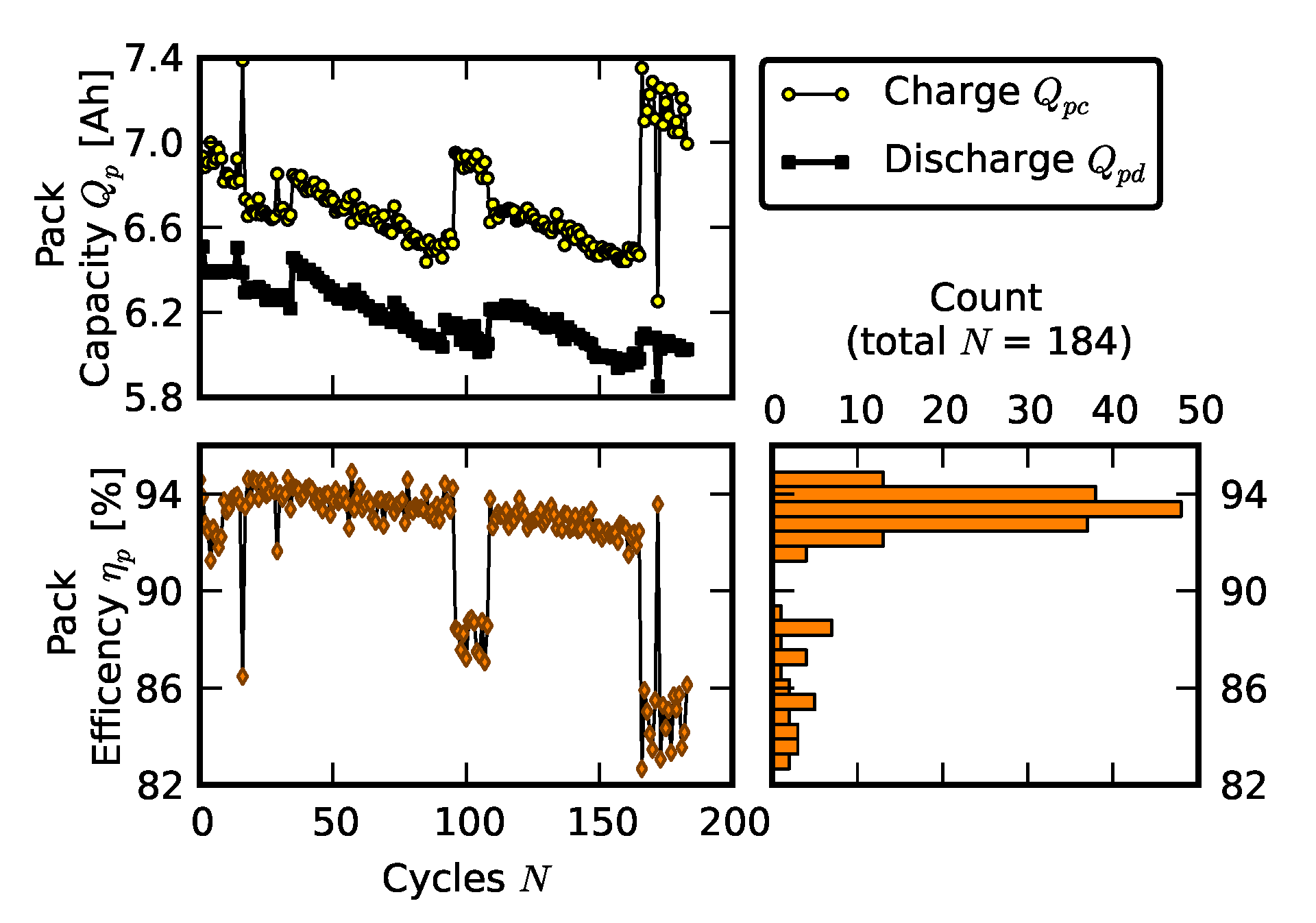
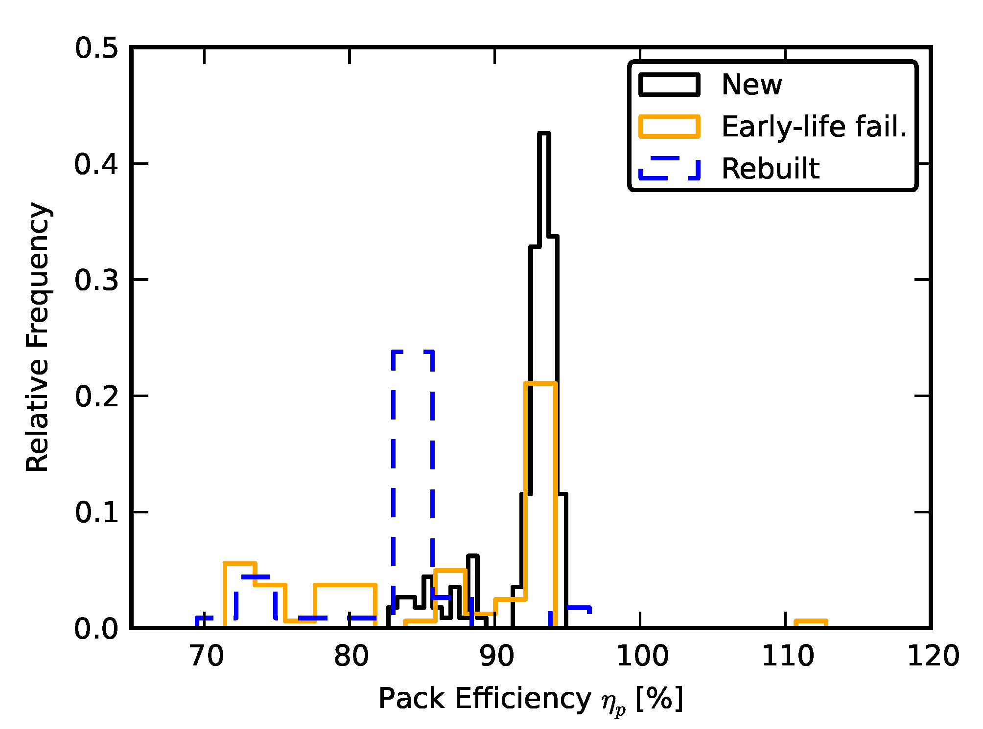
3.1. Efficiency Comparison

The pack performance is assessed with respect to its overall efficiency. Figure 11 shows a composite plot for pack efficiency. The top subplot shows the capacity at the end of discharge Q p d and capacity at the end of charge Q p c . Their ratio, pack coulombic efficiency η p , defined as
η = Q p d Q p c
and expressed in percent, is plotted on the bottom subplot. It is important to note that, while the pack was charged using constant current and constant voltage conditions, the discharge was conducted only in constant current condition. This approach is consistent with the single-cell charge-discharge profile and is reasonable from the pragmatic viewpoint of the user. The histogram of the efficiency is plotted in the right subplot in the horizontal direction, where the y-axis of the histogram is scaled to match the y-axis of the efficiency plot.
The main mode of the distribution of the coulombic efficiency of a pack comprised of all new cells is approximately 93%. As mentioned above, the pack cycling was interrupted periodically to take capacity measurements of individual cells and to record impedance spectra. Sometimes, after the test was resumed, the pack may have operated at somewhat different global capacity. This explains the occasional large step-shaped drops in efficiency. In addition to these abrupt drops, one can see that the overall efficiency degraded slowly, at approximately the same rate as the cell capacity. The efficiency of individual cells was about 99% on average (see Section 2.1, Figure 4c). The additional energy loss was attributed to cell balancing.
Figure 12 shows the efficiency of the pack built for Scenario 1 (early life failure study). Comparing this figure to Figure 11, it appears that the efficiency corresponding to the dominant mode of the distribution was very comparable to that of the pack comprised of new cells.
However, for the Scenario 1 pack, we observed more frequent abrupt drops in efficiency. One of the main indicators of cell aging is impedance increase [33]. Spectra of average impedance associated with the aged early life failure pack are displayed in Figure 13 in the usual way, with the x-axis being the real part of the impedance, R = { Z ̲ B a t t } , and the y-axis being the negative imaginary part of the impedance, Y = { Z ̲ B a t t } . Both R and Y are expressed in m Ω , with the frequency ranging from 10 mHz to 10 kHz. The plotted impedance traces are averages of nine individual-cell impedance measurements. There is a total of ten sets of measurements:
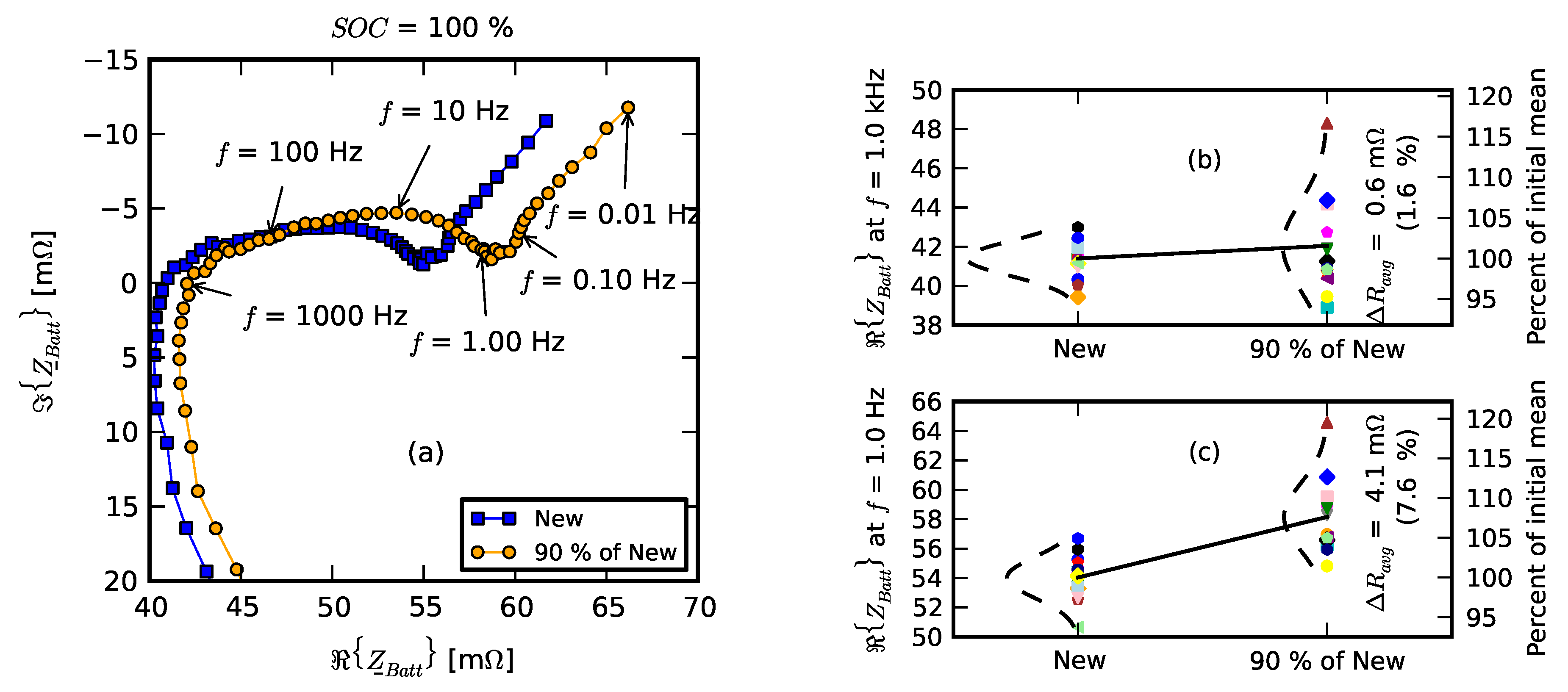
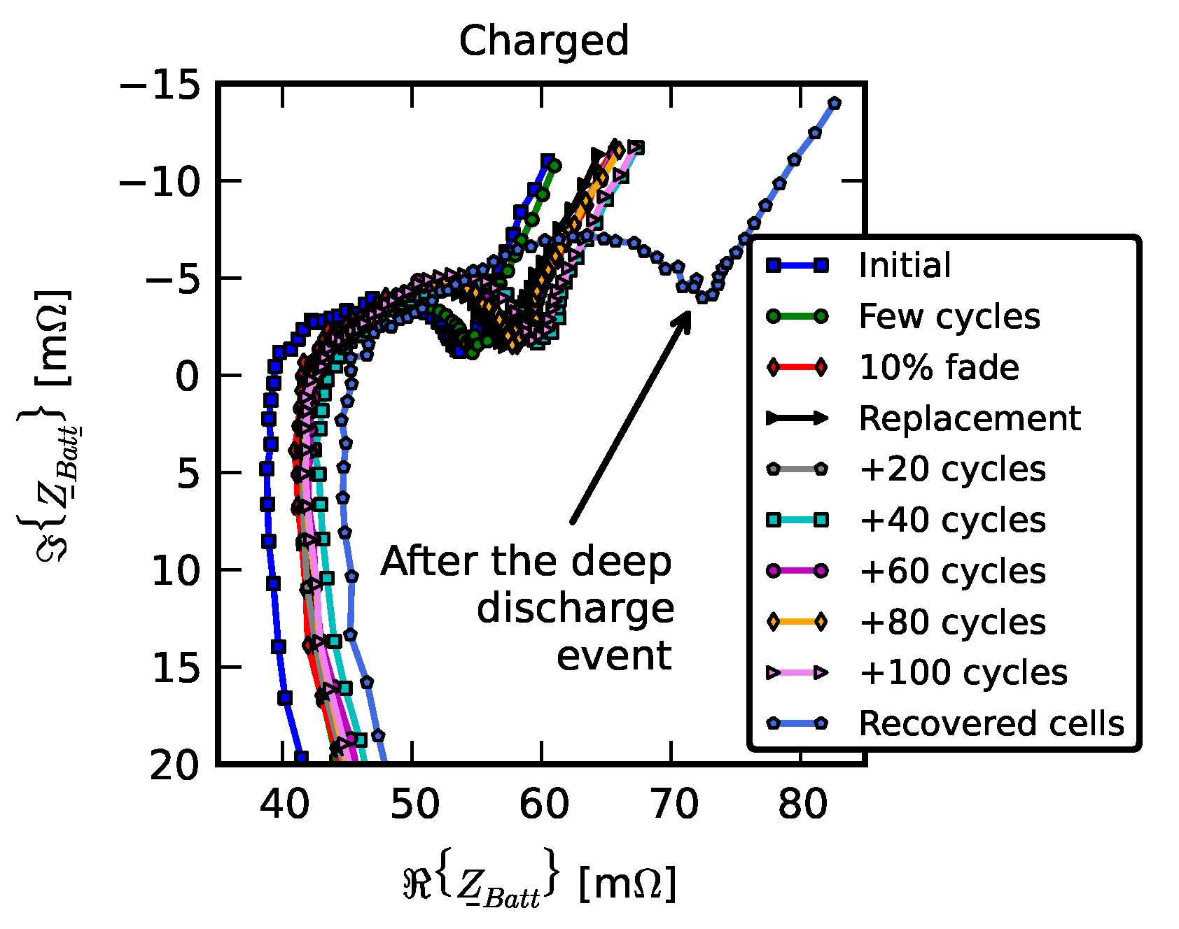
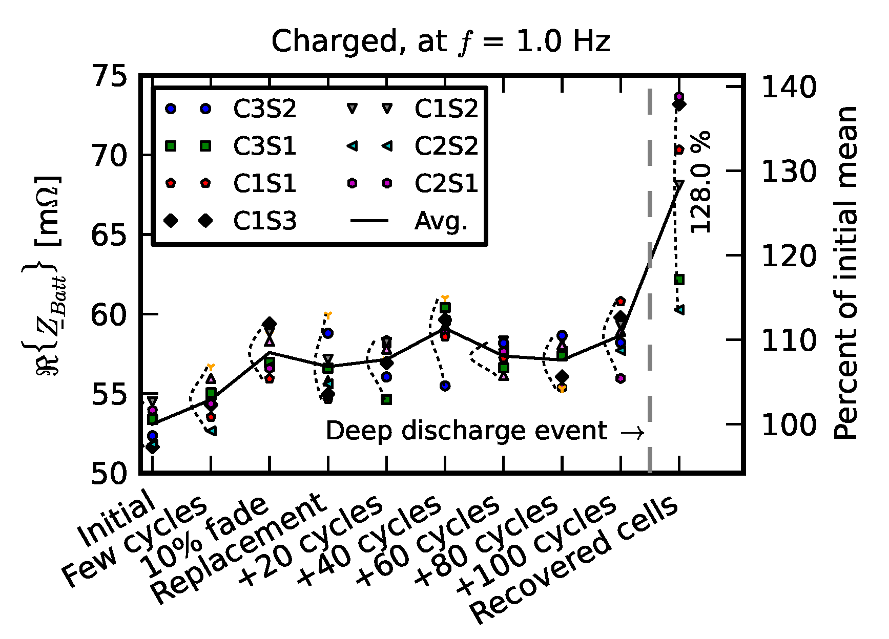
  • Initial signifies the measurements on new cells.
  • Few cycles signifies the impedance of nine cells after they were initially run in the pack for three cycles.
  • 10% fade signifies the measurements on the cell after they were individually aged on the single-cell tester to 90% of their nominal capacity.
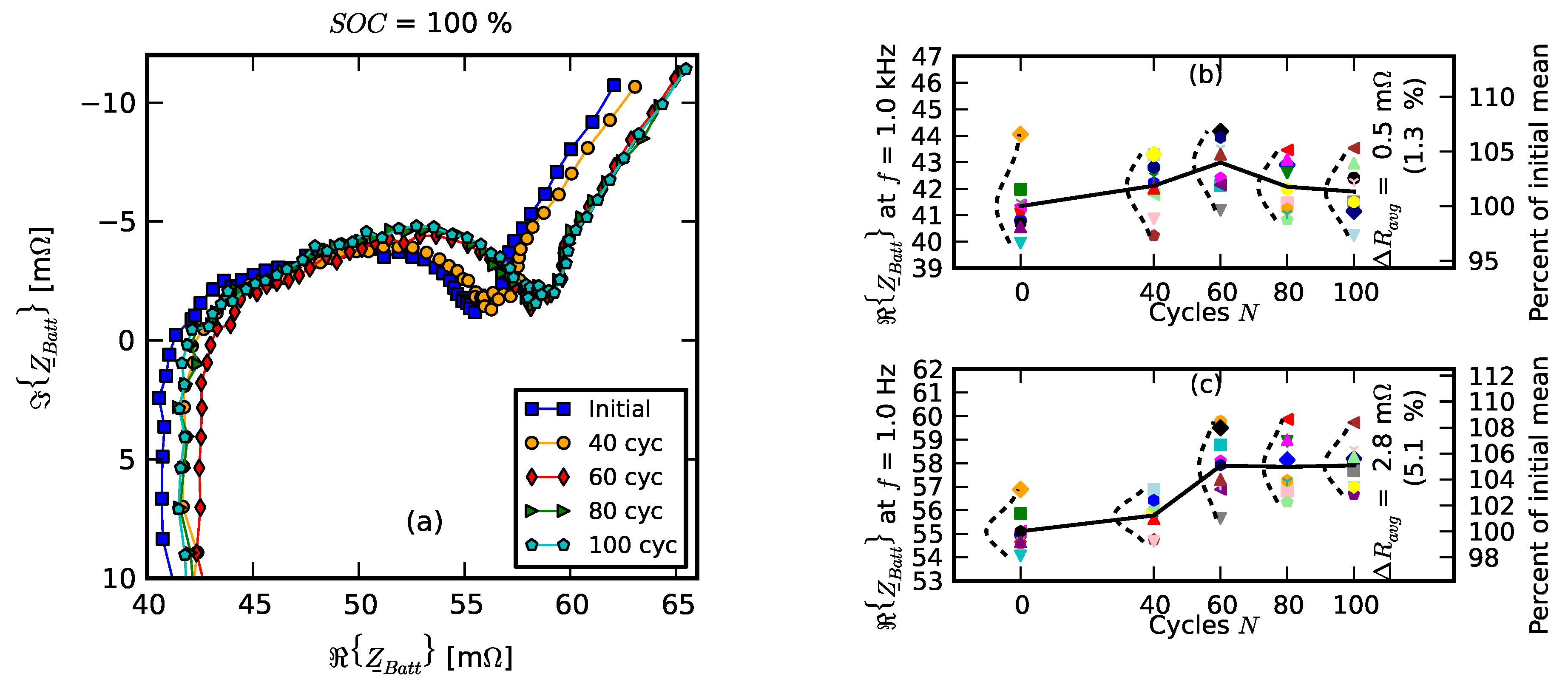
  • Replacement signifies resistance measurements after one cell was replaced with a new cell; +20 cycles, +40 cycles, +60 cycles, +80 cycles, and +100 cycles signify measurements as the “repaired” pack was operated for 100 cycles.
  • Recovered cells signify the impedance of a few cells that survived the deep discharge event.
At a high level, the shifts in the impedance spectra were larger initially. During the aging phase (+20 cycles through +100 cycles), the shifts were relatively small. Larger shifts occur at the points that correspond to lower frequencies. While R [ f = 1   kHz ] changed significantly after the deep discharge event on average, two of the six surviving cells were only moderately affected. This observation suggests that even after relatively violent failures, a subset of cells from a pack may retain nearly the same characteristics as before the failure.
Figure 14 shows distribution of the real part of the impedance measurements at f = 1 Hz. Here, the history of the testing is shown in the form of the x-axis tick marks. The measurements of individual cells are labeled with unique markers. Nine individual cell measurements correspond to each x-axis tick mark. The solid line connects the means of the nine cells, while the dashed curves represent the fitted normal distributions. While average resistance increased significantly after the deep discharge event, two cells were barely affected, as noted above.
The coulombic efficiency of the rebuilt pack (Scenario 2) is shown in Figure 15. This pack clearly operates at lower efficiency than the new pack (Figure 11) and the early life failure pack (Figure 12). Its dominant mode was at 85% efficiency. The reduced efficiency was due to larger mismatches among the comprising cells which required more balancing because passive cell balancing circuits dissipate imbalanced charge on a resistor. This result suggests that an active cell-balancing scheme may have potential for the pack based on repurposed cells because the return on the investment for these packs is faster. We return to this point at the end of the section.
Figure 16 compares the histograms of coulombicic efficiency of the three packs: the pack composed of new cells, the pack with an early failure, and the pack rebuilt from used cells. The dominant modes of the pack composed of new cells and the pack with an early failure largely overlap, and the dominant mode associated with the “rebuilt pack” is noticeably lower.

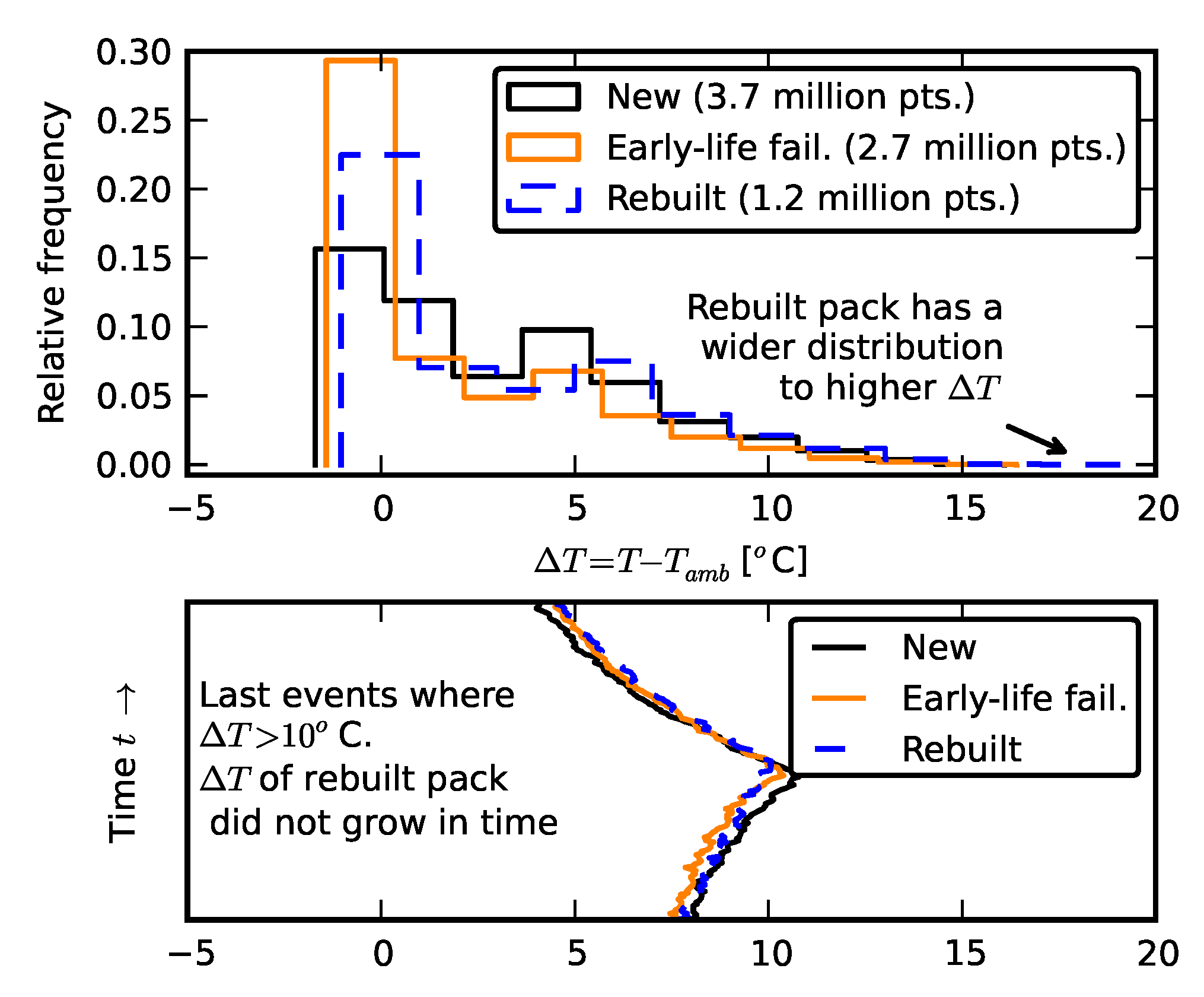
3.2. Temperature Effects

Local cell temperature variations and overall pack heating are important concerns in pack design. Within the confines of this study, we examined how temperature of individual cells increased during pack operation.
Figure 17 shows the distribution of temperature differences between individual cells and ambient temperature for the three packs. All test temperature measurements are included. There were no significant pack-to-pack differences in heating of individual cells, but the distribution of temperature differences of the rebuilt pack was slightly wider than the other two temperature distributions. The objective of the time domain plot on the bottom is to show that the “tail” of the distribution was not associated with the last cycles. The plot aligns the last event where Δ T exceeded 10 C for each of the three packs. The x-axis is temperature difference Δ T and was scaled to be the same as that of the histogram above; the y-axis is time. The peak corresponds to the end of discharge. The maximum Δ T of the bottom plot is considerably smaller than the maximum Δ T of the histogram. Thus, the tails of the histogram did not correspond to the aging, but to random variation. An alternative view of the data are provided in the Supplementary File.

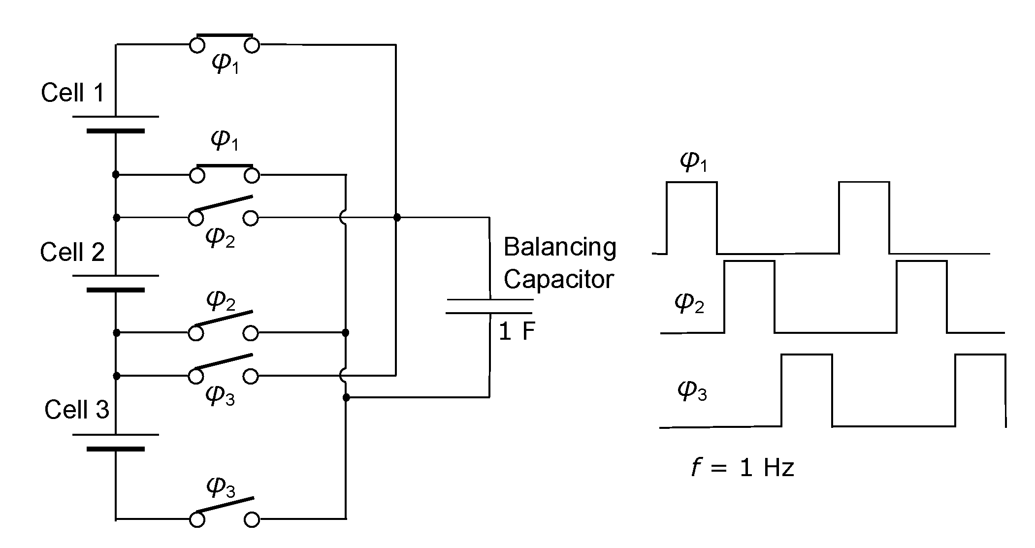
3.3. Effects of Balancing Scheme

As stated above, the mismatched cells required more balancing, and increased balancing directly translated into reduced efficiency. Some of the lost efficiency could be recovered by employing active cell balancing for the repurposed packs. To demonstrate this empirically, we created a pack consisting of a single string of three new serially connected cells and cycled this simple pack employing either passive or active balancing. The passive balancing scheme was the same as that employed for the test described Section 2.1, with the details provided in the Supplementary Materials.
The active balancing circuits employed a capacitor and solid state switches, as illustrated in Figure 18. The logic of the switches, denoted by symbols φ 1 φ 3 , connected only one of the cells in parallel with the capacitor. The cells took turns with respect to their connection to the capacitor in a circularly cyclical manner, as shown by the sketched waveforms of φ 1 φ 3 .
The data are shown in Figure 19a where total pack current waveforms are given in the top subplot and total charge associated with charge (bottom subplots) for a few charge/discharge cycles of the 3S1P pack while passive balancing scheme was used. The red and green colors were used to indicate charge and discharge cycles, while the blue color signifies the rest period. The efficiencies of individual cycles were denoted near the discharge points. The pack with passive cell balancing had 92.5% efficiency. Figure 19b shows the same information as Figure 19a when the pack employed active cell balancing.
The pack using the same cells and active balancing scheme had 96.6% efficiency, a 4.1% improvement over the passive balancing. In both cases, we ignored the first estimate because it would be based on a partial cycle. Because the average efficiency of new cells is almost 99.8% (see Section 2.1, Figure 4c), the improvement due to active balancing recovered more than half of the reduced efficiency, as illustrated in Figure 20.
The remaining losses were due to the equalization process which required additional current flows between the cells and the capacitor and the resistive imperfections of real solid-state switches (their on-state resistance), real equalizing capacitor (its equivalent series resistance), and the cells’ internal resistance. For example, during a charge cycle of an individual cell test, the current only flows into the cell, whereas during a charge cycle of the cell in a string, the current mostly flowed into the cell, but small amounts of current often flowed out of the cell during its connection to the capacitor. The balancing currents were completely dissipated if passive balancing circuit was used, and only partially dissipated in parasitic resistance of real circuit components in the active balancing circuit.

4. Conclusions

This study examined fundamental properties of aging lithium ion battery cells. We described the testing methodology and established that the cells in a carefully designed pack aged at the same rate as when they are individually aged. The careful design consisted of matching overall capacities of serial connections to minimize charge exchanges between strings and the associated dissipation, and also to match impedances within a serial connection to minimize equalization with its associated losses. We then considered two common scenarios in cell replacements: replacing a prematurely failed cell and building a new pack from cells of the damaged packs for less demanding applications. Less demanding applications considered here are those that can tolerate capacity of less than 70%. Stationary applications, e.g., microgrid storage, where the overall pack weight is not a limiting factor, are considered good examples of less demanding applications that can be source their cells and modules from high-demanding applications (e.g., transportation).
The first scenario is important for maintenance of existing packs and modules, especially large packs. We found that, at least for demanding applications where the pack operates until its cell drop to about 80% of the original capacity, a new cell coexisted well within a pack of aged cells. Therefore, within these applications, there may not be a need for a potentially expensive process of pre-aging cells.
The second scenario addressed the problem of repurposing of used cells in less demanding applications. To examine a severe case of a pack failure, we deeply discharged two packs and assembled a pack from the surviving cells. The deep discharge event was so severe that 6 of the original 18 cells were permanently damaged. Two approaches to rebuilding the packs were considered, but only matching the cells within a string worked robustly in our pack. After the pack was rebuilt in this fashion, more than forty cycles were successfully completed. Comparing the modes of the distribution, it was found that the overall pack efficiency of the rebuilt pack was about 8% lower than that of pack comprised of new cells. However, the heating of individual cells within the three packs was compared and no significant differences were found. We finally showed that increased losses due to larger mismatches can be partially compensated by employing active instead of passive cell balancing. The balancing scheme may be particularly critical for secondary applications where cells cannot be matched as well as in the primary applications, and where the initial mismatches are expected to grow further over time.
Lessons learned from this study will be employed in our future work of assessing opportunities for repurposing larger packs, where secondary applications may have specific use profiles distinctly different from the primary applications. For example, this information could be used in considering reuse of vehicle batteries in grid applications, such as peak shaving and smoothing of solar-generated power vs. their reuse in much smaller systems such as power tools, or toys. The future work may also consider other criteria, including economic and environmental performance.

Supplementary Materials

The following are available online at https://www.mdpi.com/2313-0105/6/3/39/s1, Figure S1: High-level view of the research program; Figure S2: Initial characterization and single-cell testing; Figure S3: Histogram of cell weights; Figure S4: Characteristic waveforms of a typical cycle; Figure S5:Impedance spectroscopy. (a) Average spectra. (b) Repeatability and potentiostat comparison; Figure S6: Schematic diagram of the 3S3P battery pack; Figure S7: (a) LabVIEW-controlled battery pack test stand. (b) Enlarged view of the pack; Figure S8:Voltage and current waveforms for a cell during pack cycling; Figure S9: Current distribution of three strings over four cycles; Figure S10:Voltage distribution of three cells within string 1 over four cycles; Figure S11: Cell balancing for one of the strings. Pack design employed 106 Astro "Blinky" from AstroFlight Inc. as the commercial cell balancer; Figure S12: Voltage distribution of three cells within string 1 over four cycles for active cell balancing; Figure S13:(a) Representative capacity of individual cells diverging in time (18650, lithium cobaltoxide chemistry). (b) Scatter plot of capacity fade vs. percent recovery; Figure S14: Capacity fade of eight lithium cobalt cells; Figure S15: Thermal image of the pack; Figure S16: Comparison of heating of lithium ion batteries; Table S1. Effect of T a on T e d ; Algorithm S1: Charge cycle.

Author Contributions

Conceptualization, N.G.N., T.A.T., and M.G.T.; methodology, N.G.N. and T.A.T.; software, N.G.N.; validation, N.G.N., T.A.T., and M.G.T.; formal analysis, N.G.N. and T.A.T.; investigation, N.G.N., T.A.T., and M.G.T.; data curation, N.G.N.; writing—original draft preparation, N.G.N.; writing—review and editing, N.G.N., T.A.T., and M.G.T.; visualization, N.G.N.; supervision, M.G.T.; project administration, M.G.T.; funding acquisition, M.G.T. All authors have read and agreed to the published version of the manuscript.

Funding

This work was made possible by the Office of Naval Research under Award No. N0004-07-1-0823.

Disclaimer

Any opinions, findings, and conclusions or recommendations expressed in this material are those of the author(s) and do not necessarily reflect the views of the Office of Naval Research.

Acknowledgments

We gratefully acknowledge the help of our colleagues from Rochester Institute of Technology: Scott Dewey for his assistance in pack assembly and instrument setup, Robert Kosty for his assistance in collecting data and debugging the fixtures, and Joseph Wodenscheck and Art Dee for skillful LabVIEW implementation of the charge cycle and discharge cycle on the battery pack test stand.

Conflicts of Interest

The authors declare no conflict of interest. The funders had no role in the design of the study; in the collection, analyses, or interpretation of data; in the writing of the manuscript, or in the decision to publish the results.

References

  1. Wagner, F.T.; Lakshmanan, B.; Mathias, M.F. Electrochemistry and the future of the automobile. J. Phys. Chem. Lett. 2010, 1, 2204–2219. [Google Scholar] [CrossRef]
  2. Williams, B.D.; Lipman, T.E. Strategy for Overcoming Cost Hurdles of Plug-In-Hybrid Battery in California. Transp. Res. Rec. J. Transp. Res. Board 2010, 2191, 59–66. [Google Scholar] [CrossRef] [Green Version]
  3. Ralston, M.; Nigro, N. Plug-in Electric Vehicles: Literature Review; Pew Center on Global Climate Change: Arlington, VA, USA, 2011; Available online: https://www.c2es.org/site/assets/uploads/2011/07/plug-in-electric-vehicles-literature-review.pdf (accessed on 22 July 2020).
  4. Witkin, J. A Second Life for the Electric Car Battery. 2011. Available online: https://green.blogs.nytimes.com/2011/04/27/a-second-life-for-the-electric-car-battery/ (accessed on 22 July 2020).
  5. Marano, V.; Onori, S.; Guezennec, Y.; Rizzoni, G.; Madella, N. Lithium-ion batteries life estimation for plug-in hybrid electric vehicles. In Proceedings of the 2009 IEEE Vehicle Power and Propulsion Conference, Dearborn, MI, USA, 7–10 September 2009; pp. 536–543. [Google Scholar] [CrossRef]
  6. Waag, W.; Fleischer, C.; Sauer, D.U. Critical review of the methods for monitoring of lithium-ion batteries in electric and hybrid vehicles. J. Power Sources 2014, 258, 321–339. [Google Scholar] [CrossRef]
  7. Rezvanizaniani, S.M.; Liu, Z.; Chen, Y.; Lee, J. Review and recent advances in battery health monitoring and prognostics technologies for electric vehicle (EV) safety and mobility. J. Power Sources 2014, 256, 110–124. [Google Scholar] [CrossRef]
  8. Lu, L.; Han, X.; Li, J.; Hua, J.; Ouyang, M. A review on the key issues for lithium-ion battery management in electric vehicles. J. Power Sources 2013, 226, 272–288. [Google Scholar] [CrossRef]
  9. Roscher, M.A.; Bohlen, O.S.; Sauer, D.U. Reliable state estimation of multicell lithium-ion battery systems. IEEE Trans. Energy Convers. 2011, 26, 737–743. [Google Scholar] [CrossRef]
  10. Kim, G.H.; Smith, K.; Ireland, J.; Pesaran, A. Fail-safe design for large capacity lithium-ion battery systems. J. Power Sources 2012, 210, 243–253. [Google Scholar] [CrossRef]
  11. Offer, G.J.; Yufit, V.; Howey, D.A.; Wu, B.; Brandon, N.P. Module design and fault diagnosis in electric vehicle batteries. J. Power Sources 2012, 206, 383–392. [Google Scholar] [CrossRef] [Green Version]
  12. Paul, S.; Diegelmann, C.; Kabza, H.; Tillmetz, W. Analysis of ageing inhomogeneities in lithium-ion battery systems. J. Power Sources 2013, 239, 642–650. [Google Scholar] [CrossRef]
  13. Zheng, Y.; Han, X.; Lu, L.; Li, J.; Ouyang, M. Lithium ion battery pack power fade fault identification based on Shannon entropy in electric vehicles. J. Power Sources 2013, 223, 136–146. [Google Scholar] [CrossRef]
  14. Li, J.; Barillas, J.K.; Guenther, C.; Danzer, M.A. Multicell state estimation using variation based sequential Monte Carlo filter for automotive battery packs. J. Power Sources 2015, 277, 95–103. [Google Scholar] [CrossRef]
  15. Dubarry, M.; Truchot, C.; Cugnet, M.; Liaw, B.Y.; Gering, K.; Sazhin, S.; Jamison, D.; Michelbacher, C. Evaluation of commercial lithium-ion cells based on composite positive electrode for plug-in hybrid electric vehicle applications. Part I: Initial characterizations. J. Power Sources 2011, 196, 10328–10335. [Google Scholar] [CrossRef]
  16. Dubarry, M.; Truchot, C.; Liaw, B.Y.; Gering, K.; Sazhin, S.; Jamison, D.; Michelbacher, C. Evaluation of commercial lithium-ion cells based on composite positive electrode for plug-in hybrid electric vehicle applications. Part II: Degradation mechanism under 2C cycle aging. J. Power Sources 2011, 196, 10336–10343. [Google Scholar] [CrossRef]
  17. Dubarry, M.; Vuillaume, N.; Liaw, B.Y. Origins and accommodation of cell variations in Li-ion battery pack modeling. Int. J. Energy Res. 2009, 34, 216–231. [Google Scholar] [CrossRef]
  18. Gering, K.L.; Sazhin, S.V.; Jamison, D.K.; Michelbacher, C.J.; Liaw, B.Y.; Dubarry, M.; Cugnet, M. Investigation of path dependence in commercial lithium-ion cells chosen for plug-in hybrid vehicle duty cycle protocols. J. Power Sources 2011, 196, 3395–3403. [Google Scholar] [CrossRef]
  19. Rao, Z.; Wang, S. A review of power battery thermal energy management. Renew. Sustain. Energy Rev. 2011, 15, 4554–4571. [Google Scholar] [CrossRef]
  20. Sarre, G.; Blanchard, P.; Broussely, M. Aging of lithium-ion batteries. J. Power Sources 2004, 127, 65–71. [Google Scholar] [CrossRef]
  21. Nenadic, N.G.; Bussey, H.E.; Ardis, P.A.; Thurston, M.G. Estimation of State-of-Charge and Capacity of Used Lithium-Ion Cells. Int. J. Progn. Health Manag. 2014, 5, 12. [Google Scholar]
  22. Dudek, K.; Lane, R. Synergy between electrified vehicle and community energy storage batteries and markets: Super session 4. Energy storage. In Proceedings of the Power and Energy Society General Meeting, Detroit, MI, USA, 24–28 July 2011; p. 1. [Google Scholar]
  23. Williams, D.M.; Gole, A.M.; Wachal, R.W. Repurposed battery for energy storage in applications of renewable energy for grid applications. In Proceedings of the 2011 24th Canadian Conference on Electrical and Computer Engineering (CCECE), Niagara Falls, ON, Canada, 8–11 May 2011; pp. 1446–1450. [Google Scholar]
  24. Schneider, E.L.; Kindlein, W., Jr.; Souza, S.; Malfatti, C.F. Assessment and reuse of secondary batteries cells. J. Power Sources 2009, 189, 1264–1269. [Google Scholar] [CrossRef]
  25. Lih, W.C.; Jieh-Hwang, Y.; Fa-Hwa, S.; Yu-Min, L. Second Use of Retired Lithium-ion Battery Packs from Electric Vehicles: Technological Challenges, Cost Analysis and Optimal Business Model. In Proceedings of the 2012 International Symposium on Computer, Consumer and Control (IS3C), Taichung, Taiwan, 4–6 June 2012; pp. 381–384. [Google Scholar] [CrossRef]
  26. Kamath, H. Lithium Ion Batteries in Utility Applications. In Proceedings of the 27th International Battery Seminar & Exhibit, Fort Lauderdale, FL, USA, 15–18 March 2010. [Google Scholar]
  27. Neubauer, J.; Pesaran, A.; Howell, D. Secondary Use of PHEV and EV Batteries: Opportunities & Challenges (Presentation); No. NREL/PR-540-48872; National Renewable Energy Lab (NREL): Golden, CO, USA, 2010. Available online: https://www.nrel.gov/docs/fy10osti/48872.pdf (accessed on 22 July 2020).
  28. Neubauer, J.; Pesaran, A. PHEV/EV Li-Ion Battery Second-Use Project; National Renewable Energy Laboratory: Golden, CO, USA, 2010. Available online: https://www.nrel.gov/docs/fy10osti/48018.pdf (accessed on 22 July 2020).
  29. Neubauer, J.; Pesaran, A.; Williams, B.; Ferry, M.; Eyer, J. Techno-Economic Analysis of PEV Battery Second Use: Repurposed-Battery Selling Price and Commercial and Industrial End-User Value; Report; National Renewable Energy Laboratory (NREL): Golden, CO, USA, 2012.
  30. Hawkins, J.M. Some field experience with battery impedance measurement as a useful maintenance tool. In Proceedings of the 16th International Telecommunications Energy Conference, INTELEC ’94, Vancouver, BC, Canada, 30 October–3 November 1994; pp. 263–269. [Google Scholar] [CrossRef]
  31. Lasia, A. Electrochemical impedance spectroscopy and its applications. Mod. Asp. Electrochem. 1999, 32, 143–248. [Google Scholar]
  32. Amine, K.; Chen, C.H.; Liu, J.; Hammond, M.; Jansen, A.; Dees, D.; Bloom, I.; Vissers, D.; Henriksen, G. Factors responsible for impedance rise in high power lithium ion batteries. J. Power Sources 2001, 97–98, 684–687. [Google Scholar] [CrossRef]
  33. Broussely, M.; Biensan, P.; Bonhomme, F.; Blanchard, P.; Herreyre, S.; Nechev, K.; Staniewicz, R.J. Main aging mechanisms in Li ion batteries. J. Power Sources 2005, 146, 90–96. [Google Scholar] [CrossRef]
  34. Dees, D.; Gunen, E.; Abraham, D.; Jansen, A.; Prakash, J. Alternating Current Impedance Electrochemical Modeling of Lithium-Ion Positive Electrodes. J. Electrochem. Soc. 2005, 152, A1409–A1417. [Google Scholar] [CrossRef]
  35. Tröltzsch, U.; Kanoun, O.; Tränkler, H.R. Characterizing aging effects of lithium ion batteries by impedance spectroscopy. Electrochim. Acta 2006, 51, 1664–1672. [Google Scholar] [CrossRef]
  36. Li, J.; Murphy, E.; Winnick, J.; Kohl, P.A. The effects of pulse charging on cycling characteristics of commercial lithium-ion batteries. J. Power Sources 2001, 102, 302–309. [Google Scholar] [CrossRef]
  37. Chen, M.; Rincon-Mora, G.A. Accurate electrical battery model capable of predicting runtime and IV performance. IEEE Trans. Energy Convers. 2006, 21, 504–511. [Google Scholar] [CrossRef]
  38. Saha, B.; Goebel, K. Uncertainty Management for Diagnostics and Prognostics of Batteries using Bayesian Techniques. In Proceedings of the 2008 IEEE Aerospace Conference, Big Sky, MT, USA, 1–8 March 2008; pp. 1–8. [Google Scholar]
  39. Shim, J.; Kostecki, R.; Richardson, T.; Song, X.; Striebel, K.A. Electrochemical analysis for cycle performance and capacity fading of a lithium-ion battery cycled at elevated temperature. J. Power Sources 2002, 112, 222–230. [Google Scholar] [CrossRef]
  40. Waag, W.; Käbitz, S.; Sauer, D.U. Experimental investigation of the lithium-ion battery impedance characteristic at various conditions and aging states and its influence on the application. Appl. Energy 2013, 102, 885–897. [Google Scholar] [CrossRef]
Figure 1. 3S3P pack (a) LabVIEW-controlled fixture; (b) enlarged view of the pack; (c) schematic.
Batteries 06 00039 g001
Figure 2. Waveforms associated with charge-discharge cycle (a) single-cell testing; (b) pack testing.
Batteries 06 00039 g002
Figure 3. (a) capacity fade (100–90%) as function of number of cycles; (b) capacity fade of nine cells within a pack over 100 cycles.
Batteries 06 00039 g003
Figure 4. (a) characteristic waveforms for a single cell: voltage V c , current I c , temperature T c , and ambient temperature T a ; (b) scatter plot of change in capacity at discharge in subsequent cycles Δ Q e d vs. temperature of the cell at the end of discharge Δ T ; (c) more details on capacity variation of a single cell over time.
Batteries 06 00039 g004
Figure 5. Impedance changes during single-cell aging. (a) average impedance spectra; (b) real part change for individual cells at f = 1 kHz; (c) real part change for individual cells at f = 1 Hz.
Batteries 06 00039 g005
Figure 6. Impedance changes during pack cell aging. (a) average impedance spectra; (b) real part change for individual cells at f = 1 kHz; (c) real part change for individual cells at f = 1 Hz.
Batteries 06 00039 g006
Figure 7. Individual capacities of the baseline pack comprised of new cells.
Batteries 06 00039 g007
Figure 8. Capacities of individual cells in an early life failure scenario where one cell C1S1 is replaced with a new cell after 10% capacity fade. Traces are labeled by the site of the cell in the pack.
Batteries 06 00039 g008
Figure 9. Capacities of individual cells in early life failure scenario.
Batteries 06 00039 g009
Figure 10. Equivalent circuit model (adapted from [37]).
Batteries 06 00039 g010
Figure 11. Coulombic efficiency of a pack during cycling (new cells).
Batteries 06 00039 g011
Figure 12. Coulombic efficiency of a pack during cycling (Scenario 1).
Batteries 06 00039 g012
Figure 13. Average impedance spectra of a pack comprised of eight aged cells and one new (Scenario 1).
Batteries 06 00039 g013
Figure 14. Real part of the impedance at f = 1 Hz at different stages of aging of early life failure pack (Scenario 1).
Batteries 06 00039 g014
Figure 15. Coulombic efficiency of a pack during cycling (Scenario 2).
Batteries 06 00039 g015
Figure 16. Overlaid coulombic efficiencies for the three packs.
Batteries 06 00039 g016
Figure 17. Comparison of heating of aging batteries.
Batteries 06 00039 g017
Figure 18. Circuit for active balancing of a 3S1P pack.
Batteries 06 00039 g018
Figure 19. Comparison of cell balancing for a 3S1P (a) passive; (b) active.
Batteries 06 00039 g019
Figure 20. Efficiency of passive balancing, active balancing, and individual cells.
Batteries 06 00039 g020
Table 1. Capacity of the recovered cells.
Cell IDCell Capacity Q c (Ah)
61.83
81.85
142.11
162.11
172.06
192.13
20max→ 2.14
212.12
231.73
241.69
25min → 1.58
272.02
μ 1.95
σ 0.20
Table 2. Resistances of the recovered cells.
Cell ID R f = 0.1 Hz (m Ω ) R f = 1 Hz (m Ω ) R f = 1 kHz (m Ω )
688.1877.9849.01
890.2480.41max→52.23
1464.8562.1244.00
1672.0770.0951.55
1772.4269.5550.27
1964.4761.7443.56
20min→62.61min→60.6444.74
2164.1561.5443.56
23max → 113.70max→86.66min→43.41
2499.3779.6449.14
25105.0283.7549.15
2769.9865.8145.65
μ 80.5971.6647.19
σ 17.969.563.36
Table 3. Cell and string capacities (in (Ah) for Option 1) that maximizes total pack capacity.
ConfigurationString 1String 2String 3
C 1 2.142.132.12
C 2 2.062.112.11
C 3 2.021.851.83
Total6.226.096.06
Table 4. Cell and string capacities (in (Ah) for Option 2) that best match capacity among the three strings.
ConfigurationString 1String 2String 3
C 1 1.832.112.06
C 2 1.852.121.73
C 3 1.851.582.02
Total5.815.815.81

