Abstract
Lithium (Li)-ion battery thermal management systems play an important role in electric vehicles because the performance and lifespan of the batteries are affected by the battery temperature. This study proposes a framework to establish equivalent circuit models (ECMs) that can reproduce the multi-physics phenomenon of Li-ion battery packs, which includes liquid cooling systems with a unified method. We also demonstrate its utility by establishing an ECM of the thermal management systems of the actual battery packs. Experiments simulating the liquid cooling of a battery pack are performed, and a three-dimensional (3D) model is established. The 3D model reproduces the heat generated by the battery and the heat transfer to the coolant. The results of the 3D model agree well with the experimental data. Further, the relationship between the flow rate and pressure drop or between the flow rate and heat transfer coefficients is predicted with the 3D model, and the data are used for the ECM, which is established using MATLAB Simulink. This investigation confirmed that the ECM’s accuracy is as high as the 3D model even though its computational costs are 96% lower than the 3D model.
1. Introduction
Recently, electric vehicles (EVs) have gained popularity as transportation vehicles [1,2]. Lithium ion (Li-ion) batteries are widely installed in EVs because of their high-power density, high energy density, long lifetime, and less self-discharge [1]. Since Li-ion batteries are usually utilized as main energy sources, management systems for batteries are essential for the development of EVs. In particular, battery thermal management systems (BTMSs) are important because the battery temperature during an operation affects the performance, lifespan, and safety of the batteries [1].
Many cooling methods are used for BTMSs, and the coolant materials can be mainly categorized into three types: air, liquid and phase change materials (PCMs). Air cooling is one of the most commonly used methods. Although it is simple and its advantage is the weight of the refrigerant, it is not suitable for a large capacity battery pack because air has a low thermal conductivity and heat capacity [3]. The PCM has a great advantage in terms of keeping the temperature of the batteries uniform or preventing thermal runaway. Nevertheless, for the long-term operation, the method is limited due to PCM full melting [4]. Liquid cooling is more efficient and compact, and it is widely used by several EV manufacturers, such as Tesla and General Motors (GM) [4]. Although water, mineral oil, or mixture ethylene glycol and water is adopted as the liquid coolant materials, the mixture of ethylene glycol and water is normally used by the EV manufacturers [1]. This is because the mixture has a lower melting point than 0 °C, and it is suitable for operating even in cold environments. Because the direct liquid cooling is concerned about the electrical short, indirect cooling using the thermal conductive media is often adopted. As with the media, tubes, cold plates with channels or jacket are used [1]. Since the heat pipe has a highly efficient thermal conductivity, BTMSs which adopt the heat pipe as the media are currently being studied. Nevertheless, there is room for improvement such as reducing the system complexity [3]. In this work, since it is intended for general-purpose modeling, we will target the BTMS of the liquid cooling using a mixture of ethylene glycol and water, which is often used in popular EVs.
Numerical simulations are useful for predicting and evaluating the impact when varying the design, and they are expected to reduce the study period and cost. Numerical simulations are used in many reports for BTMSs, and the method can be categorized into two types: detailed models and equivalent circuit models (ECMs). Detailed models [5,6,7,8,9,10,11,12,13] usually target two-dimensional (2D) or three-dimensional (3D) thermal phenomena in battery cells or modules with finite element methods (FEMs) or finite volume methods (FVMs). Y. Chung et al. [5] performed a thermal analysis with a 3D model to improve the cooling design of pouch battery packs. Siruvuri et al. [6] also modeled a battery pack and the cooling channels and optimized the design to reduce the peak temperature by reversing the direction of the water flow in one of the channels. Although these detailed models have merits for grasping the mechanism and predicting the results more reliably, these are not suitable for predicting the large-scale phenomenon such as the whole battery pack because the computational costs are higher.
Because ECMs [3,4,14,15,16,17] have low computational costs, these models can be adopted for the whole battery pack and for controlling the interaction among multiple parts with electronic control units (ECUs) during the drive operation. The developed ECMs are useful considering the development of all the BTMSs installed in the ECUs. By having a uniform environment, some programs, such as MATLAB Simulink® (Natick, MA, USA), can be useful for establishing the ECMs. Y. Gan et al. [3] developed a thermal ECM for the heat pipe-based thermal management system for a battery module, and they validated the model with experimental data. M. Shen et al. [4] constructed a system simulation model by using a refrigerant-based battery thermal management system, and they improved the system’s performance.
Since ECMs have more abstract modeling, it is more difficult to confirm intuitively that the model assumption is satisfied with the target phenomenon. In most reports for ECMs, some important parameters that are represented by the heat transfer coefficients or the pressure drops are determined with some theoretical equations. However, the structural design of the flow channels has become more complex, to improve the efficiency. In addition, it may not be clear that conventional theoretical equations can be generally adopted for the flow in channels. Moreover, because these equations sometimes have a range of applicable values or fitting parameters when taking into account the various impacts, such as geometric factors, the model design is more complex, and it may cause the model to contain potential mistakes.
In this study, we propose a framework in which the ECMs can be established with a unified method by using detailed 3D models. We also present a model for the thermal–electrical coupled ECM of the liquid cooling phenomenon for the battery pack, which includes the experimental methods, and the model is validated with experimental data.
2. Methodology for the Test Bench and the Detailed 3D Model
2.1. Electrical ECM Modeling with the Experimental Data
The battery pack for the liquid cooling experiment is constructed with five commercial Li-ion battery modules in which two pouch-type Li polymer cells are connected in series. The cell size is 36 mm × 125 mm × 6.5 mm. In this study, it is defined that the open-circuit voltage (OCV) of a cell is 3.0 V when the state of charge (SOC) is 0%, and the OCV of a cell is 4.2 V when the SOC is 100%. In addition, it is confirmed that the charging and discharging capacities are 3.0 Ah in the OCV range between 6.0 and 8.4 V for the module.
The experiment to evaluate the discharge properties of a module was performed based on the following procedures:
- (i)
- Keeping the module at a set environmental temperature in the thermostatic chamber.
- (ii)
- Charging the module following the constant current (CC)-the constant voltage (CV) procedure to 8.4 V with a 0.2C current rate.
- (iii)
- Rest period of 60 min.
- (iv)
- Discharging the module following the CC procedure with a set current rate until the SOC decreases by 10%.
- (v)
- Rest period of 60 min.
- (vi)
- Performing operations (iv) and (v) until the cell voltage reaches 6.0 V.
The combinations of the environmental temperature and current rate are shown in Table 1. The experiment for the charge properties was also performed with similar procedures. Then, the temporal behavior of the electrical potential per SOC 10% during the intermittent discharge or the charge under each condition were obtained, respectively. In the model, the SOC is calculated as follows.
where SOC0 is the initial state of the charge; t is the time; Cc is the capacity, which is equal to 3 Ah; and I is the electric current, in which a positive value represents the charge and a negative value indicates a discharge.

Table 1.
The combinations of the experimental condition in order to evaluate the battery module’s charge and discharge properties.
For the electrical ECM for the batteries, the model shown in Figure 1a is adopted. The internal resistance is calculated from the experimental data as follows.
where R is the internal resistance per cell, V is the voltage per cell, and OCV is the open-circuit voltage. Because two cells in the module are assumed to be in the same state, V is half of the module voltage. Further, OCV is calculated by the cubic Hermitian interpolation polynomial with the voltage immediately before the CC discharge during the discharge experiment, as shown in Figure 2n.
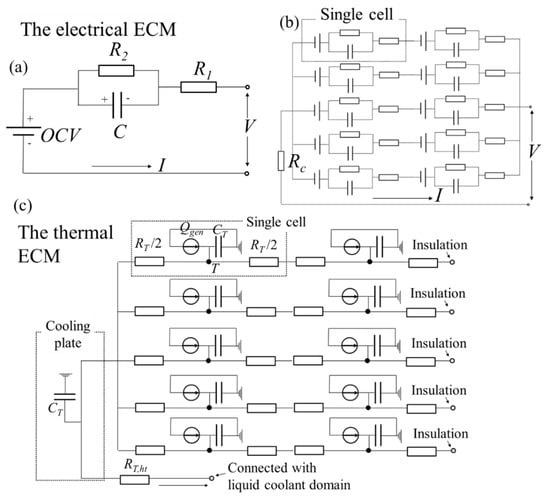
Figure 1.
The schematic views of (a) the electrical equivalent circuit model (ECM) for a single cell, (b) the electrical ECM for the whole battery pack, and (c) the thermal ECM for the whole battery pack.
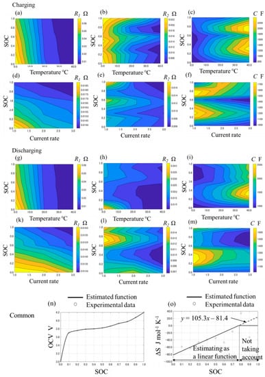
Figure 2.
The relationship between the variable parameters and the arguments in the electrical ECM. (a–f) show the relationship between R1, R2, C and temperature, current, state of change (SOC) at charge, (g–m) show it at discharge, (n) shows the relationship between SOC and open-circuit voltage (OCV), and (o) shows the relationship between SOC and ΔS.
In the electrical ECM, the internal resistance during the CC charge or discharge is calculated theoretically as follows.
where t’ is the time after the charge or discharge, and R1, R2, and C are the resistance or capacitance components as shown in Figure 1a. R1, R2, and C are assumed be dependent on the temperature, current, and SOC, and they are optimized by fitting these parameters for the experimental data, which is calculated by applying Equation (2). The values of R1, R2, and C can be calculated by applying a linear interpolation or extrapolation with the database of the relationship between these parameters and the temperature, current, and SOC. The contours of the relationship are indicated in Figure 2a–m. From these figures, it is considered that the resistance R1 and R2 have a negative correlation with the temperature. This is because the electrochemical reaction degree and the Li-ion conductivity increase with a higher temperature. It is also considered that R1 and R2 have a negative correlation with the current rate. This is because the nonlinear relationship between the current and overpotential is indicated with the Butler–Volmer equation.
The heat generation of batteries is calculated by the following formula.
where: Qgen is the total heat generation, Qirr is the irreversible heat generation due to the heat from the internal resistance, Qrev is the reversible heat generation due to the entropy change, T is the temperature, is the entropy change, and F is the Faraday constant. By applying Equation (4), the entropy change is calculated by and the results are shown in Figure 2o as the plot points. The data of the entropy change almost monotonically increases with the SOC, and the tendency and values are similar to the batteries that consist of the LiCoO2 cathode and the graphite anode [18,19]. However, the values from SOC = 50% to SOC 80% vary strongly, and the tendency is different from the measurement in some reports [18,19]. We estimate that the tendency is affected by the measurement error because of the lack of experimental data. In this model, from the perspective that simple modeling is preferred, a linear regression is adopted for the entropy change when the SOC is less than 80% with the least squares methods. In addition, the entropy change when the SOC is more than 80% is not taken into account, which is illustrated in Figure 2o.
2.2. Testing of the Liquid Cooling for a Battery Pack
The schematic view of the test bench is shown in Figure 3. The test bench is constructed roughly with five battery modules, a cooling plate, some tubes for the flow channels, and a chiller. Although the constitution of the test bench is simpler than the actual systems for the EVs, we consider that the test bench has roughly the same component as the actual systems, and it is sufficient to explain the usefulness for our framework. Five battery modules are connected in parallel, and the terminals are connected with the device for the battery management and the direct current (DC) power supply. We defined these batteries as a battery pack whose capacity is 15 Ah, and its operating voltage is from 6.0 V to 8.4 V. These modules are set on the cooling plate, which has a meandering flow channel. Liquid coolant is circulated among the chiller and the flow channel via the tubes, and the temperature of the liquid coolant in the chiller is maintained at 25 °C. As the liquid coolant, we adopt long life coolant, which is mainly a mixture of ethylene glycol and water. The batteries and cooling plate are covered with heat insulators in order to reduce the impact of the heat transfer from other than the liquid coolant. Therefore, most of the heat radiation is due to the outflow of the liquid coolant. The battery pack is pressed down at about 100 Pa to reduce the impact on the contact resistance between the batteries and the cooling plate. The temperature for the top of the battery modules and the liquid coolant flowing in the tubes is measured by using thermocouples. The volume flow rate of the liquid coolant through the cooling plate flow channel is measured with an electromagnetic flow meter.
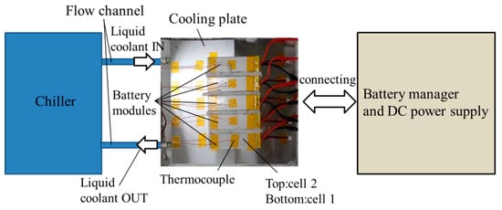
Figure 3.
The schematic view of the test bench.
The charging and discharging for the battery pack were performed with the following procedures:
- (i)
- Discharging of the battery following the CC-CV procedure to 6.0 V with the 0.2C current rate.
- (ii)
- Rest period of 60 min.
- (iii)
- Charging the battery to 8.4 V with a 2C current rate.
- (iv)
- Discharging the battery to 6.0 V with a 2C current rate.
- (v)
- Performing two cycles of operations (iii) and (iv).
The tests are performed twice under conditions for the chiller setting in which the flow rate is 0.0 l·min−1, i.e., not flowing, or 1.0 l·min−1. In this work, the case of not flowing is called case 1, and the case of 1.0 l·min−1 is called case 2.
2.3. Constructing the Detailed 3D Model
The detailed 3D model for the tests was developed. The overview of the calculation meshes and the geometry of the flow channel in the cooling plate are illustrated in Figure 4. The shapes are modeled by measuring the actual things. The prism meshes are adopted into the flow channel close to the wall of the cooling plate. In addition, they have two layers whose thickness is less than 1 mm to resolve the temperature boundary layers. The others are the tetrahedral meshes, and the total number of elements is 992,623. It is confirmed that the calculation results did not vary with more refined meshes. For the same reason, the relative tolerance of the progress for the next time step is set as 1.0 × 10⁻³.
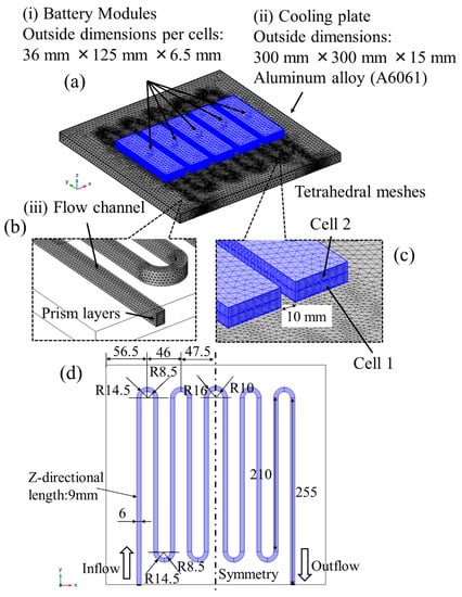
Figure 4.
The overview of the calculational meshes and the geometry of the flow channel in the cooling plate. (a) shows the whole overview of the calculational meshes, (b,c) show the detail view of the flow channel and the cells, and (d) shows the geometry of the flow channel in the cooling plate.
The flow field and pressure field in the liquid coolant domain are presented as the equations of the mass continuity and the Navier–Stokes equations for incompressible flow, which are described as follows.
where u is the flow velocity vector, ρ is the density, p is the pressure, I is the identity matrix, and μ is the kinematic viscosity. In this model, the flow is assumed to be a steady laminar flow because the Reynolds number is low when the flow rate is less than 1.0 l/min. The heat transfer phenomenon in the whole domain is presented as the heat transfer equation, which is described below.
where Cp is the specific heat at a constant pressure, k is the thermal conductivity vector, and VL is the volume of a cell. The flow velocity vector u in the liquid coolant domain can have a value other than 0, and u = 0 in the other domain. Qgen in the domains other than the batteries is 0. In this model, the heat generation is assumed to be uniform per the battery cell, and the electrical ECM is shown in Figure 1b, which is calculated per time-step to evaluate Qgen in Equation (4). Note that the symbol Rc is the electrical contact resistance due to the connection of the conductors, and it is estimated to be 7.8 mΩ. The thermal contact resistance between the cooling plate and the liquid coolant is not taken into account because pressing the battery pack is supposed to reduce it sufficiently. This system of equations is discretized by the FEM and it is solved by using initial and boundary conditions. These numerical calculations are conducted by using COMSOL Multiphysics® ver. 5.4. Table 2 lists the physical properties that use this model.
Table 2.
The physical properties using the simulations. Superscript “a” indicates the assumed value.
The charging or discharging conditions for the battery pack are the same as the experiment. For the inlet boundary of the liquid coolant domain, the flow rate is 0.0 l·min−1 and the temperature is 23.5 °C under case 1. Meanwhile, the flow rate is 0.862 l·min−1 and the temperature is 25.2 °C under case 2. These values are given by averaging the measured data. The pressure is set as 0 Pa for the outlet boundary under case 2. Under case 1, the outlet boundary condition is assumed to be the same as the inlet boundary condition. The outside boundaries except the flow outlet are insulated thermally.
The assumptions made for the model are as follows.
- (1)
- The flow of the liquid coolant is assumed to be a steady laminar flow. Therefore, the turbulence models are not adopted.
- (2)
- The heat generation is assumed to be uniform per the battery cell.
- (3)
- The inlet flow conditions are set by the measured data.
- (4)
- If there is no flow, the outlet boundary condition is assumed to be the same as the inlet boundary condition.
- (5)
- The heat loss to the outside is not taken into account except due to the flow outlet.
2.4. The Thermal–Electrical Coupled ECM
The thermal ECM for the battery pack cooling system was constructed based on the detailed 3D model. The schematic view is presented in Figure 1c. The thermal resistance, heat capacities, and heat generation are linked within the ECM. The temperature of each component, except for the liquid coolant domain, is calculated by the energy balance equation.
where CT is the heat capacity that is calculated by ρCpVL, and Qlink is the heat transfer into or from the linked components, which can be determined from Equation (9).
where RT is the thermal resistance, and is the temperature difference between the target component and the linked components. In the liquid coolant domain, the temperature can be determined by applying Equation (10).
where Qht is the heat transfer that is exchanged between the cooling plate and the liquid coolant domain, Qf is the heat due to the liquid coolant flow through the flow channel, RT,ht presents the liquid–solid heat transfer as the thermal resistance, is the mass flow rate, and is the liquid temperature difference between the inlet and the outlet. RT,ht is described as follows.
where h is the heat transfer coefficient, and A is the liquid–solid cross-sectional area.
From the 3D model’s result, the temperature distribution in the cells has a large gradient in the z-direction and it is in the cooling plate, which is not large. Therefore, z-directional thermal links are taken into account for the cell, and one component is taken into account for the cooling plate. The parameter values are calculated from Table 2 and the geometry of the 3D model. For example, the cell thermal resistance RT is calculated by lT/(AT kz) where lT is the length of the heat pass, AT is the cross-sectional area, and kz is the z-directional thermal conductivity. The thermal–electrical coupled ECM is constructed by using MATLAB Simulink® R2019a/Simscape, and the schematic views are illustrated in Figure 5.
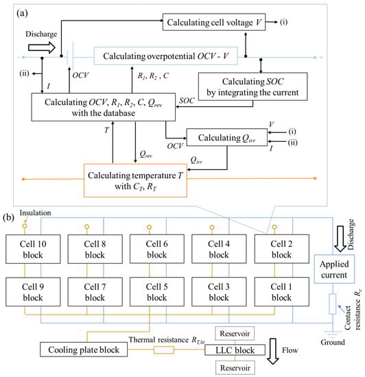
Figure 5.
The schematic views of the electrical-thermal coupled ECM for (a) the single cell and (b) the whole battery pack. Note that the blue lines indicate the electrical links and the orange lines indicate the thermal links.
The heat transfer coefficient h is estimated by the results of the 3D model. The calculations are performed with the above 3D model, in which the uniform temperature of 26 °C was set to the liquid–solid cross-sectional boundary. The flow and temperature field were calculated only for the liquid coolant domain. Further, the temperature on the inlet boundary is 25 °C and the results are given under the various flow rate conditions where the range of the flow rate is from 0 l/min to 1 l/min. The heat transfer coefficient can be determined as follows.
where qn is the normal directional heat flux on the liquid–solid cross-section; Ts is the solid temperature, which is equal to 26 °C; and is the inlet liquid temperature, which is equal to 25 °C. In the ECM, the values that were calculated by the cubic Hermitian interpolation polynomial are adopted.
3. Results and Discussion
3.1. The Test Bench and the 3D Detail Model
The temperature distributions after 300 s and 2700 s under case 2 are shown in Figure 6. Large temperature gradients in the Z direction in the cells are confirmed after 300 s and 2700 s although the temperature gradients in the X and Y direction are small. Moreover, after 300 s, the temperature in the cells is lower than the cooling plate because of the endothermic reactions of the entropy change during charging. On the other hand, after 2700 s, the temperature in the cells is higher, and it reaches approximately 36 °C because of heat generation from the Joule heat and the exothermic reactions of the entropy change during discharge. The temperature for the outflow is approximately 0.5 °C higher than the inflow. The time histories of the total voltage and temperature for cases 1 and 2 are shown in Figure 7. From Figure 7a,c, under both cases, the voltage of the battery pack increases from 6.0 to 8.4 V during charging, and it decreases from 8.4 to 6.0 V during discharging. It is confirmed that the values agree with the experimental data. From Figure 7b,d, the temperature on the surface of cell 2 decreases immediately after the starting charge because of the endothermic reactions, and it increases significantly after it starts charging again. The difference between case 1 (without flow) and case 2 (with flow) per cycle is smaller than the temperature rise and drop due to the heat generation or the endothermic reactions because the applied current is high rate (2C). The temperature drop under case 1 is considered to be mainly due to the endothermic reactions and heat transfer to the cooling plate which has high heat capacity and high thermal conductivity. In the experimental data of the first cycle, the total temperature rise on the surface of cell 2 is 11.6 °C (initial: 23.9 °C, and final: 35.5 °C) under case 1 and 10.1 °C (initial: 24.9 °C, and final: 35.0 °C) under case 2. Therefore, approximately 1.5 °C is the impact of the flow. Especially when the temperature becomes high, the difference between the 3D model and the measured data increases slightly, and the maximum error is approximately 2 °C. This is mainly because heat dissipation, such as the heat flow via air or the pipes that are connected with the cooling plate, is not taken into account in the 3D model. In this work, because the set flow rate is relatively low, the heat paths other than the liquid cooling are not sufficiently small to ignore its effects. Nevertheless, the values during charging agree well with the measured data, and the difference does not increase per cycle under the two experimental conditions. In addition, the heat capacities and heat generation are supposed to be valid. From Figure 7e, the tendency of the temperature at the outlet agrees with the experimental data. This fact indicates that the heat dissipation due to the liquid coolant flow is similar between the 3D model and the experiment. From the above, it can be determined that the 3D model is validated sufficiently with the experiment.
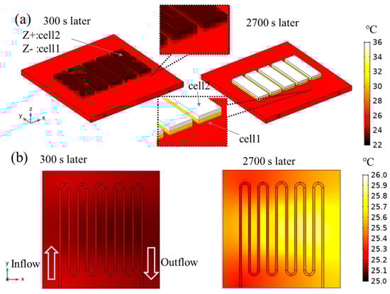
Figure 6.
(a) The temperature distributions on the surfaces and (b) it in the z-directional center cross-section of the flow channel after 300 s and 2700 s in the 3D model under case 2.
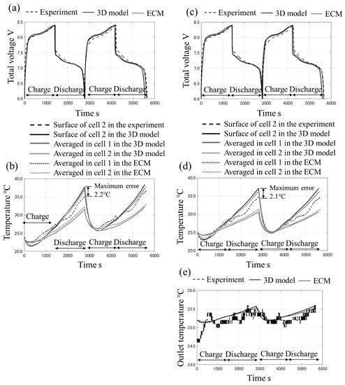
Figure 7.
The time histories of the total voltage under (a) case 1 and (c) case 2, the time histories of averaged temperature and surface temperature under (b) case 1 and (d) case 2, and (e) the time histories of outlet temperature.
Under case 2, the calculation time of the model is 140 min performed by using two Intel® Xeon® CPU E5-2699 v3 @ 2.30 GHz processors with a memory of 128 GB, and the calculation cost may not be small enough. Therefore, it may need more effort or more powerful computational power to calculate a huge scale phenomenon such as battery packs with tens of battery cells, which is often installed for EVs.
3.2. The Thermal–Electrical Coupled ECM
According to Figure 7, it is clear that the results of the ECM agree well with the 3D model. From this, the ECM is supposed to be a surrogate model for the 3D model because the heat coefficient is determined with its data and the links of the thermal ECM are also determined based on its temperature distribution results. Table 3 shows the summary of computational environment and calculation costs of our models. Under case 2, the calculation time of the ECM is 5.0 min, which is 96% lower than the 140 min of the 3D model.
Table 3.
Computational environment and calculation costs of our models.
In the ECM, the value calculated by the 3D detail model is adopted as the liquid–solid heat transfer coefficient, shown in Figure 8a. In comparison, the parameters are also calculated by applying conventional theoretical equations. The heat transfer coefficient can be determined by applying Equation (13).
where kf is the liquid thermal conductivity, Dh is the hydraulic diameter of the flow channel, and Nu is the Nusselt number, which is known to be constant if the flow is a fully developed laminar flow in a straight flow channel and the heat fluxes or temperature are uniform [21]. As demonstrated in the literature [21], if the duct is a rectangular cross-section and the temperature is uniform, Nu is 3.08 when the aspect ratio is 1.43, and Nu is 3.39 when the aspect ratio is 2.0. The aspect ratio of the flow channel is 1.5, and Nu is 3.12 based on linear interpolation. According to Figure 8a, the results of the 3D model increase linearly with the flow rate, and the tendency is different from the above theoretical results. When the flow rate is less than 0.2 l·min−1, the heat transfer coefficient is less than the line where Nu = 3.12. This is because the prerequisite of the above theoretical equation is not satisfied. It is assumed that the axial conduction can be negligible [21] under the conditions where the heat diffusion into the inlet boundary is the main phenomenon and the axial conduction is not negligible. When the flow rate is more than 0.2 l·min−1, there is an increase in the flow rate. This is because the heat exchange efficiency is higher than a straight flow channel due to the flow bias as shown in Figure 8d. More consideration for this effect is described in Appendix A in detail.
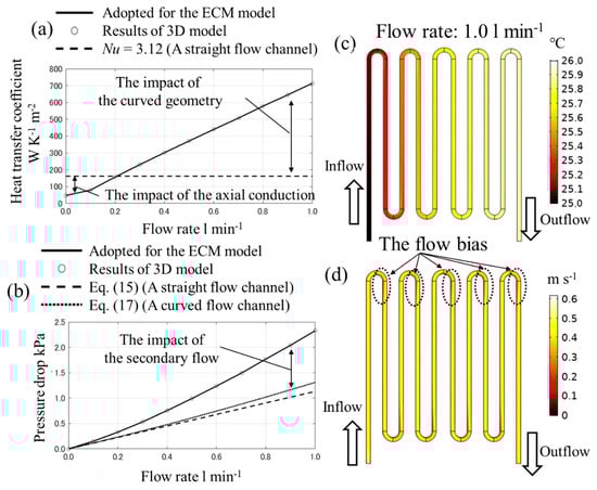
Figure 8.
The relationship (a) between the flow rate and the heat transfer coefficient, (b) it between the flow rate and the pressure drop, (c) the temperature distribution and (d) the velocity magnitude distribution in the z-directional center cross-section of the flow channel when the flow rate is 1.0 l·min−1.
The pressure drop Δp in the 3D model can be calculated as follows.
where is the mean pressure in the inlet boundary, and is the mean pressure in the outlet boundary. The pressure drop in a straight flow channel can be theoretically calculated by applying the Darcy–Weisbach equation as demonstrated in Equation (15).
where L is the total length of the flow channel, f is the Darcy friction factor, and um is the cross-sectional mean flow velocity in the flow channel. There are formulations to calculate f, which have been proposed by S.W. Churchill [22] and V. Bellos et al. [23] and so on. Nevertheless, if only laminar flow is considered, the Darcy friction factor f can be calculated as follows [24,25].
where Re is the Reynolds number. Moreover, the impact of the curved geometry of the flow channel can be taken into account by applying Equation (17) [24,25].
where Kb is the bend loss coefficient, which is dependent on the bend angle and the ratio between the bend radius and the hydraulic diameter. By having a bending angle of 180 degrees [24], Kb = 0.413 when the bend radius is 11.5 mm and Kb = 0.401 when the bend radius is 13.0 mm.
According to Figure 8b, it is confirmed that the gradient of the 3D model is higher by applying Equations (15) and (17). This is because of the secondary flow’s difference between the rectangular cross-section and the circular cross-section. Note that the evaluation for Kb is performed based on the circular cross-section flow. In the rectangular cross-section, the corner obstructs the secondary flow and it may increase the pressure loss.
It needs to be emphasized that the theoretical equations can be modified to take into account the presented impacts and it is adopted for the ECM. Nevertheless, in our framework, these processes are not necessary except for the validation of the 3D model, and the modeling consideration may become simpler. Although only laminar flow model is used in this demonstration for our framework, the turbulence model can be adopted for the 3D models.
4. Conclusions
In this study, we describe a framework in which a thermal–electrical coupled ECM for a cooling system of a battery pack is constructed with a detailed 3D model. It is confirmed that the ECM has the same accuracy as the 3D model, which is validated through experimental results. The conclusions are described as follows:
- (1)
- To match the ECM’s results with the 3D model, the liquid–solid heat transfer coefficient and the links of the thermal ECM are determined with the 3D model’s results.
- (2)
- The ECM’s accuracy is as high as the 3D model even though its computational costs are 96% lower than the 3D model.
- (3)
- In terms of the 3D model’s disadvantages, there may be a cost for constructing and validating the 3D model, and it may need more effort or more powerful computational power to calculate a huge scale phenomenon such as battery packs with tens of battery cells, which are often installed for EVs.
- (4)
- The tendency of the liquid–solid heat transfer coefficient and the pressure drop do not agree well with the 3D results and some theoretical equations, since this phenomenon does not satisfy some prerequisites for the theoretical equations. Although theoretical equations can be determined and adopted for the ECM, the 3D model is advantageous because of its simplicity and certainty.
Author Contributions
Conceptualization, T.Y. (Takumi Yamanaka) and T.Y. (Tatsuya Yamaue); methodology, T.Y. (Takumi Yamanaka), D.K. and Y.T.; software, T.Y. (Takumi Yamanaka); validation, T.Y. and D.K.; formal analysis, T.Y.; investigation, T.Y.; resources, T.Y.; data curation, T.Y.; writing—original draft preparation, T.Y.; writing—review and editing, T.Y., Y.T. and T.Y. (Tatsuya Yamaue); visualization, T.Y. (Takumi Yamanaka); supervision, T.Y. (Tatsuya Yamaue); project administration, T.Y.; funding acquisition, T.Y. All authors have read and agreed to the published version of the manuscript.
Funding
This research received no external funding.
Conflicts of Interest
The authors declare no conflict of interest.
Nomenclature
| A | Liquid–solid cross-sectional area, m2 |
| AT | cross-sectional area of the heat pass, m2 |
| a | variable |
| b | variable |
| C | capacitance component in the electrical ECM, F |
| Cc | capacity of a battery cell, Ah |
| Cp | specific heat at a constant pressure, J·kg−1·K−1 |
| CT | heat capacity component in the thermal ECM, J·K−1 |
| Dh | hydraulic diameter of the flow channel, m2 |
| f | Darcy friction factor |
| F | Faraday constant, 96485 C·mol−1 |
| h | heat transfer coefficient, W·K−1·m−2 |
| I | electric current, A |
| I | identity matrix |
| k | thermal conductivity vector, W·m−1·K−1 |
| kf | liquid thermal conductivity, W·m−1·K−1 |
| Kb | bend loss coefficient |
| L | total length of the flow channel, m |
| lT | length of the heat pass, m |
| mass flow rate, kg·s−1 | |
| Nu | Nusselt number |
| OCV | open-circuit voltage, V |
| p | pressure, Pa |
| mean pressure in the inlet boundary, Pa | |
| mean pressure in the outlet boundary, Pa | |
| Qf | heat due to the liquid coolant flow through the flow channel, W |
| Qgen | total heat generation of a battery cell, W |
| Qht | heat transfer exchanged between the cooling plate and the liquid coolant domain, W |
| Qirr | irreversible heat generation of a battery cell, W |
| Qlink | heat transfer into or from the linked components in the thermal ECM, W |
| Qrev | reversible heat generation of a battery cell, W |
| qn | normal directional heat flux on the liquid–solid cross-section, W·m−2 |
| R | internal resistance of a battery cell, Ω |
| R1 | resistance component in the electrical ECM, Ω |
| R2 | resistance component in the electrical ECM, Ω |
| Rc | resistance component in the electrical ECM, Ω |
| RT | thermal resistance component in the thermal ECM, K·W−1 |
| RT,ht | thermal resistance of the liquid–solid heat transfer in the thermal ECM, K·W−1 |
| Re | Reynolds number |
| S | entropy, J·K−1 |
| SOC | state of charge |
| SOC0 | initial state of charge |
| t | time, s |
| t’ | time after charge or discharge, s |
| T | temperature, °C |
| Tf | liquid temperature, °C |
| inlet liquid temperature, °C | |
| Ts | solid temperature, °C |
| u | flow velocity vector, m·s−1 |
| um | cross-sectional mean flow velocity in the flow channel, m·s−1 |
| V | voltage, V |
| VL | volume of a battery cell, m3 |
| Greek | |
| ε | effective roughness, m |
| μ | kinematic viscosity, Pa·s |
| ρ | density, kg·m−3 |
Appendix A
In the appendix, more consideration for the heat transfer coefficients is described. According to Figure 8a, the heat transfer coefficients increase linearly with the flow rate. As described in Section 2.4, the calculation performed with the 3D model, in which the uniform temperature of 26 °C was set to the liquid–solid cross-sectional boundary, and the temperature on the inlet boundary is 25 °C. The results are given under the various flow rate conditions where the range of the flow rate is from 0 l/min to 1 l/min. The heat transfer coefficients are calculated by the results and Equation (12).
According to the right side of Equation (12), the normal directional heat flux on the liquid–solid cross-section is the only component which is dependent on the flow rate. Figure A1b shows the normal directional heat flux profile under the various flow rate. On the curve line the values increase linearly with the flow rate though the values do not vary on the straight line. It is considered that this is because of the variation of temperature due to the flow bias in the curve channel. From Figure A1d,f, in the curve channel the variation of temperature and velocity in the vicinity of the boundary is larger. On the other hand, from Figure A1c,e, in the straight channel the variation of them is smaller. Because the normal directional heat flux is influenced significantly from the temperature in the vicinity of the boundary, the fact can be the main factor to increase the normal directional heat flux and the heat transfer coefficients.

Figure A1.
(a) The overview of the data output lines, and under the various flow rate (b) the normal directional heat flux profile on the outer line, the temperature profile on (c) the inner line I and (d) the inner line II, and the velocity profile on (e) the inner line I and (f) the inner line II.
References
- Xia, G.; Cao, L.; Bi, G. A review on battery thermal management in electric vehicle application. J. Power Sources 2017, 367, 90–105. [Google Scholar] [CrossRef]
- Raihan, A.; Siddique, M.; Mahmud, S.; Heyst, B.V. A comprehensive review on a passive (phase change materials) and an active (thermoelectric cooler) battery thermal management system and their limitations. J. Power Sources 2018, 401, 224–237. [Google Scholar]
- Gan, Y.; Wang, J.; Liang, J.; Huang, Z.; Hu, M. Development of thermal equivalent circuit model of heat pipe-based thermal management system for a battery module with cylindrical cells. Appl. Therm. Eng. 2020, 164, 114523. [Google Scholar] [CrossRef]
- Shen, M.; Gao, Q. System simulation on refrigerant-based battery thermal management technology for electric vehicles. Energy Convers. Manag. 2020, 203, 112176. [Google Scholar] [CrossRef]
- Chung, Y.; Kim, M.S. Thermal analysis and pack level design of battery thermal management system with liquid cooling for electric vehicles. Energy Convers. Manag. 2019, 196, 105–116. [Google Scholar] [CrossRef]
- Siruvuri, S.V.; Budarapu, P.R. Studies on thermal management of Lithium-ion battery pack using water as the cooling fluid. J. Energy Storage 2020, 29, 101377. [Google Scholar] [CrossRef]
- Zhang, Z.; Wei, K. Experimental and numerical study of a passive thermal management system using flat heat pipes for lithium-ion batteries. Appl. Therm. Eng. 2020, 166, 114660. [Google Scholar] [CrossRef]
- Severino, B.; Gana, F.; Palma-Behnke, R.; Estevez, P.A.; Calderon-Munoz, W.R.; Orchard, M.E.; Reyes, J.; Cortes, M. Multi-objective optimal design of lithium-ion battery packs based on evolutionary algorithm. J. Power Sources 2014, 267, 288–299. [Google Scholar] [CrossRef]
- Li, M.; Liu, Y.; Wang, X.; Zhang, J. Modeling and optimization of an enhanced battery thermal management system in electric vehicles. Front. Mech. Eng. 2019, 14, 65–75. [Google Scholar] [CrossRef]
- Lu, Z.; Meng, X.Z.; Wei, L.C.; Hu, W.Y.; Zhang, L.Y.; Jin, L.W. Thermal management of densely-packed EV battery with forced air cooling strategies. Energy Procedia 2016, 88, 682–688. [Google Scholar] [CrossRef]
- Li, W.; Zhuang, X.; Xu, X. Numerical study of a novel battery thermal management system for a prismatic Li-ion battery module. Energy Procedia 2019, 158, 4441–4446. [Google Scholar] [CrossRef]
- Jilte, R.D.; Kumar, R. Numerical investigation on cooling performance of Li-ion battery thermal management system at high galvanostatic discharge. Eng. Sci. Technol. Int. J. 2018, 21, 957–969. [Google Scholar] [CrossRef]
- Tang, W.; Xu, X.; Ding, H.; Guo, Y.; Liu, J.; Wang, H. Sensitivity analysis of the battery thermal management system with a reciprocating cooling strategy combined with a flat heat pipe. ACS Omega 2020, 5, 8258–8267. [Google Scholar]
- Qin, D.; Li, J.; Wang, T.; Zhang, D. Modeling and simulating a battery for an electric vehicle based on modelica. Automot. Innov. 2019, 2, 169–177. [Google Scholar] [CrossRef]
- Wei, C.; Hofman, T.; Caarls, E.I.; van Iperen, R. Zone model predictive control for battery thermal management including battery aging and brake energy recovery in electrified powertrains. IFAC PapersOnLine 2019, 52, 303–308. [Google Scholar] [CrossRef]
- Madani, S.S.; Schaltz, E.; Kaer, S.K. An electrical equivalent circuit model of a lithium titanate oxide battery. Batteries 2019, 5, 31. [Google Scholar] [CrossRef]
- Brand, J.; Zhang, Z.; Agarwal, R.K. Extraction of battery parameters of the equivalent circuit model using a multi-objective genetic algorithm. J. Power Sources 2014, 247, 729–737. [Google Scholar] [CrossRef]
- Viswanathan, V.V.; Choi, D.; Wang, D.; Xu, W.; Towne, S.; Williford, R.E.; Zhang, J.; Liu, J.; Yang, Z. Effect of entropy change of lithium intercalation in cathodes and anodes on Li-ion battery thermal management. J. Power Sources 2010, 195, 3720–3729. [Google Scholar] [CrossRef]
- Takano, K.; Saito, Y.; Kanari, K.; Nozaki, K.; Kato, K.; Negishi, A.; Kato, T. Entropy change in lithium ion cells on charge and discharge. J. Appl. Electrochem. 2002, 32, 251–258. [Google Scholar] [CrossRef]
- The Japan Society of Mechanical Engineers (Ed.) JSME Data Book: Heat Transfer, 5th ed.; The Japan Society of Mechanical Engineers: Tokyo, Japan, 2017; pp. 284–332. [Google Scholar]
- Incropera, F.P.; Dewitt, D.P.; Bergman, T.L.; Lavine, A.S. Fundamentals of Heat and Mass Transfer, 6th ed.; John Wiley & Sons: New York, NY, USA, 2007; pp. 519–520. [Google Scholar]
- Churchill, S.W. Friction-factor equiation spans all fluid-flow regimes. Chem. Eng. 1977, 84, 91–92. [Google Scholar]
- Bellos, V.; Nalbantis, I.; Tsakiris, G. Friction modeling of flood flow simulations. J. Hydraul. Eng. 2018, 144, 04018073. [Google Scholar] [CrossRef]
- Kitto, J.B.; Stultz, S.C. Steam: Its Generation and Use, 41th ed.; Babcock and Wilcox Company: Akron, OH, USA, 2005; pp. 99–102. [Google Scholar]
- White, F.M. Fluid Mechanics, 7th ed.; McGraw-Hill: New York, NY, USA, 1999; pp. 389–391. [Google Scholar]
© 2020 by the authors. Licensee MDPI, Basel, Switzerland. This article is an open access article distributed under the terms and conditions of the Creative Commons Attribution (CC BY) license (http://creativecommons.org/licenses/by/4.0/).