Article

SOC Estimation of Lithium-Ion Batteries Based on Multi-Frequency Impedance Feature Point Extraction and Whale-Optimized Backpropagation Neural Network


School of Automation, Nanjing Institute of Technology, Nanjing 211167, China
*
Author to whom correspondence should be addressed.
Batteries 2026, 12(9), 378; https://doi.org/10.3390/batteries12090378 (registering DOI)
Submission received: 27 August 2026 / Revised: 15 September 2026 / Accepted: 17 September 2026 / Published: 20 September 2026

Abstract

Accurate estimation of the state of charge (SOC) of lithium-ion batteries is essential for energy management and safety control in battery management systems (BMSs). Conventional methods, such as Coulomb counting and open-circuit voltage methods, are constrained by error accumulation and slow response. This study proposes a data-driven SOC estimation method based on multi-frequency electrochemical impedance spectroscopy (EIS) feature-point extraction. Based on an EIS-SOC dataset, representative impedance frequency feature points are identified through Pearson correlation analysis, redundancy screening, and validation-based sequential forward selection. The corresponding real and imaginary impedance components are extracted to construct the input feature vector. The whale optimization algorithm (WOA) then optimizes the initial weights and biases of a backpropagation (BP) neural network, establishing a nonlinear mapping between EIS features and SOC. Experimental results on the predefined test cells show that, averaged over three runs, the proposed WOA-BP model with extracted multi-frequency impedance features achieves a root mean square error (RMSE) of 2.02%, a mean absolute error (MAE) of 1.41%, a maximum absolute error (MaxAE) of 5.84%, and a coefficient of determination ( R 2 ) of 0.9937. In comparison to traditional BP, PSO-BP, and LightGBM, the proposed method exhibits commendable overall estimation accuracy, which suggests the potential for EIS-based SOC estimation of lithium-ion batteries.

1. Introduction

With the rapid development of new energy vehicles and energy storage systems, lithium-ion batteries (LIBs) have become important energy-storage components in electric transportation and emerging energy storage systems because of their high energy density, long cycle life, and low self-discharge rate [1,2]. The operating state of a battery directly affects the driving range, energy utilization efficiency, and operational safety of the overall system. Among the various battery state variables, the state of charge (SOC) is an important indicator characterizing the remaining available capacity of a battery and also provides an essential basis for charge–discharge control, energy management, balancing control, and safety protection in a battery management system (BMS) [3,4,5]. However, SOC is an internal battery state variable that cannot be directly measured using conventional sensors and therefore generally needs to be indirectly estimated from measurable signals such as voltage, current, temperature, or electrochemical responses. Consequently, achieving highly accurate and stable SOC estimation is of great engineering significance for improving the state-awareness capability of BMSs and the operational reliability of battery systems.
Existing SOC estimation methods mainly include Coulomb counting, open-circuit-voltage-based methods, model-based methods, and data-driven methods [6]. Coulomb counting updates SOC by integrating the charge or discharge current over time. It has the advantages of simple calculation and easy implementation in a BMS; however, its estimation results depend strongly on an accurate initial SOC. Moreover, current-sensor bias, sampling errors, and variations in Coulombic efficiency can continuously accumulate during the integration process, resulting in long-term estimation drift [7]. Open-circuit-voltage (OCV)-based methods estimate SOC using the relatively stable relationship between OCV and SOC. Their principle is straightforward and does not require a complex model. Nevertheless, accurate OCV measurement generally requires the battery to remain at rest for a sufficiently long period so that internal polarization can be adequately relaxed, which makes these methods difficult to apply to continuous online SOC estimation under practical dynamic operating conditions [8,9]. Model-based methods establish mathematical relationships among terminal voltage, current, and internal polarization states and combine these relationships with state observers or filtering algorithms to perform recursive SOC estimation. Common battery models include equivalent circuit models (ECMs) and electrochemical models. Among them, ECMs are widely used in engineering BMS applications because of their relatively simple structures, small number of parameters, and low computational burden [10]. Methods such as the extended Kalman filter (EKF) and unscented Kalman filter (UKF) can combine model predictions with actual measurement information to correct SOC estimates online, thereby reducing the accumulated errors associated with Coulomb counting [11,12]. However, the estimation performance of these methods depends strongly on the accuracy of the model structure and model parameters. Battery internal resistance, polarization parameters, and available capacity can vary with temperature, SOC, aging state, and operating conditions. When a fixed-parameter model cannot accurately reflect the actual battery state, model mismatch can propagate into the SOC estimation process and lead to a reduction in estimation accuracy.
In recent years, with the development of artificial intelligence and machine learning technologies, data-driven methods have gradually become an important research direction for SOC estimation [13,14,15]. Unlike model-based methods, data-driven approaches do not require the explicit establishment of complex electrochemical models or equivalent circuit models. Instead, they learn the nonlinear mapping between measurable input features and SOC directly from training data. Commonly used approaches include support vector machines, random forests, backpropagation (BP) neural networks, long short-term memory networks, and optimization-assisted neural networks [16,17,18]. Zhang et al. developed a BP-neural-network-based SOC estimation model using voltage and current as input variables. The maximum estimation error reached 4.57%, and relatively obvious deviations occurred at the beginning and end of the estimation process [19]. To address the tendency of BP neural networks to become trapped in local optima, their relatively slow convergence, and their sensitivity to initial parameters, Hai et al. employed an improved random-drift particle swarm optimization (PSO) algorithm to optimize a feedforward BP neural network, thereby improving the convergence performance and estimation accuracy of the model [20]. However, the performance of such methods depends heavily on the representativeness of the training samples and on whether the selected input features can effectively capture SOC variations. Moreover, the inputs of these methods are still dominated by voltage and current signals [21,22,23]. Although voltage and current signals offer advantages such as ease of acquisition, mature sensing technologies, and straightforward engineering implementation, they primarily reflect the external responses of the battery and have a relatively limited ability to characterize internal electrochemical processes [24,25,26,27]. As the demand for more detailed battery monitoring continues to grow, it is necessary to explore features that provide complementary electrochemical information to enrich the input representation for data-driven SOC estimation.
Electrochemical impedance spectroscopy (EIS) characterizes the internal electrochemical properties of a battery in the frequency domain by applying small-amplitude alternating-current perturbations at different frequencies and measuring the corresponding voltage and current responses [28,29]. Compared with conventional terminal signals such as voltage and current, EIS contains electrochemical information over multiple characteristic time scales and can therefore reflect variations in internal reaction kinetics and mass-transfer processes. Since changes in SOC alter electrode lithiation states, interfacial kinetics, charge-transfer behavior, and ion transport, different SOC levels generally exhibit distinguishable impedance responses across the frequency spectrum [30,31]. Therefore, EIS provides a complementary information source for SOC feature extraction and data-driven estimation [32]. However, a complete EIS spectrum usually contains a large number of frequency points. Directly using full-spectrum impedance data as model inputs increases the feature dimensionality and computational burden and may introduce redundant or weakly informative features, thereby affecting model generalization. Santoni et al. extracted equivalent-circuit parameters from EIS data and used them for SOC estimation through Gaussian process regression. However, such approaches depend on equivalent-circuit selection, parameter identifiability, and fitting accuracy [30]. Yuan et al. combined impedance-spectrum features with a deep neural network for SOC estimation; although the input dimensionality was reduced, the reported root mean square error (RMSE) remained approximately 8% [33].
To address the aforementioned issues, this study develops an SOC estimation method based on multi-frequency impedance feature-point extraction and a BP neural network optimized by the whale optimization algorithm (WOA). Starting from the full measured EIS spectrum, SOC relevance analysis, inter-frequency redundancy screening, and validation-based sequential forward selection are integrated to systematically extract informative impedance frequency feature points. The corresponding real and imaginary impedance components are then used to construct the input feature vector. On this basis, WOA optimizes the initial weights and biases of the BP neural network, followed by local refinement through BP training, thereby establishing a nonlinear mapping between the selected impedance features and SOC. The main contributions of this study are summarized as follows:
  • Multi-frequency impedance feature-point extraction: A systematic feature-point extraction procedure is developed by combining Pearson-based SOC relevance analysis, inter-frequency redundancy screening, and validation-based sequential forward selection.
  • WOA-optimized BP model for SOC estimation: To reduce the sensitivity of the BP neural network to random initialization, WOA is employed to optimize the initial weights and biases, followed by local refinement through BP training. By combining the extracted multi-frequency impedance features with optimized network initialization, a nonlinear regression model is established for lithium-ion battery SOC estimation.
  • Systematic evaluation of estimation performance: The proposed method is systematically evaluated through comparisons with multiple baseline models. The experimental data from 11 lithium iron phosphate battery cells are fully utilized, and 11 different cell-level partitioning schemes are employed to further evaluate the SOC estimation performance of the proposed method.
The remainder of this paper is organized as follows. Section 2 introduces the fundamentals and overall framework of EIS-based SOC estimation. Section 3 describes the public EIS–SOC dataset, data preparation, and frequency screening based on SOC relevance and inter-frequency redundancy. Section 4 presents the BP neural network and the WOA-BP optimization method. Section 5 presents and discusses the experimental results, including EIS characteristic analysis, validation-based multi-frequency impedance feature-point extraction, WOA optimization behavior, comparative SOC estimation performance, and the fixed-frequency leave-one-cell-out evaluation. Finally, Section 6 summarizes the main conclusions and future work.

2. EIS-Based SOC Estimation: Fundamentals and Framework

2.1. Basic Principle of Electrochemical Impedance Spectroscopy

Electrochemical impedance spectroscopy (EIS) is a frequency-domain characterization technique that evaluates the dynamic response of an electrochemical system over a wide range of excitation frequencies. In an EIS measurement, a small-amplitude sinusoidal current perturbation is applied to the battery around a given operating point. The excitation current can be expressed as
i ( t ) = I 0 sin ( ω t )
where I 0 is the excitation-current amplitude and ω = 2 π f is the angular frequency. Under the small-signal assumption, the corresponding voltage response can be written as
u ( t ) = U 0 sin ( ω t + φ )
where U 0 is the voltage-response amplitude and φ is the phase difference between the voltage and current signals. By sweeping the excitation frequency, the electrical response of the battery can be characterized over different time scales.
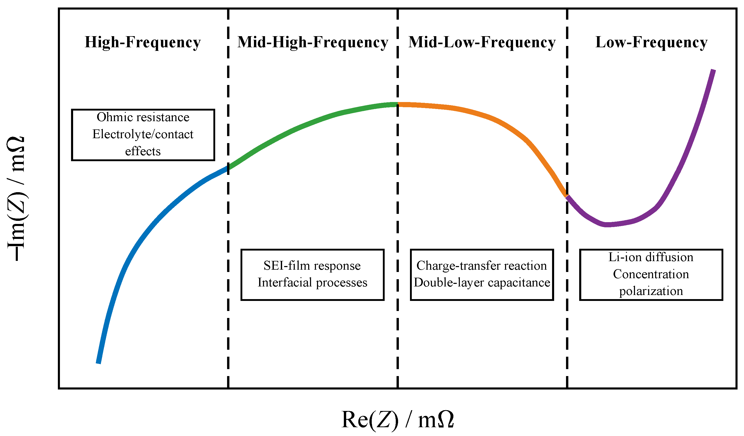
The impedance response of a lithium-ion battery varies with frequency because different internal electrochemical processes exhibit different characteristic time constants. The EIS response can be divided into four characteristic regions: high-frequency, mid-high-frequency, mid-low-frequency, and low-frequency regions. The high-frequency region is mainly associated with fast electrical responses, including ohmic contributions from the electrolyte and electrical contacts. The mid-high-frequency region is mainly influenced by interfacial-film-related processes, such as the response associated with the solid electrolyte interphase. The mid-low-frequency region primarily reflects charge-transfer kinetics and double-layer behavior at the electrode–electrolyte interface. At low frequencies, the impedance response is increasingly governed by lithium-ion diffusion and concentration polarization. It should be noted that these frequency-region boundaries are schematic rather than strictly fixed, because different electrochemical processes may overlap in the frequency domain. Therefore, EIS provides a frequency-resolved representation of the internal electrochemical state of a battery. Figure 1 schematically illustrates a typical impedance response divided into high-, mid-high-, mid-low-, and low-frequency regions.

2.2. Calculation and Representation of Complex Impedance

For a sinusoidal excitation with angular frequency ω , the complex impedance of the battery is defined in the frequency domain as
Z ( ω ) = U ( ω ) I ( ω )
where U ( ω ) and I ( ω ) denote the voltage and current responses at the corresponding frequency, respectively.
The complex impedance can be decomposed into its real and imaginary components:
Z ( ω ) = Z ( ω ) + j Z ( ω )
where Z ( ω ) denotes the real component of the impedance, Z ( ω ) denotes the imaginary component, and j = 1 .
The real and imaginary components characterize different aspects of the frequency-dependent impedance response and together preserve the information contained in the complex impedance. In a conventional Nyquist representation, the real component Z is plotted on the horizontal axis, whereas the negative imaginary component Z is plotted on the vertical axis. The evolution of the Nyquist trajectory with battery state provides an intuitive visualization of changes in the impedance response.

2.3. Principle of EIS-Based SOC Estimation

The state of charge represents the remaining available charge of a battery and is closely related to the lithiation states of the electrode materials. As SOC changes, the thermodynamic and kinetic states of the electrodes also vary. These variations can affect interfacial polarization, charge-transfer behavior, ionic transport, and diffusion processes inside the battery. Since these processes contribute to the impedance response at different characteristic frequencies, changes in SOC can be reflected in the frequency-dependent real and imaginary impedance components. The sensitivity of impedance to SOC is not uniform over the entire frequency range. Relatively slow electrochemical and transport processes contribute more strongly to the low-frequency response, whereas faster interfacial and electrical processes are represented in the medium- and high-frequency regions. Consequently, impedance features from different frequency regions may provide complementary information for SOC estimation. However, the relationship between an individual impedance component and SOC is not necessarily linear or strictly monotonic over the entire SOC range. In addition, the SOC information carried by different frequencies can overlap. Therefore, the SOC estimation problem is more appropriately regarded as a nonlinear mapping from multiple EIS features to SOC rather than as a direct one-to-one relationship between SOC and a single impedance value.
For an EIS spectrum containing N measured frequencies, the complete impedance feature vector can be expressed as
X full = [ Z ( f 1 ) , Z ( f 1 ) , Z ( f 2 ) , Z ( f 2 ) , , Z ( f N ) , Z ( f N ) ] T
Accordingly, the EIS-based SOC estimation problem can be expressed as
S O C ^ = F ( X full )
where F ( · ) represents the nonlinear mapping between the impedance features and SOC.
Although the complete EIS spectrum provides rich frequency-domain information, using all measured frequencies directly results in a relatively high-dimensional input vector. Moreover, neighboring frequencies may exhibit similar response characteristics and may therefore provide partially correlated or redundant information. Increasing the number of input frequencies consequently does not guarantee improved SOC estimation performance and may also enlarge the parameter space of the subsequent estimation model. A suitable frequency configuration should therefore retain SOC-relevant impedance information while limiting feature redundancy and unnecessary increases in input dimensionality. For a frequency configuration containing m selected frequencies, the EIS input vector is defined as
X = [ Z ( f 1 ) , Z ( f 1 ) , Z ( f 2 ) , Z ( f 2 ) , , Z ( f m ) , Z ( f m ) ] T
resulting in an input dimension of 2 m .

2.4. Overall Framework

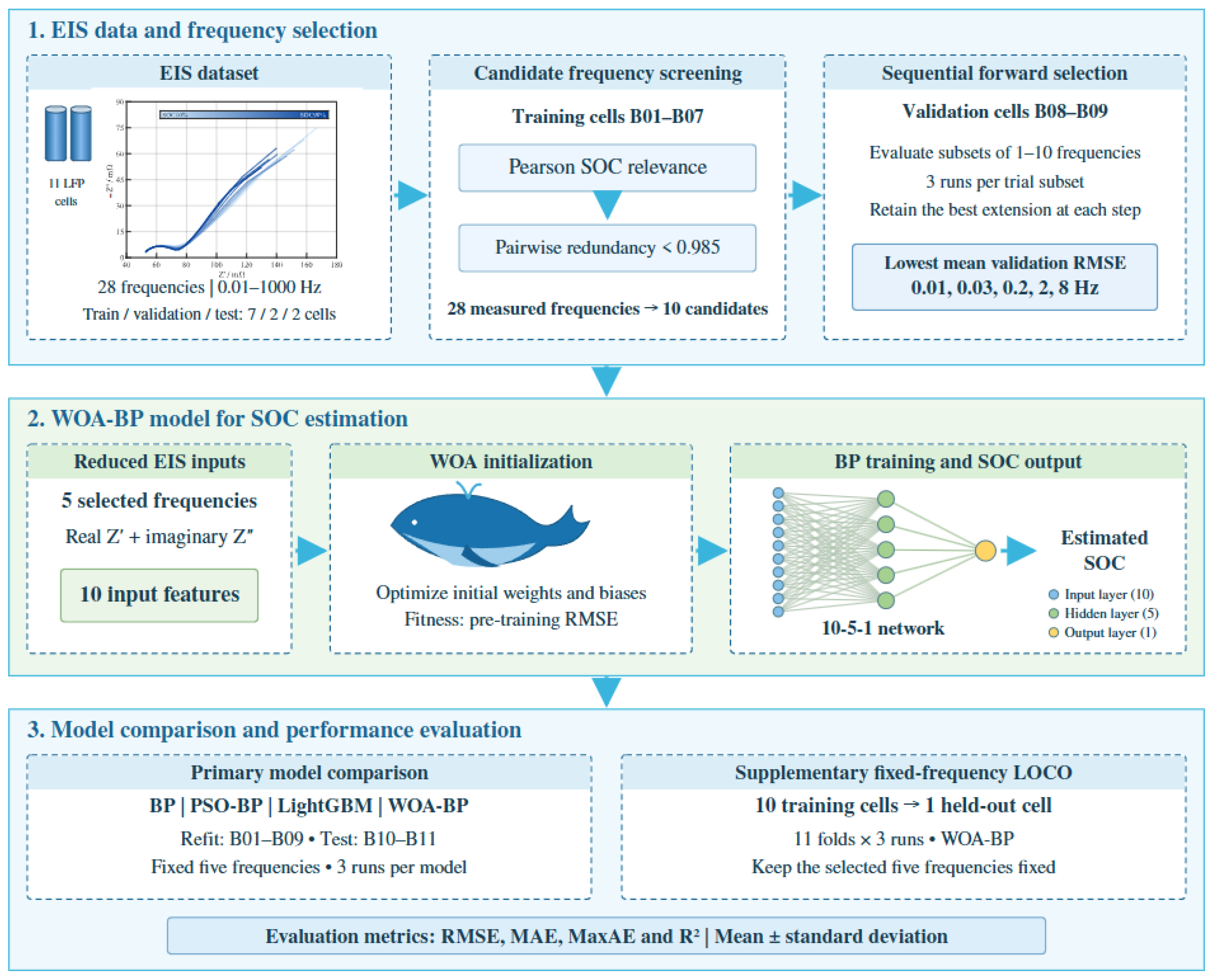
The overall framework of the proposed SOC estimation method is illustrated in Figure 2. First, the publicly available EIS–SOC dataset is preprocessed, and a fixed cell-level data partition is adopted to divide the 11 battery cells into training, validation, and test subsets. Based on the full-spectrum EIS data of the training cells, Pearson correlation analysis is employed to evaluate the association between the impedance features at different frequencies and SOC. Frequency-redundancy analysis is then further performed to preliminarily screen the original 28 frequency points and construct a candidate frequency pool. Subsequently, sequential forward selection is applied to progressively construct candidate feature subsets containing 1–10 frequency points, and the best-performing configuration along the evaluated selection path is determined according to the estimation performance on the validation cells. The five frequencies at 0.01, 0.03, 0.2, 2, and 8 Hz are selected, and the corresponding real and imaginary impedance components are extracted to construct a 10-dimensional EIS input feature vector. On this basis, the whale optimization algorithm (WOA) is employed to optimize the initial weights and biases of the backpropagation (BP) neural network, followed by local parameter refinement through BP training, thereby establishing a nonlinear WOA-BP model for SOC estimation. Finally, the proposed model is compared with conventional BP, PSO-optimized BP (PSO-BP), and Light Gradient Boosting Machine (LightGBM). With the above five frequencies fixed, an additional 11-round leave-one-cell-out evaluation is conducted, in which 10 cells are used for model training and the remaining unseen cell is used for testing in each round. This evaluation is used to systematically assess the SOC estimation performance and cross-cell generalization capability of the proposed method.

3. Dataset and Impedance Feature-Point Extraction

3.1. Public EIS–SOC Dataset

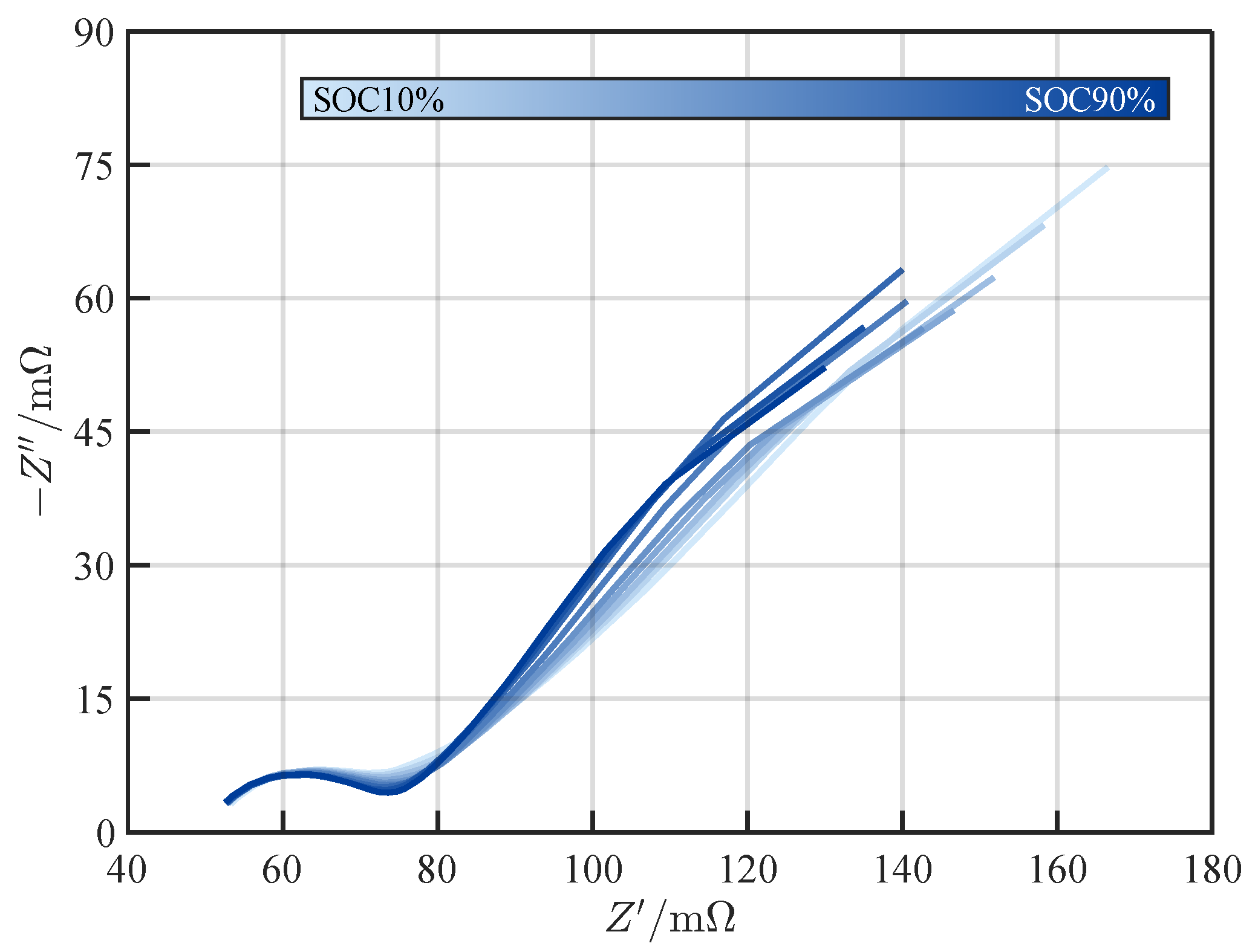
A publicly available EIS–SOC dataset of lithium-ion batteries was employed to evaluate the proposed SOC estimation method [31]. The dataset contains 11 newly manufactured cylindrical lithium iron phosphate (LFP) cells, denoted as B01–B11. Each cell has a rated voltage of 3.2 V and a rated capacity of 600 mAh. Electrochemical impedance spectroscopy measurements were performed over a wide frequency range from approximately 0.01 to 1000 Hz, providing 28 discrete frequency points for each impedance spectrum. In this study, the EIS measurements corresponding to SOC levels from 10% to 90% with an interval of 10% were used. Each EIS spectrum contains the excitation frequency together with the corresponding real and imaginary impedance components, denoted by Z and Z , respectively. These two components constitute the basic frequency-domain variables used for subsequent feature construction and SOC estimation. The main characteristics of the dataset used in this study are summarized in Table 1. To provide an intuitive overview of the SOC-dependent impedance characteristics, Figure 3 presents the mean Nyquist responses of the training cells at different SOC levels.

3.2. Data Preparation and Dataset Partition

The EIS records were organized according to cell identity, discharge-test number, and SOC level. In the primary experiment, the data were partitioned by cell identity to evaluate estimation performance on cells excluded from model development. Specifically, cells B01–B07 were assigned to the training set, B08–B09 to the validation set, and B10–B11 to the test set:
D train = { B 01 , B 02 , , B 07 }
D val = { B 08 , B 09 }
D test = { B 10 , B 11 }
The training cells were used for correlation and redundancy analysis and for fitting the models associated with candidate frequency subsets. The validation cells were used to compare these subsets and determine the frequency configuration. The test cells were excluded from frequency selection and model development. After the frequency configuration and modeling settings were determined, the training and validation cells were combined to form a final training set containing 162 samples from B01–B09. The WOA-BP models were then trained using this set and evaluated on the 36 samples from B10–B11. Each model was trained and evaluated three times while keeping the cell partition and selected frequencies fixed. Predetermined random seeds were used to control stochastic training, and the evaluation metrics were summarized as the mean and standard deviation across the three runs.
Before neural-network training, min–max normalization was applied to reduce differences in the numerical scales of the impedance features:
x ˜ = x x min x max x min
where x denotes an original feature value, and x min and x max are the minimum and maximum values of that feature in the corresponding training data. During frequency selection, the normalization parameters were calculated using B01–B07 and applied unchanged to B08–B09. For final model training, these parameters were recalculated using B01–B09 and applied unchanged to B10–B11. Validation and test features were transformed using the training-derived parameters, even when their values fell outside the training range.
An additional leave-one-cell-out evaluation was performed to examine variations in WOA-BP estimation performance across cells while keeping the frequency subset selected in the primary experiment fixed. In each fold, one cell was held out for evaluation, and the remaining ten cells were used for model training, providing 180 training samples and 18 held-out samples. Each of the 11 cells was held out once, and three training runs with different random seeds were performed per fold, resulting in 33 model fits. The normalization parameters were recalculated using only the ten training cells in each fold and then applied to the held-out cell.

3.3. Frequency Screening Based on SOC Relevance and Redundancy

The association between impedance features and SOC varies with frequency, while different frequencies may exhibit similar impedance variations. Therefore, SOC relevance and frequency redundancy were jointly considered to construct a candidate frequency pool for subsequent validation-based feature-point selection.
The analysis used only the training cells B01–B07. Repeated spectra were first aligned to a common frequency grid derived from the training data through linear interpolation in the logarithmic frequency domain. The real and imaginary impedance components from the two measurements at each cell–SOC combination were then averaged separately. This procedure produced 63 grouped observations from seven cells and nine SOC levels. These grouped observations were used for correlation and redundancy calculations, while all 126 training spectra were retained as individual samples for model fitting.
For two variables x and y, Pearson’s correlation coefficient is defined as:
r ( x , y ) = n = 1 N g ( x n x ¯ ) ( y n y ¯ ) n = 1 N g ( x n x ¯ ) 2 n = 1 N g ( y n y ¯ ) 2
where N g = 63 is the number of grouped observations, and x ¯ and y ¯ are the corresponding means. The sign of the coefficient indicates the direction of the linear association, while its absolute value describes the association strength. At each measured frequency f k , the correlations between SOC and the two impedance components were calculated as:
r Z ( f k ) = r S O C , Z ( f k ) r Z ( f k ) = r S O C , Z ( f k )
A frequency-level SOC relevance score was then defined by averaging the absolute values of these two coefficients:
S ( f k ) = r Z ( f k ) + r Z ( f k ) 2
where S ( f k ) ranges from 0 to 1. A higher score indicates a stronger average absolute linear association between the impedance components and SOC. Absolute values were used because both positive and negative associations can provide SOC-related information. This score establishes the order in which frequencies are considered during candidate screening. To assess similarity between frequencies, the redundancy score for frequencies f i and f j was defined as
ρ ( f i , f j ) = r Z ( f i ) , Z ( f j ) + r Z ( f i ) , Z ( f j ) 2
This score measures the average absolute linear correlation between the corresponding real and imaginary components at the two frequencies. Values closer to 1 indicate more similar linear variations across the grouped observations. The measured frequencies were processed in descending order of S ( f k ) . The highest-ranked frequency was retained first. Each subsequent frequency was compared with all frequencies already retained in the candidate pool. Denoting the current pool by C , a frequency f i was added when
max f j C ρ ( f i , f j ) < τ
where τ is the redundancy threshold. Otherwise, the frequency was excluded because its redundancy score with at least one retained frequency reached or exceeded the threshold. This procedure prioritizes frequencies with higher SOC relevance when highly correlated frequency pairs are encountered. In this experiment, a redundancy threshold of τ = 0.985 yielded a pool of ten candidate frequencies.

4. WOA-BP-Based SOC Estimation Method

4.1. WOA-BP Optimization Method

After the EIS feature configuration is determined, a BP neural network is employed to establish the nonlinear mapping between the multi-frequency impedance features and SOC. To reduce the influence of random initialization on BP training, the whale optimization algorithm (WOA) is introduced to optimize the initial weights and biases of the network. The resulting WOA-BP method combines the global search capability of WOA with the local parameter-refinement capability of BP training.

4.1.1. BP Neural Network

A three-layer feedforward BP neural network is employed for SOC estimation, consisting of an input layer, one hidden layer, and an output layer. For a frequency configuration containing m frequencies, the real and imaginary impedance components are simultaneously used, resulting in 2 m input features. The hidden layer contains five neurons, while the output layer contains one neuron corresponding to the estimated SOC.
For an input vector x , the output of the jth hidden neuron is expressed as
h j = g i = 1 2 m w j i ( 1 ) x i + b j ( 1 )
where w j i ( 1 ) and b j ( 1 ) denote the corresponding connection weight and bias, respectively, and g ( · ) is the hidden-layer activation function. The estimated SOC is subsequently obtained from
S O C ^ = j = 1 H w j ( 2 ) h j + b ( 2 )
where H denotes the number of hidden neurons, and w j ( 2 ) and b ( 2 ) denote the hidden-to-output weight and output bias, respectively. For the five-frequency configuration used in the final model, 10 impedance components are employed as inputs, resulting in a 10-5-1 network structure [34]. However, conventional BP uses randomly initialized weights and biases, which can lead to different initial errors and optimization trajectories. Therefore, WOA is introduced to improve the initialization of the BP network.

4.1.2. WOA-BP Optimization

WOA is a population-based metaheuristic optimization algorithm that balances global exploration and local exploitation through encircling, random search, and spiral updating mechanisms [35]. Let X ( t ) denote the position of a whale at iteration t and X * ( t ) denote the best solution obtained so far. The basic position update around the current best solution is expressed as
D = C X * ( t ) X ( t )
X ( t + 1 ) = X * ( t ) A D
A = 2 a r 1 a , C = 2 r 2
Here, r 1 and r 2 are independent random scalars uniformly sampled from [ 0 , 1 ] , and the absolute value is applied element-wise. The coefficient a decreases linearly from 2 to 0 over the iterations. For a random scalar p uniformly sampled from [ 0 , 1 ] , the encircling or random-search update is applied when p < 0.5 : the current best solution is followed when | A | < 1 , while a randomly selected whale is followed otherwise. When p 0.5 , the spiral update is applied.
To optimize BP initialization, all initial weights and biases of the network are encoded into the position vector of each whale:
θ = [ vec ( W ( 1 ) ) , b ( 1 ) , W ( 2 ) , b ( 2 ) ] T
Therefore, each whale represents one complete set of BP initial parameters rather than an individual network parameter.
For the 10-5-1 network, the parameter vector consists of 50 input-to-hidden weights, 5 hidden-layer biases, 5 hidden-to-output weights, and 1 output bias. Thus, the WOA search dimension is
D = 10 × 5 + 5 + 5 + 1 = 61
The fitness of each whale is evaluated using the training RMSE before BP local training:
Fitness ( θ ) = 1 N i = 1 N S O C i S O C ^ i ( θ ) 2
A smaller fitness value indicates a more favorable initialization of the BP network. After the WOA search is completed, the best candidate vector is decoded into the initial weights and biases of the BP network.
For comparison, conventional BP and PSO-BP are also established using the same network structure and EIS input features. The conventional BP model uses randomly initialized weights and biases, whereas PSO-BP employs particle swarm optimization to search for more favorable initial weights and biases before BP training. After the optimization process, the obtained parameters are used to initialize the BP network, followed by the same local training procedure. In addition, LightGBM is introduced as an independent non-BP machine-learning baseline using the same selected EIS features, enabling comparison with a different nonlinear modeling framework.

4.1.3. Optimization Procedure

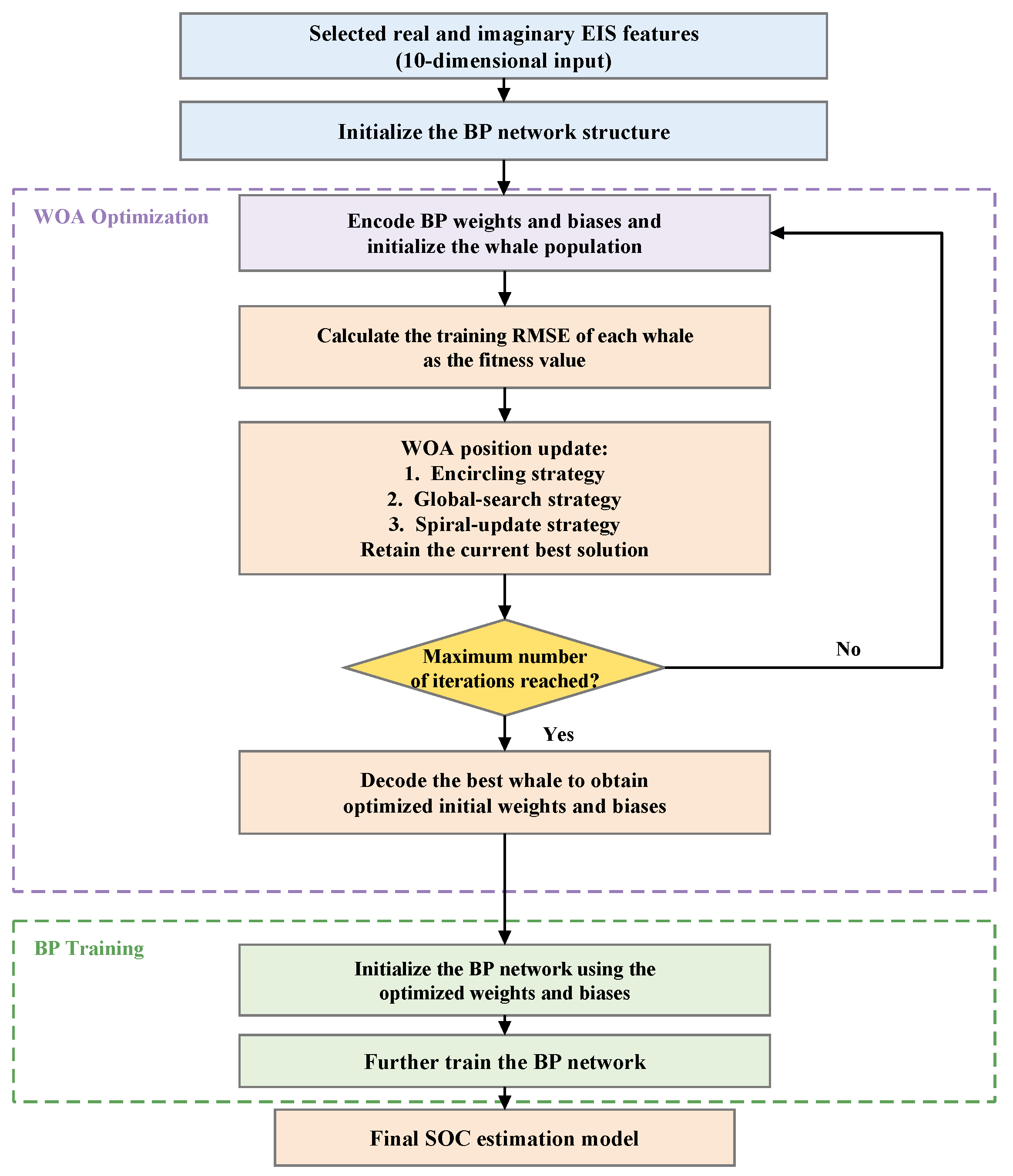
The complete WOA-BP optimization procedure is illustrated in Figure 4. First, the selected real and imaginary impedance features are used to construct the input vector, and the BP network structure is initialized. All BP weights and biases are then encoded to initialize the whale population. For each whale, the training RMSE before BP training is calculated as the fitness value. During each WOA iteration, whale positions are updated according to the encircling, global-search, or spiral-update strategy, and the best candidate solution is continuously retained. When the maximum number of iterations is reached, the best whale is decoded to obtain the optimized initial weights and biases of the BP network. These optimized parameters are then used to initialize the BP network, which is further trained to obtain the final SOC estimation model.

5. Results and Discussion

5.1. Experimental Setup and Evaluation Metrics

The BP-based models and the overall evaluation procedure were implemented in MATLAB R2024a, while LightGBM was implemented using Python 3.7.8 with the LightGBM 4.6.0 library. BP, PSO-BP, WOA-BP, and LightGBM were evaluated using the same five-frequency, 10-dimensional EIS feature representation and the same cell-level data partition. The three BP-based models employed the same network structure and local training settings. LightGBM was introduced as an additional non-BP machine-learning baseline to provide a comparison with a different nonlinear modeling framework. The SOC estimation performance was evaluated using RMSE, mean absolute error (MAE), maximum absolute error (MaxAE), and the coefficient of determination ( R 2 ), which are defined as
R M S E = 1 N i = 1 N ( S O C ^ i S O C i ) 2
M A E = 1 N i = 1 N S O C ^ i S O C i
M a x A E = max 1 i N S O C ^ i S O C i
R 2 = 1 i = 1 N ( S O C i S O C ^ i ) 2 i = 1 N ( S O C i S O C ¯ ) 2
Here, N is the number of samples, S O C i and S O C ^ i denote the reference and estimated SOC values, respectively, and S O C ¯ is the mean reference SOC. RMSE reflects the overall estimation error and is more sensitive to relatively large deviations, MAE represents the average absolute error, and MaxAE characterizes the largest individual estimation error. A higher R 2 indicates better agreement between the estimated and reference SOC values.

5.2. EIS Characteristic Analysis and Multi-Frequency Feature-Point Extraction

5.2.1. Full-Spectrum EIS Characteristics

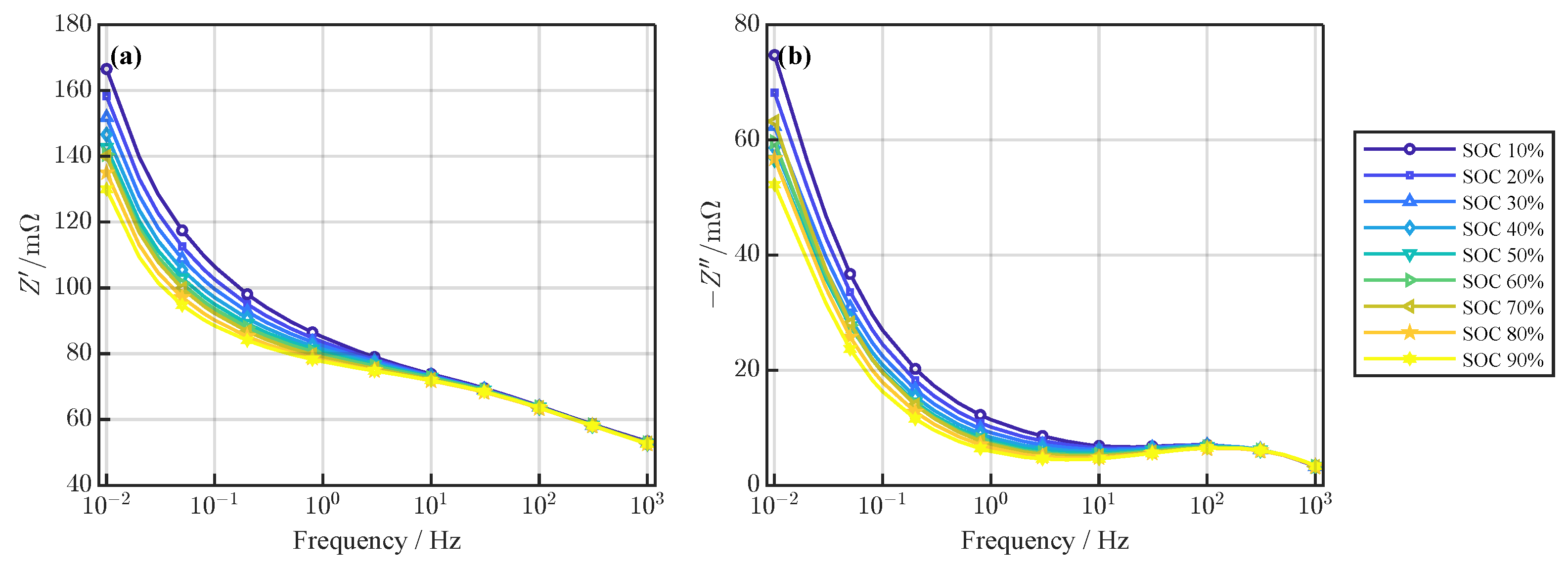
To investigate the distribution of SOC-related information over the measured EIS spectrum, the real impedance Z and negative imaginary impedance Z of the training cells were first analyzed over the complete frequency range. Figure 5 presents the mean impedance responses at different SOC levels as functions of frequency.
As shown in Figure 5a, the real impedance decreases with increasing frequency. At low frequencies, the curves corresponding to different SOC levels exhibit pronounced separation. As the frequency increases, the separation gradually narrows, and the curves become closely grouped at high frequencies. Figure 5b also shows greater separation among the negative imaginary impedance responses at low frequencies. However, their ordering with SOC is not strictly monotonic throughout this region. At higher frequencies, the differences among SOC levels become less pronounced. These observations indicate that the magnitude and pattern of SOC-related impedance variations depend on frequency and differ between the real and imaginary components. The relatively pronounced separation at low frequencies motivates further examination of these features for SOC estimation. However, the separation of mean curves alone does not establish the predictive value of individual frequencies or the additional information provided by combining them. Therefore, SOC relevance and inter-frequency redundancy are subsequently quantified to construct a candidate frequency pool, followed by validation-based evaluation of the frequency configurations.

5.2.2. SOC Relevance and Inter-Frequency Redundancy Analysis

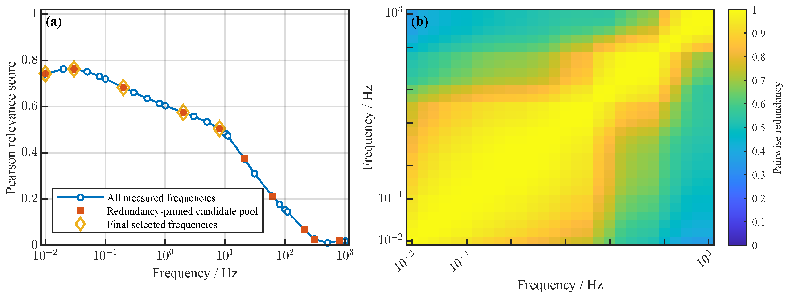
Following the screening method described in Section 3.3, the SOC relevance scores and pairwise redundancy were calculated using the training data. The pairwise redundancy analysis in Figure 6 shows substantial redundancy within several frequency regions. The score combines the absolute Pearson correlations of the real and imaginary impedance components with SOC.
Figure 6a presents the Pearson relevance scores of the measured frequencies with respect to SOC. The relevance score reaches its maximum of approximately 0.763 at 0.03 Hz and generally decreases toward higher frequencies. For example, the scores at 0.2, 2, and 8 Hz are approximately 0.683, 0.575, and 0.505, respectively. This pattern indicates stronger overall linear associations with SOC in the lower-frequency region of the present training dataset. Figure 6b shows substantial pairwise redundancy within several frequency regions. For example, although 0.02 and 0.05 Hz have high SOC relevance scores, their redundancy with 0.03 Hz reaches approximately 0.9976 and 0.9972, respectively. Both frequencies are therefore removed after 0.03 Hz is retained, using the redundancy threshold of 0.985. In contrast, the redundancy between 0.01 and 0.03 Hz is approximately 0.9802, allowing 0.01 Hz to remain in the candidate pool. These examples illustrate how relevance ranking and redundancy screening jointly determine candidate retention. The screening procedure reduces the 28 measured frequencies to ten candidates: 0.01, 0.03, 0.2, 2, 8, 21, 61, 210, 310, and 810 Hz. This threshold-based screening removes highly redundant frequencies but does not make the retained features mutually uncorrelated. In addition, no minimum SOC relevance threshold is imposed, so some higher-frequency candidates with low relevance scores remain available for subsequent evaluation. Their contribution to SOC estimation is assessed through the validation-based sequential forward-selection procedure, rather than inferred from correlation scores alone.

5.2.3. Validation of Frequency Configurations

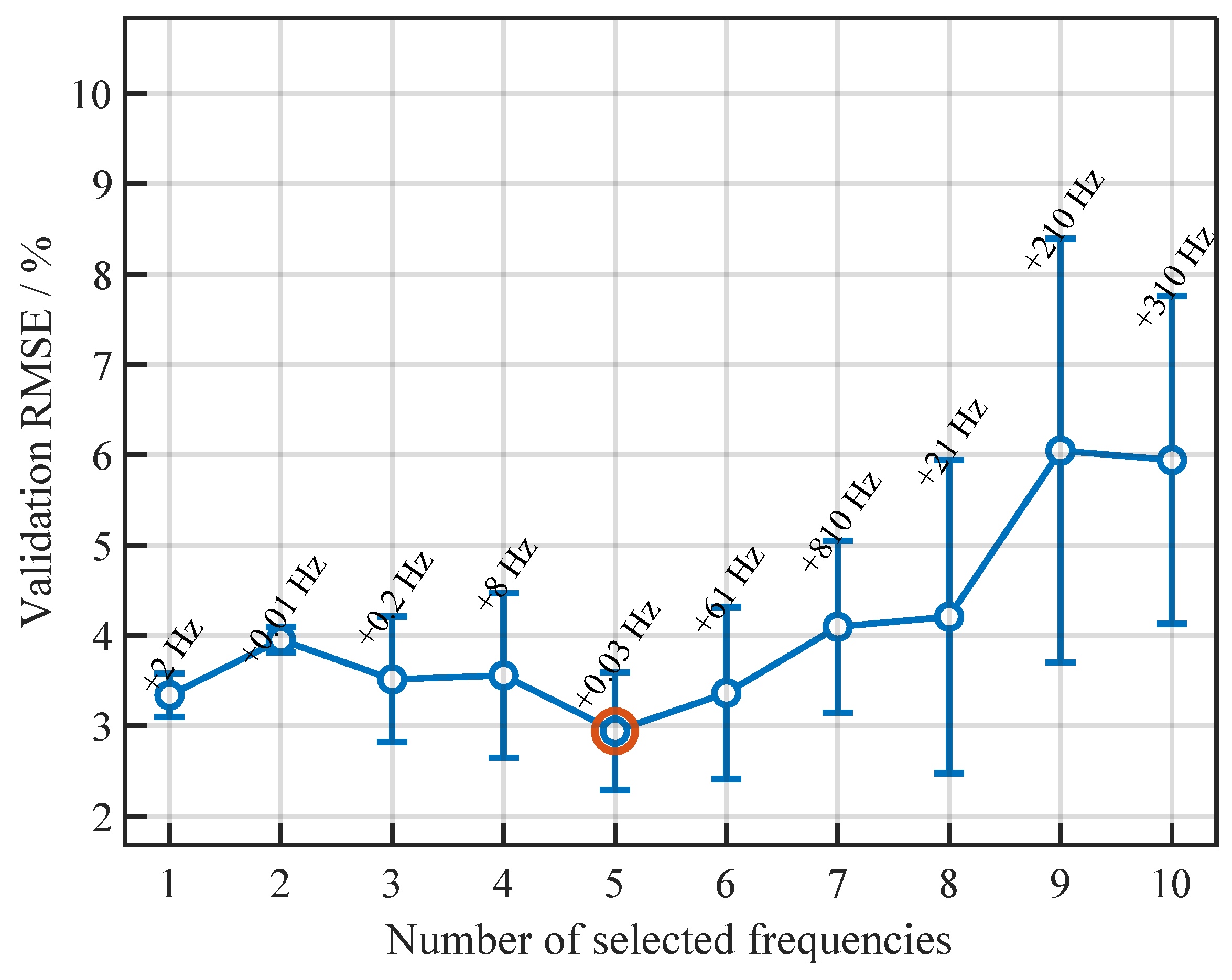
Starting from the ten candidates obtained through redundancy screening, sequential forward selection was performed using the fixed training and validation cells. First, each candidate frequency was individually evaluated using WOA-BP. The frequency yielding the lowest mean validation RMSE over three runs was selected as the starting point. Subsequently, each remaining candidate was separately added to the current configuration, and the combination with the lowest mean validation RMSE was retained at each step. The same three random seeds were used for competing configurations within each step. This procedure continued until all ten candidates were included. The test cells did not participate in frequency selection. Table 2 presents the resulting selection path and validation RMSE.
Figure 7 illustrates the variation in validation RMSE along the selection path. The error does not decrease monotonically as frequencies are added. The single-frequency configuration at 2 Hz achieves a mean RMSE of 3.34%, whereas adding 0.01 Hz increases it to 3.95%. With subsequent additions, the five-frequency configuration achieves the lowest mean validation RMSE of 2.94 ± 0.65 %. Further increasing the number of frequencies does not improve this result, and the ten-frequency configuration yields an RMSE of 5.94 ± 1.81 %.
These results indicate that increasing the number of impedance frequencies does not necessarily improve SOC estimation under the present data split and model settings. Based on the lowest mean validation RMSE along the evaluated path, the frequencies at 0.01, 0.03, 0.2, 2, and 8 Hz were selected for subsequent model comparisons. Their real and imaginary impedance components form a 10-dimensional input vector, representing an approximately 82.1% reduction relative to the 56 components of the complete measured spectrum.

5.3. Contribution of WOA to BP Optimization

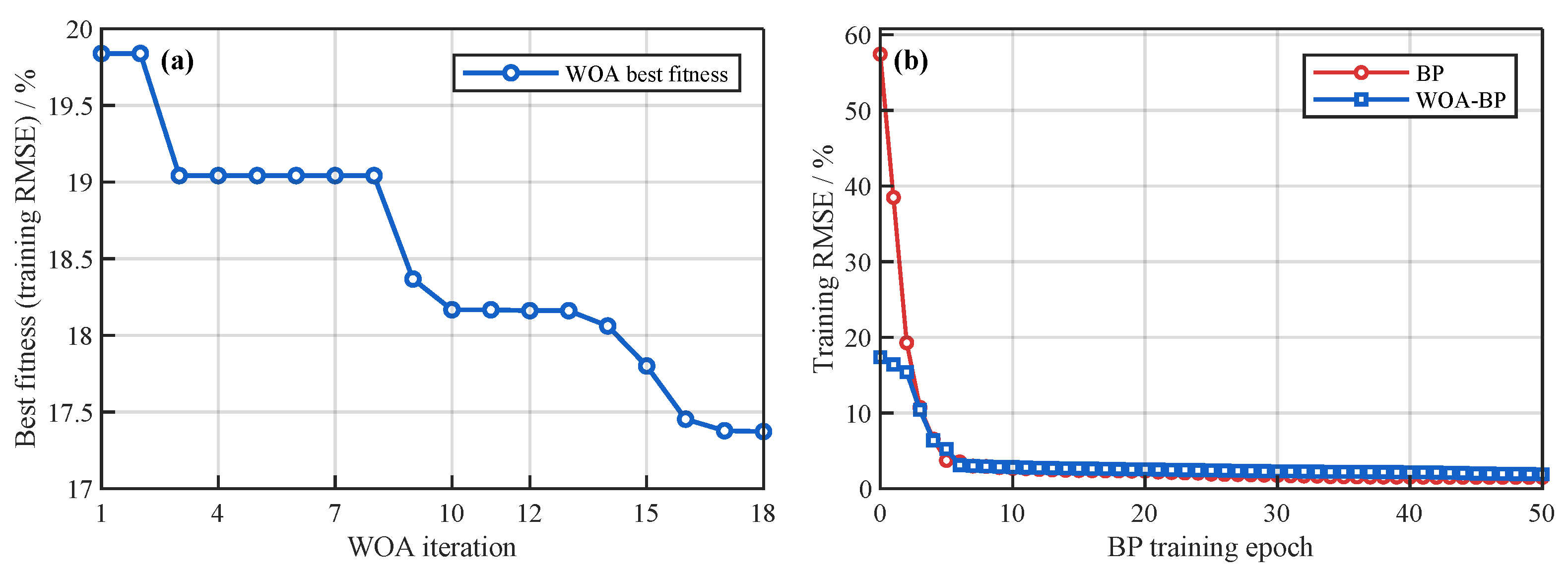
To further investigate the contribution of WOA to the proposed model, Figure 8 illustrates the WOA optimization process and the subsequent BP training behavior representative predefined run. As shown in Figure 8a, the best fitness decreases from approximately 19.84% to 19.04% during the early iterations and then progressively decreases to approximately 17.37%. Since the training RMSE before BP local training is used as the WOA fitness function, the decreasing fitness indicates that WOA progressively identifies initial weights and biases with lower prediction errors.
Figure 8b further compares the early training RMSE of conventional BP and WOA-BP. The randomly initialized BP network starts with an RMSE of approximately 57.42%, whereas the WOA-initialized network starts at approximately 17.37%, indicating that the best solution found by WOA provides a more favorable starting point for BP training. As training proceeds, the RMSE of both models decreases rapidly and the difference between the two curves gradually becomes smaller. WOA therefore first searches globally for a favorable initial region in the parameter space, after which BP further refines the network parameters through local optimization. In this way, WOA-BP combines global initialization search with local gradient-based optimization for SOC estimation.

5.4. Comparative SOC Estimation Results and Discussion

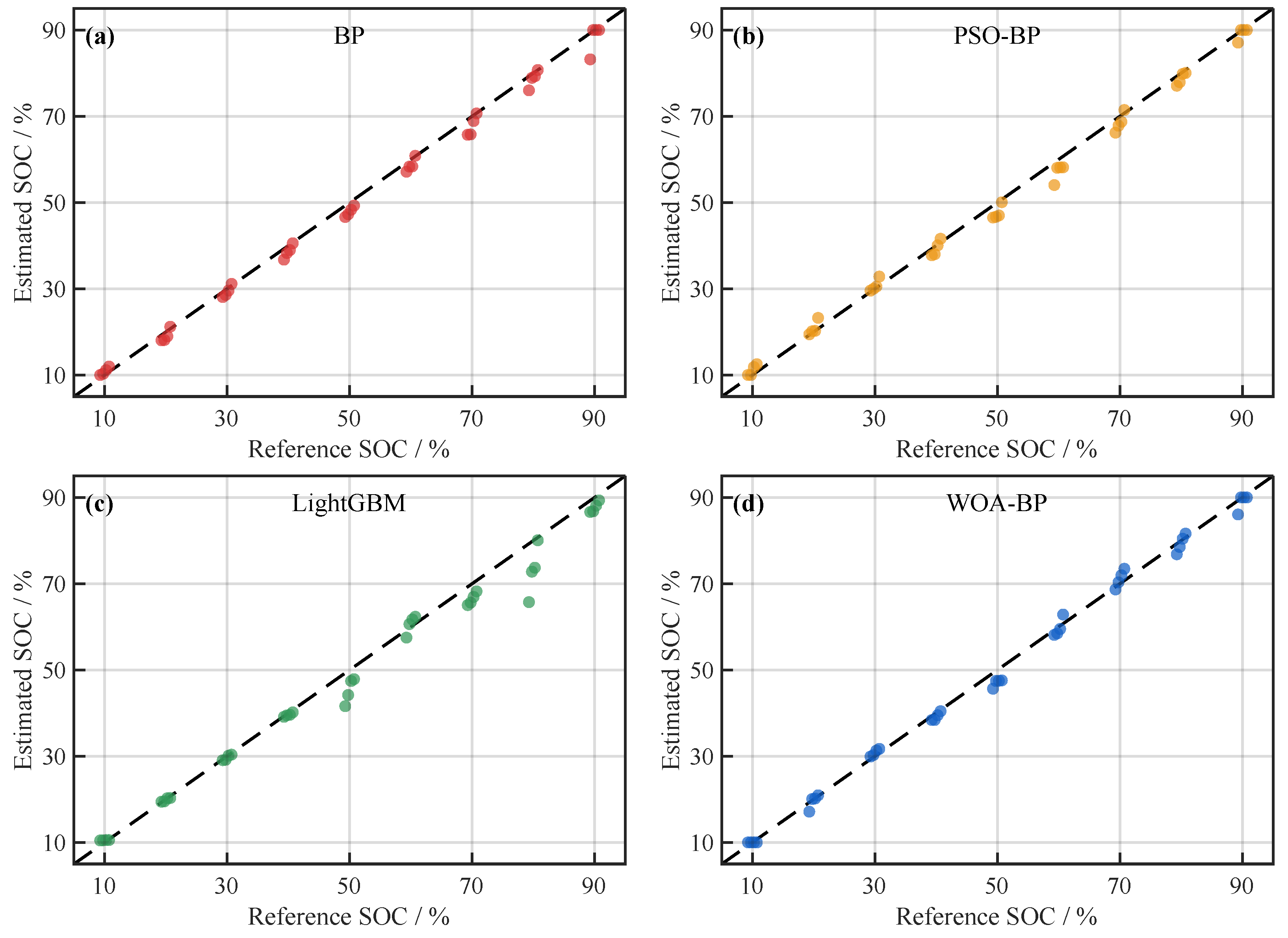
The SOC estimation performance of BP, PSO-BP, LightGBM, and WOA-BP was further evaluated on the independent test cells using the same five-frequency inputs. Figure 9 compares the estimated SOC values with the reference SOC values for a representative predefined run, where the dashed line represents ideal estimation. The BP model generally follows the reference SOC, although noticeable deviations remain at several SOC levels. PSO-BP also achieves close agreement with the reference values but exhibits deviations for some samples in the intermediate SOC range. LightGBM provides relatively accurate predictions for many samples but shows larger deviations at some SOC levels, particularly at 80% SOC. In comparison, the WOA-BP predictions are generally distributed close to the ideal reference line over the investigated SOC range.
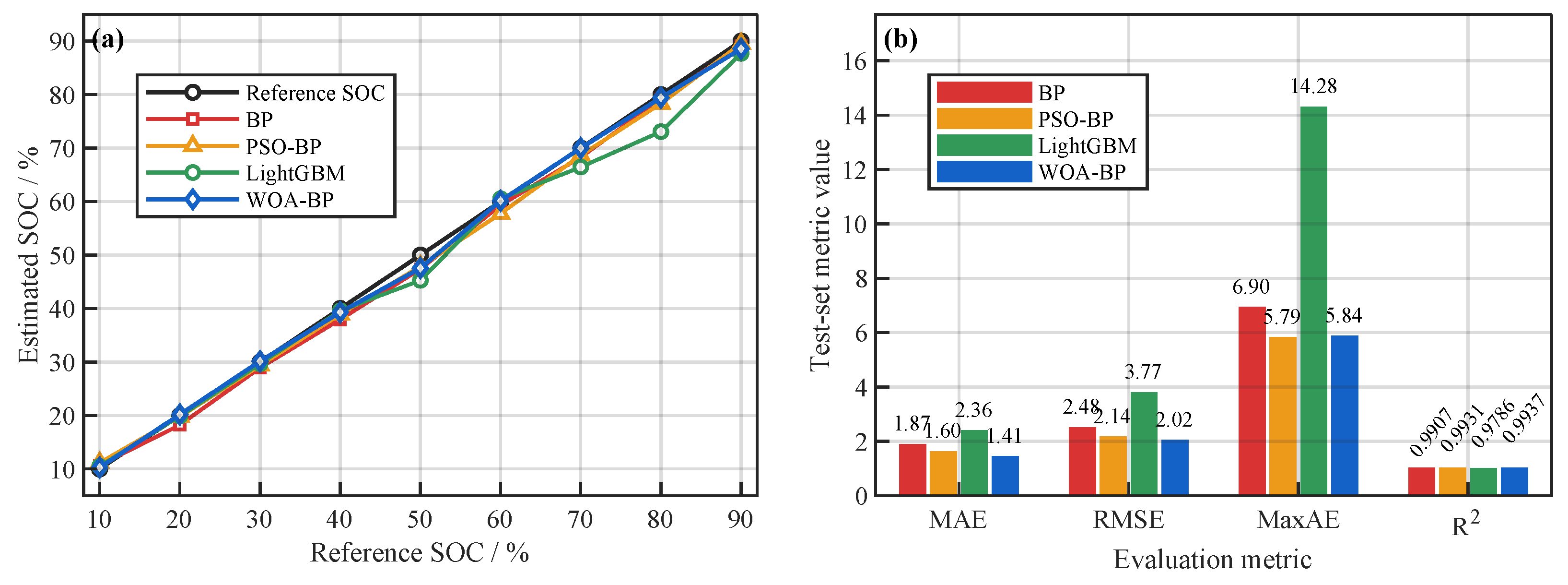
Figure 10a further compares the SOC prediction trends of the four models. The predicted SOC values at each reference SOC level were averaged over the three independent runs. Figure 10b presents the corresponding mean MAE, RMSE, MaxAE, and R 2 values over the same three runs. Table 3 further reports the mean values and standard deviations for all four models.
Across the three runs, BP achieves a mean RMSE of 2.48%, a mean MAE of 1.87%, a mean MaxAE of 6.90%, and a mean R 2 of 0.9907. PSO-BP improves the overall performance relative to BP, yielding a mean RMSE of 2.14%, a mean MAE of 1.60%, and the lowest mean MaxAE of 5.79%. LightGBM yields a mean RMSE of 3.77%, a mean MAE of 2.36%, and a mean MaxAE of 14.28%, indicating larger individual deviations for some samples. The proposed WOA-BP achieves the lowest mean RMSE of 2.02%, the lowest mean MAE of 1.41%, and the highest mean R 2 of 0.9937, while its mean MaxAE is 5.84%. Its mean RMSE is reduced by approximately 18.84%, 5.58%, and 46.57% compared with BP, PSO-BP, and LightGBM, respectively.

5.5. Leave-One-Cell-Out Evaluation with Fixed Frequencies

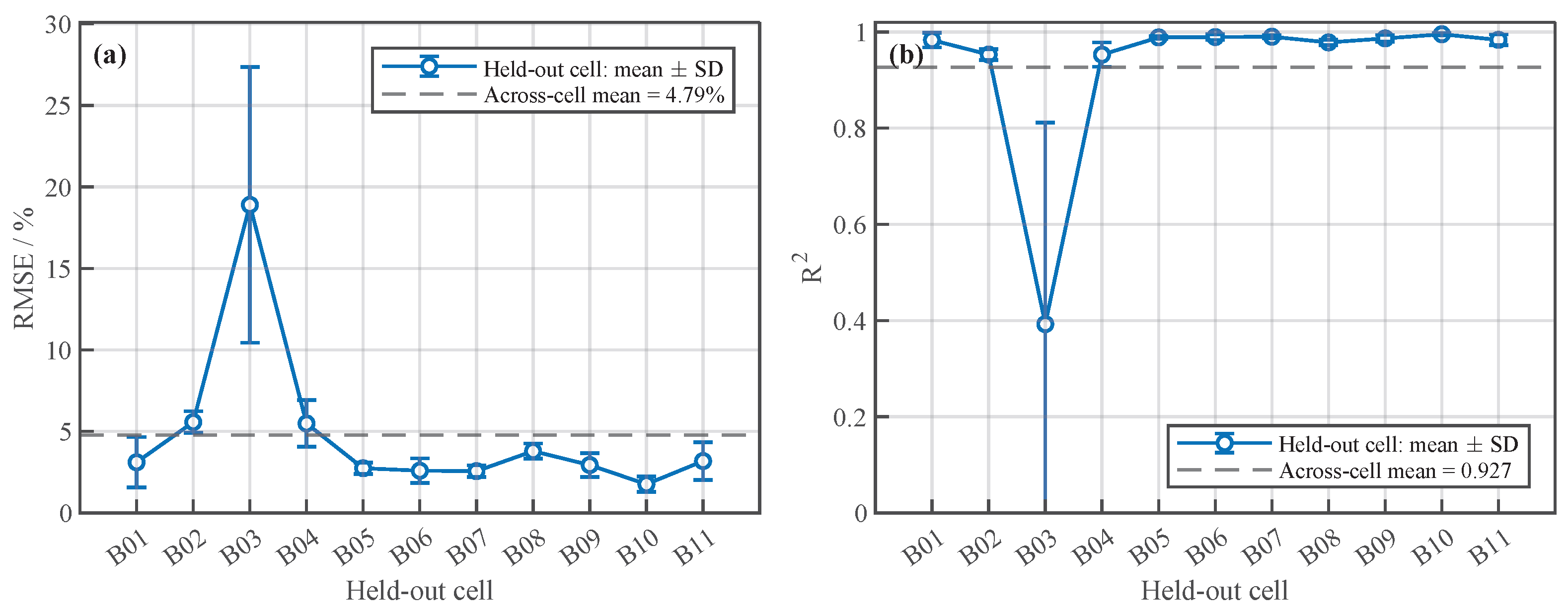
To examine the performance of the selected frequency configuration across different cells, a supplementary leave-one-cell-out (LOCO) evaluation was conducted [33]. The five frequencies at 0.01, 0.03, 0.2, 2, and 8 Hz were kept fixed throughout this evaluation. In each fold, one cell was held out for testing, while the remaining ten cells were used to train WOA-BP. Input normalization was fitted using only the training cells in each fold. Three runs were performed per fold, resulting in 33 model fits across the eleven cells. Figure 11 presents the mean RMSE and R 2 for each held-out cell, with error bars indicating the standard deviations over three runs. Eight of the eleven cells achieve a mean RMSE below 5%. B10 yields the lowest mean RMSE of 1.76 ± 0.47 %, whereas B02 and B04 yield 5.57 ± 0.66 % and 5.49 ± 1.44 %, respectively. B03 exhibits a substantially higher mean RMSE of 18.90 ± 8.46 % and a lower mean R 2 of 0.3925 ± 0.4192 , indicating both larger estimation errors and greater variation across runs.
Averaging the eleven cell-wise mean RMSE values gives an across-cell mean of 4.79%, while their median is 3.11%. The corresponding across-cell mean R 2 is 0.9266. The difference between the mean and median RMSE reflects the influence of the large errors for B03. Thus, although the fixed-frequency model provides relatively low errors for most cells, its performance varies considerably with the held-out cell. The favorable results on the predefined test split therefore do not imply uniformly accurate estimation across all cells.

6. Conclusions

This study developed a data-driven SOC estimation method based on multi-frequency impedance feature-point extraction and a WOA-BP neural network. Using data from eleven lithium iron phosphate cells, Pearson relevance analysis and redundancy screening reduced the 28 measured frequencies to ten candidates. Validation-based sequential forward selection then identified a five-frequency configuration comprising 0.01, 0.03, 0.2, 2, and 8 Hz. The corresponding real and imaginary impedance components formed a 10-dimensional input vector, reducing the input dimensionality by approximately 82.1% relative to the complete spectrum. This configuration achieved the lowest mean validation RMSE along the evaluated selection path, demonstrating that increasing the number of frequency points does not necessarily improve estimation performance.
WOA optimized the initial weights and biases of the BP network, followed by local parameter refinement through BP training. On the predefined test cells, the resulting WOA-BP model achieved a mean RMSE of 2.02%, a mean MAE of 1.41%, a mean MaxAE of 5.84%, and a mean R 2 of 0.9937 over three runs. Its mean RMSE was approximately 18.84%, 5.58%, and 46.57% lower than those of BP, PSO-BP, and LightGBM, respectively, under the same selected frequency configuration. WOA-BP achieved the lowest mean RMSE and MAE, whereas PSO-BP exhibited a slightly lower mean MaxAE and smaller variation across runs. The supplementary fixed-frequency leave-one-cell-out evaluation revealed variation in estimation performance across cells. Eight of the eleven cells achieved a mean RMSE below 5%, while B03 exhibited substantially larger errors. The across-cell mean and median RMSE were 4.79% and 3.11%, respectively. These results indicate that the favorable performance on the predefined test split does not imply uniformly accurate estimation across cells.
The present findings are limited to the investigated dataset and SOC range. Moreover, the reduction in input dimensionality does not establish a proportional reduction in measurement time, particularly because the selected configuration retains 0.01 Hz. Future work will extend the evaluation to more diverse cells, temperatures, and aging states, jointly consider estimation accuracy and acquisition time in frequency selection, and independently validate the complete selection and modeling pipeline.

Author Contributions

Conceptualization, Y.W. (Yi Wang) and C.F.; methodology, Y.W. (Yi Wang); validation, Y.W. (Yi Wang), Y.W. (Yuxuan Wen) and Y.L.; formal analysis, Y.W. (Yi Wang); data curation, Y.W. (Yi Wang); writing—original draft preparation, Y.W. (Yi Wang); writing—review and editing, Y.W. (Yi Wang) and C.F.; visualization, Y.W. (Yi Wang); supervision, C.F.; funding acquisition, C.F. All authors have read and agreed to the published version of the manuscript.

Funding

The project was supported by Natural Science Foundation of the Jiangsu Higher Education Institutions of China Grant 25KJB470014 and the Postgraduate Research & Practice Innovation Program of Jiangsu Province Grant 26CXJH4336.

Data Availability Statement

The data presented in this study are available on request from the corresponding author.

Conflicts of Interest

The authors declare no conflict of interest.

Abbreviations

The following abbreviations are used in this manuscript:
LIBsLithium-ion batteries
SOCState of charge
BMSBattery management system
OCVOpen-circuit voltage
ECMEquivalent circuit model
EISElectrochemical impedance spectroscopy
LFPLithium iron phosphate
BPBackpropagation
PSOParticle swarm optimization
WOAWhale optimization algorithm
PSO-BPParticle swarm optimization-optimized BP
WOA-BPWhale optimization algorithm-optimized BP
RMSERoot mean square error
MAEMean absolute error
MaxAEMaximum absolute error

References

  1. Peng, J.; Qian, X.; Xu, X.; Wu, W.; Wang, J.; Wang, R.; Yang, H.Y.; Ye, J.; Wu, Y. State of Charge Estimation Techniques for Lithium-Ion Batteries: A Review. Energy Technol. 2025, 13, 2500542. [Google Scholar] [CrossRef] [Scilit]
  2. Jiang, M.; Li, D.; Li, Z.; Chen, Z.; Yan, Q.; Lin, F.; Yu, C.; Jiang, B.; Wei, X.; Yan, W.; et al. Advances in battery state estimation of battery management system in electric vehicles. J. Power Sources 2024, 612, 234781. [Google Scholar] [CrossRef] [Scilit]
  3. Hussein, H.M.; Aghmadi, A.; Abdelrahman, M.S.; Rafin, S.S.H.; Mohammed, O. A review of battery state of charge estimation and management systems: Models and future prospective. Wiley Interdiscip. Rev. Energy Environ. 2024, 13, e507. [Google Scholar]
  4. Zhang, J.; Che, Y.; Teodorescu, R.; Song, Z.; Hu, X. Energy storage management in electric vehicles. Nat. Rev. Clean Technol. 2025, 1, 161–175. [Google Scholar] [CrossRef] [Scilit]
  5. Chaudhari, T.; Chakravorty, S. Analysis and advancements of the state of charge estimation methods in smart battery management system supported by lithium-ion battery operated electric vehicles. Next Energy 2025, 8, 100337. [Google Scholar] [CrossRef] [Scilit]
  6. Pisani Orta, M.A.; García Elvira, D.; Valderrama Blaví, H. Review of state-of-charge estimation methods for electric vehicle applications. World Electr. Veh. J. 2025, 16, 87. [Google Scholar] [CrossRef] [Scilit]
  7. Zhao, F.; Guo, Y.; Chen, B. A review of lithium-ion battery state of charge estimation methods based on machine learning. World Electr. Veh. J. 2024, 15, 131. [Google Scholar] [CrossRef] [Scilit]
  8. Takyi-Aninakwa, P.; Wang, S.; Liu, G.; Bage, A.N.; Masahudu, F.; Guerrero, J.M. An enhanced lithium-ion battery state-of-charge estimation method using long short-term memory with an adaptive state update filter incorporating battery parameters. Eng. Appl. Artif. Intell. 2024, 132, 107946. [Google Scholar] [CrossRef] [Scilit]
  9. Du, J.; Wang, J.; Tan, B.; Cao, X.; Qu, C.; Ou, Y.; He, X.; Xiong, L.; Tu, R. Estimation of battery state of charge based on changing window adaptive extended Kalman filtering. J. Energy Storage 2024, 103, 114325. [Google Scholar] [CrossRef] [Scilit]
  10. Fan, C.; Liu, K.; Ren, Y.; Peng, Q. Characterization and identification towards dynamic-based electrical modeling of lithium-ion batteries. J. Energy Chem. 2024, 92, 738–758. [Google Scholar] [CrossRef] [Scilit]
  11. Tao, Z.; Zhao, Z.; Wang, C.; Huang, L.; Jie, H.; Li, H.; Hao, Q.; Zhou, Y.; See, K.Y. State of charge estimation of lithium batteries: Review for equivalent circuit model methods. Measurement 2024, 236, 115148. [Google Scholar] [CrossRef] [Scilit]
  12. Wang, C.; Yang, M.; Wang, X.; Xiong, Z.; Qian, F.; Deng, C.; Yu, C.; Zhang, Z.; Guo, X. A review of battery SOC estimation based on equivalent circuit models. J. Energy Storage 2025, 110, 115346. [Google Scholar] [CrossRef] [Scilit]
  13. Tian, J.; Chen, C.; Shen, W.; Sun, F.; Xiong, R. Deep learning framework for lithium-ion battery state of charge estimation: Recent advances and future perspectives. Energy Storage Mater. 2023, 61, 102883. [Google Scholar] [CrossRef] [Scilit]
  14. Sun, Q.; Yu, X.; Li, H.; Fan, J. Adaptive feature extraction and fault diagnosis for three-phase inverter based on hybrid-CNN models under variable operating conditions. Complex Intell. Syst. 2022, 8, 29–42. [Google Scholar] [CrossRef] [Scilit]
  15. Xu, L.; Wen, Z.; Su, H.; Cola, S.; Fabbian, N.; Feng, Y.; Yang, S. An innovative method integrating two deep learning networks and hyperparameter optimization for identifying fiber optic temperature measurements in earth-rock dams. Adv. Eng. Softw. 2025, 199, 103802. [Google Scholar] [CrossRef] [Scilit]
  16. Wu, Y.; Bai, D.; Zhang, K.; Li, Y.; Yang, F. Advancements in the estimation of the state of charge of lithium-ion battery: A comprehensive review of traditional and deep learning approaches. J. Mater. Inform. 2025, 5, 18. [Google Scholar] [CrossRef] [Scilit]
  17. Sun, Q.; Yu, X.; Li, H.; Peng, F.; Sun, G. Fault detection for power electronic converters based on continuous wavelet transform and convolution neural network. J. Intell. Fuzzy Syst. 2022, 42, 3537–3549. [Google Scholar] [CrossRef] [Scilit]
  18. Sun, Q.; Yang, L.; Li, H.; Sun, G. RUL prediction for AECs of power electronic systems based on machine learning and error compensation. J. Intell. Fuzzy Syst. 2023, 44, 7407–7417. [Google Scholar] [CrossRef] [Scilit]
  19. Zhang, C.; Xu, X.; Li, Y.; Huang, J.; Li, C.; Sun, W. Research on SOC estimation method for lithium-ion batteries based on neural network. World Electr. Veh. J. 2023, 14, 275. [Google Scholar] [CrossRef] [Scilit]
  20. Hai, N.; Wang, S.; Liu, D.; Gao, H.; Fernandez, C. An improved random drift particle swarm optimization-feed forward backpropagation neural network for high-precision state-of-charge estimation of lithium-ion batteries. J. Energy Storage 2023, 73, 109286. [Google Scholar] [CrossRef] [Scilit]
  21. Yao, J.; Kowal, J. Towards a smarter battery management system: A critical review on deep learning-based state of charge estimation of lithium-ion batteries. Energy AI 2025, 21, 100585. [Google Scholar] [CrossRef] [Scilit]
  22. Hou, J.; Xu, J.; Lin, C.; Jiang, D.; Mei, X. State of charge estimation for lithium-ion batteries based on battery model and data-driven fusion method. Energy 2024, 290, 130056. [Google Scholar] [CrossRef] [Scilit]
  23. Fan, C.; Liu, Y.; Liu, K.; Li, M.; Turgun, Y.; Peng, Q. Two-stage prediction–correction with residual compensation: A framework for robust state of charge estimation under cross-temperature conditions. J. Energy Storage 2026, 175, 123275. [Google Scholar] [CrossRef] [Scilit]
  24. Xu, M.; Zhang, E.; Wang, S.; Shen, Y.; Zou, B.; Li, H.; Wan, Y.; Wang, K.; Jiang, K. Dynamic ultrasonic response modeling and accurate state of charge estimation for lithium ion batteries under various load profiles and temperatures. Appl. Energy 2024, 355, 122210. [Google Scholar] [CrossRef] [Scilit]
  25. Fan, Y.; Yan, C.; Wu, X.; Li, Y.; Dou, W.; Gao, G.; Zhang, P.; Guan, Q.; Tan, X. Mechanical stress-based state-of-charge estimation for lithium-ion batteries via deep learning techniques. Energy 2025, 326, 136216. [Google Scholar] [CrossRef] [Scilit]
  26. Liu, J.; Shi, J.; Hao, F.; Dai, M. A novel enhanced global exploration whale optimization algorithm based on Lévy flights and judgment mechanism for global continuous optimization problems. Eng. Comput. 2023, 39, 2433–2461. [Google Scholar] [CrossRef] [Scilit]
  27. Wei, M.; Ye, M.; Zhang, C.; Lian, G.; Xia, B.; Wang, Q. Robust state of charge estimation of LiFePO4 batteries based on Sage_Husa adaptive Kalman filter and dynamic neural network. Electrochim. Acta 2024, 477, 143778. [Google Scholar] [CrossRef] [Scilit]
  28. Nováková, K.; Papež, V.; Sadil, J.; Knap, V. Review of electrochemical impedance spectroscopy methods for lithium-ion battery diagnostics and their limitations. Monatshefte Chem.-Chem. Mon. 2024, 155, 227–232. [Google Scholar] [CrossRef] [Scilit]
  29. Guo, J.; Xu, Y.; Li, P.; Pedersen, K.; Gaberšček, M.; Stroe, D.I. Can electrochemical impedance spectroscopy be replaced by direct current techniques in battery diagnosis? ChemPhysChem 2024, 25, e202400528. [Google Scholar] [CrossRef] [Scilit]
  30. Santoni, F.; De Angelis, A.; Moschitta, A.; Carbone, P.; Galeotti, M.; Cinà, L.; Giammanco, C.; Di Carlo, A. A guide to equivalent circuit fitting for impedance analysis and battery state estimation. J. Energy Storage 2024, 82, 110389. [Google Scholar] [CrossRef] [Scilit]
  31. Mustafa, H.; Bourelly, C.; Vitelli, M.; Milano, F.; Molinara, M.; Ferrigno, L. SOC estimation on Li-ion batteries: A new EIS-based dataset for data-driven applications. Data Brief 2024, 57, 110947. [Google Scholar] [CrossRef] [Scilit]
  32. Fan, C.; Zhang, K.; Peng, Q.; Tian, J.; Liu, K.; Chung, C.Y. Fast characterization of lithium-ion battery impedance and nonlinearity using optimized multisine perturbation signal. IEEE Trans. Ind. Electron. 2025, 72, 11395–11405. [Google Scholar] [CrossRef] [Scilit]
  33. Yuan, Y.; Jiang, B.; Chen, Q.; Wang, X.; Wei, X.; Dai, H. A comparative study of battery state-of-charge estimation using electrochemical impedance spectroscopy by different machine learning methods. Energy 2025, 328, 136658. [Google Scholar] [CrossRef] [Scilit]
  34. Ströbel, M.; Pross-Brakhage, J.; Kopp, M.; Birke, K.P. Impedance based temperature estimation of lithium ion cells using artificial neural networks. Batteries 2021, 7, 85. [Google Scholar] [CrossRef] [Scilit]
  35. Mirjalili, S.; Lewis, A. The Whale Optimization Algorithm. Adv. Eng. Softw. 2016, 95, 51–67. [Google Scholar] [CrossRef] [Scilit]
Figure 1. Schematic illustration of a typical EIS response divided into different frequency regions.
Batteries 12 00378 g001
Figure 2. Overall framework of the proposed multi-frequency impedance feature-point extraction-based SOC estimation method.
Batteries 12 00378 g002
Figure 3. Mean Nyquist responses of the training cells at different SOC levels.
Batteries 12 00378 g003
Figure 4. Flowchart of the WOA-BP optimization procedure for SOC estimation.
Batteries 12 00378 g004
Figure 5. Full-spectrum impedance characteristics at different SOC levels: (a) real impedance Z and (b) negative imaginary impedance Z .
Batteries 12 00378 g005
Figure 6. Frequency relevance and inter-frequency redundancy analysis: (a) SOC relevance scores of the measured frequencies; (b) pairwise inter-frequency redundancy between the measured frequencies.
Batteries 12 00378 g006
Figure 7. Validation RMSE along the sequential forward-selection path. Error bars indicate standard deviations over three runs. The orange circle highlights the selected five-frequency configuration with the lowest mean validation RMSE along the evaluated path.
Batteries 12 00378 g007
Figure 8. WOA-BP optimization and training convergence: (a) WOA best-fitness convergence and (b) training RMSE of BP and WOA-BP.
Batteries 12 00378 g008
Figure 9. SOC prediction scatter plots on the independent test cells for a representative predefined run: (a) BP, (b) PSO-BP, (c) LightGBM, and (d) WOA-BP. The dashed line represents the ideal estimation.
Batteries 12 00378 g009
Figure 10. Comparative SOC estimation performance averaged over three independent runs: (a) mean predicted SOC at each reference SOC level and (b) mean MAE, RMSE, MaxAE, and R 2 of the four models.
Batteries 12 00378 g010
Figure 11. Fixed-frequency LOCO performance of WOA-BP: (a) RMSE; (b) R 2 . Error bars indicate standard deviations over three runs per cell, and dashed lines indicate across-cell means.
Batteries 12 00378 g011
Table 1. Main characteristics of the public EIS–SOC dataset used in this study.
ParameterValue
Battery chemistryLithium iron phosphate (LFP)
Cell typeCylindrical
Number of cells11 (B01–B11)
Rated voltage3.2 V
Rated capacity600 mAh
Number of discharge testsTwo per cell
EIS frequency range0.01–1000 Hz
Number of measured frequencies28
SOC range used in this study10–90%
SOC interval10%
Table 2. Sequential frequency selection and validation. RMSE (mean ± standard deviation over three runs).
Number of
Frequencies
Added
Frequency (Hz)
Frequency Configuration (Hz)Validation
RMSE (%)
122 3.34 ± 0.24
20.010.01, 2 3.95 ± 0.14
30.20.01, 0.2, 2 3.51 ± 0.69
480.01, 0.2, 2, 8 3.56 ± 0.91
50.030.01, 0.03, 0.2, 2, 8 2.94 ± 0.65
6610.01, 0.03, 0.2, 2, 8, 61 3.36 ± 0.95
78100.01, 0.03, 0.2, 2, 8, 61, 810 4.10 ± 0.95
8210.01, 0.03, 0.2, 2, 8, 21, 61, 810 4.21 ± 1.73
92100.01, 0.03, 0.2, 2, 8, 21, 61, 210, 810 6.05 ± 2.35
103100.01, 0.03, 0.2, 2, 8, 21, 61, 210, 310, 810 5.94 ± 1.81
Note: Bold indicates the frequency configuration with the lowest mean validation RMSE along the evaluated sequential forward-selection path.
Table 3. SOC estimation performance on the independent test cells (mean ± standard deviation over three runs).
ModelRMSE (%)MAE (%)MaxAE (%) R 2
BP 2.48 ± 0.26 1.87 ± 0.18 6.90 ± 0.83 0.9907 ± 0.0019
PSO-BP 2.14 ± 0.19 1.60 ± 0.11 5.79 ± 0.21 0.9931 ± 0.0012
LightGBM 3.77 ± 0.00 2.36 ± 0.00 14.28 ± 0.00 0.9786 ± 0.0000
WOA-BP 2.02 ± 0.39 1.41 ± 0.30 5.84 ± 1.35 0.9937 ± 0.0025
Note: Bold indicates the best mean performance for each metric among the compared models: the lowest RMSE, MAE, and MaxAE, and the highest R 2 .
Disclaimer/Publisher’s Note: The statements, opinions and data contained in all publications are solely those of the individual author(s) and contributor(s) and not of MDPI and/or the editor(s). MDPI and/or the editor(s) disclaim responsibility for any injury to people or property resulting from any ideas, methods, instructions or products referred to in the content.