Data-Driven Modeling of Auxiliary Consumption in Utility-Scale BESS

Abstract

Accurately modeling the auxiliary power consumption of Battery Energy Storage Systems (BESSs) is increasingly important as grid-scale storage assets are becoming involved in electricity markets. In this paper, we develop a data-driven framework to characterize and forecast auxiliary consumption using operational data from a utility-scale BESS deployed in Italy. To capture the short-term thermal inertia of the system and the delayed response of the cooling systems, a set of predictors based on moving averages of power and ambient temperature is constructed. Two novel modeling approaches are proposed: a three-dimensional look-up table (LUT) representation that provides an interpretable characterization of system behavior, as well as a Random Forest (RF) regression model capable of capturing complex non-linear relationships between parameters. These are evaluated in comparison with a two-dimensional LUT from the literature. The analysis showed a superior performance of the RF model that comes at the cost of reduced interpretability and computational efficiency, while both proposed models outperform the literature-based LUT. Moreover, the impact of the number and type of predictors on model performance is systematically assessed, to shed light on what constitutes the requirements for a reasonably accurate estimation of the auxiliary systems. Finally, the concept of forecasting uncertainty for the temperature and day-ahead forecasting applicability for the auxiliary systems is investigated by introducing a persistence-based logic and an evaluation of the impact on the results. Overall, the study highlights the importance of explicitly modeling auxiliary consumption in grid-scale BESSs, proposes well-performing models for its estimation, and provides practical guidelines for their implementation in energy management and forecasting applications.

1. Introduction

Global efforts to decarbonize the energy system focus on a drastic reduction in greenhouse emissions to meet the Paris Agreement targets and limit global warming. The ambitious decarbonization targets include achieving net-zero emissions by 2050 and significantly scaling up clean energy deployment by 2030 to electrify emerging rural areas and to support the electrification of loads, such as the cases of electric vehicles and heat pumps. These strategies are outlined by the International Energy Agency’s (IEA) Net Zero Roadmap and COP28 energy goals, which aim to triple the renewable energy capacity and double energy efficiency during this decade. However, due to their inherent intermittency and partial predictability, they pose two key challenges to the traditional power system paradigm: first, the temporal mismatch between consumption and generation complicates real-time energy balancing; and, second, the variability in generation can cause voltage and frequency regulation issues, stressing the grid stability [1]. Thus, integrating high shares of variable renewables into the electric grid requires significant upgrades in transmission infrastructure, flexibility mechanisms, and energy storage solutions in order to maintain reliability and stability. For example, authors in the USA [2] investigated various scenarios coupling demand, generation, and weather trends, simulated on synthetic grid topologies, and concluded that, regardless of the scenario, the net demand curves get deeper in the middle of the day, leading to extremely volatile electricity prices and outages leading to the loss of load events.

This need, paramount to the safe and reliable operation of the future power system [3], has given a meteoric rise in the procurement of Battery Energy Storage Systems (BESSs), most notably, the larger installations connected directly to the electrical transmission or distribution network, known as grid-scale BESSs. Their attractiveness comes from the wide range of services that they can provide to support the energy transition and the integration of RES, often more quickly and efficiently than their traditional counterparts. In their special Batteries and Secure Energy Transitions report [4] published in 2024, the IEA states that the global BESS installments rose from approximately 1 GW in 2013, to 85 GW in 2023, 42 GW of which were added in that year alone, showing a strong recent trend. However, specific deployment patterns differ across regions. For example, Europe has seen a strong inclination towards behind-the-meter installations driven by high retail prices, whereas grid-scale installations have remained economically infeasible.

The need for more strategically planned grid-scale installations has been widely recognized by national regulators and public bodies in Europe, leading to the integration of BESS capacity market frameworks and similar long-term procurement mechanisms. For example, Italy has introduced a dedicated support mechanism for utility-scale electricity storage established under Legislative Decree No. 210/2021. Thus, the first official auction took place at the end of 2025, awarding incentives to 10 GWh of grid-scale BESSs to enter service by 2028. Similarly, Poland’s capacity market has allocated 2.5 GW for delivery by 2029, with similar mechanisms being activated across the continent to support long-term system adequacy. These measures support large-scale deployment, ensure system adequacy, and maintain economic feasibility by reducing the financial uncertainty caused by both the rapid changes in the power systems, as well as the evolving cost trends of the technology itself. Indeed, looking at the future outlook, the IEA Net Zero Emissions (NZE) scenario forecasts BESS installations to rise to an astounding 1200 GW, 1000 GW of which would be grid-scale [4].

The anticipated expansion of grid-scale storage introduces unique complexities that extend beyond the scope of the vast amount of conventional battery research focusing on the cell technology. These complexities arise from the sheer size and multitude of the components, dynamic operation conditions, and interaction with electricity markets, requiring specific tools to optimize their operational and economic performance over the assets’ lifetime. Until recently, the limited deployment of utility-scale BESSs, coupled with the high costs associated with detailed system-level studies, has constrained the research in this area. A wide overview of the modeling approaches for grid-connected storage technologies was recently published in [5], where the authors indeed note “generic modeling” as one of their conclusions and defended that, even though it comes with certain benefits, its drawback is the lack of case- and technology-specific details which can lead to reduced accuracy.

The authors in [6] noted this gap and focused on bridging the existing modeling methods for Li-Ion cells to stationary grid-scale BESSs by building a Thevenin equivalent circuit populated by Open-Circuit Voltage (OCV) and internal resistance measurements. However, the focus is still solely on the battery pack and does not completely bridge the gap; instead, it aims to represent the BESS as one large cell and avoid the need for single-cell testing. Similar effort was done by the work presented in [7] that utilized an equivalent circuit model to model the State-of-Charge (SoC) of a BESS for off-grid applications. In general, grid-scale BESSs are modeled with a fixed efficiency that aims to represent all the losses that occur during the charging and discharging processes [8]. However, this over-generalization fails to grasp specific non-linear dependencies that are difficult to characterize, such as those arising in cooling systems, as well as well-defined non-linear loss mechanisms like ohmic losses in wires and transformers.

An analytical approach was proposed in [9], where the authors developed separate models for efficiency and auxiliary consumption. The auxiliary demand is estimated through a thermal model based on Joule losses, combined with an HVAC coefficient of performance to represent the cooling power required to remove heat. While this is a well-structured analytical representation, it treats the BESS as a closed system driven mainly by internally generated heat, without explicitly accounting for external influences such as ambient temperature or site-specific conditions. This represents a significant simplification with respect to real utility-scale operation. The authors in [10] laid the groundwork for a more detailed, data-driven modeling of a large-scale BESS specifically for power grid applications, where the model included not only the battery pack, but also the Power Conversion System (PCS) and auxiliaries. The paper proposes a test procedure to develop a look-up table (LUT)-based model for characterizing BESS performance. This includes efficiency and power-delivery capability as a function of SoC and power, as well as the auxiliary power consumption as a function of ambient temperature and power. The end goal was a more accurate estimation of the potential to provide services, to assure compliance with the capacity offered on the market. The model developed was subsequently applied to evaluate the overall BESS efficiency during ancillary service provision [11], simulating several operating profiles and seasonal conditions. The authors compared the simulations, including auxiliary consumption, against a base case in which they were neglected. The analysis showed that the impact was more significant for low-power operation and longer idle periods, especially in the summer period when, due to external heat, the thermal-management demand persists independently of the BESS operation. In this scenario, the study reported significant errors of up to 10% in the estimated operational efficiency [11]. The results showed that this effect depends on the BESS’s utilization, highlighting the importance of accounting for auxiliary consumption with dedicated modeling—especially when the asset is underutilized. The work in [12] goes one step beyond and proposes SoC restoration techniques utilizing the participation to the Ancillary Services Market (ASM), where the authors found that the SoC restoration requirements are 25–45% of the energy dedicated to service provision themselves, severely impacting the technical and economical dispatch of the asset.

The overview of grid-scale-focused BESS models showed that auxiliary power consumption is often overlooked, typically incorporated together with the battery pack in a simplified manner, rather than treated as a separate component. In other cases such as the model proposed in [10], the authors correctly point out its importance, but with a simplification that does not account for the preceding thermal or operational history, such as moving averages (MAs) and cumulative effects. Aside from the energy exchanged with the grid, a BESS continuously absorbs energy to support equipment such as thermal management systems, control hardware, and safety apparatus. In particular, cooling units required to maintain battery cells within safe operating temperatures could account for a meaningful share of the overall energy throughput, especially under variable ambient conditions and dynamic operating modes. Failing to properly account for this additional consumption can lead to inaccurate SoC estimates, which, in turn, could cause infeasible dispatch schedules, reduced reserve availability for the power system, and financial losses for the asset owner.

The main contribution of the paper is to provide a methodology for accurately estimating and forecasting the auxiliary consumption of grid-scale BESSs, going beyond a simple function of instantaneous parameters, which is the current best practice. The proposed approach is validated through a real-life case study, demonstrating its applicability to an asset actively providing grid services. By explicitly forecasting auxiliary consumption, the proposed framework enables more reliable SoC estimation, and an improved assessment of both technical and economic performance.

The remaining part of the paper is organized as follows: Section 2 presents the concept of an auxiliary consumption and outlines possible techniques to forecast it. Section 3 describes a case study and the modeling framework to model and forecast the auxiliary consumption in a utility-scale BESS, whereas Section 4 presents the simulation results and analyzes key observations in parameter selection. Finally, Section 5 provides a comprehensive discussion, concludes the paper, and provides future research directions.

2. Auxiliary Consumption in Battery Energy Storage Systems

In a broad sense, auxiliary load in a BESS refers to the electric power consumed by supporting subsystems that are necessary for the operation, safety, control, and protection of a BESS, but do not contribute to storing or delivering energy to the grid. This includes the thermal management systems, and the monitoring systems alongside the sensors, as well as any additional equipment including but not limited to transformers, switchboards, and instrumentation power. In modern BESSs, by far the largest contributor is the thermal management system. However, in real-life deployments, auxiliary consumption is typically available only as an aggregate measurement, whereas a quantitative breakdown among each component is unavailable. Moreover, component-level consumption and internal control logics are often proprietary and not disclosed to the asset manager. Therefore, a general system-level modeling perspective is a reasonable tradeoff that accurately addresses these data availability constraints.

Temperature is widely recognized as a dominant factor influencing lithium-ion batteries’ performance, degradation, and safety. Operating at low temperatures leads to an increased internal resistance and reduced power capability, whereas elevated temperatures accelerate ageing mechanisms, affecting the system reliability and lifetime [13,14]. These effects are particularly critical because during normal operation at ambient conditions, lithium-ion batteries generally generate heat due to charge transfer processes and electrochemical reactions. Heat generation strongly depends on operating conditions such as the current rate (C-rate), SoC, and internal resistance, and may become significant during high-power operation [15]. Nevertheless, it should be noted that the tests were performed on a relatively small battery with a very high C-rate. Consequently, the battery temperature results from the combined effect of internally generated heat and external environmental conditions, making thermal control a fundamental requirement rather than an optional design feature. For these reasons, an effective Battery Thermal Management System (BTMS) is essential in order to maintain batteries within their optimal temperature range and ensure a consistent performance over a wide range of operating conditions and overtime [14,16]. The thermal management of lithium-ion batteries has been widely investigated in the literature, leading to a variety of works discussing the trade-offs between different strategies. In that sense, several review articles provide comprehensive classifications of BTMS distinguishing between air-based, liquid-based, and advanced or hybrid solutions [16,17]. Although the details of these systems are outside of scope of this paper, the literature agrees that no single strategy outperforms the rest across all operating conditions. More importantly, recent overviews emphasize that thermal management should be analyzed at the system level considering the operation dynamics and external conditions [18].

In practical modeling terms, these systems do not behave as constant or proportional loads that can be easily represented by offsets. On the contrary, their power consumption is strongly dependent on both the temperature dynamics and control behavior, leading to a non-linear, state-dependent behavior that can affect overall performance over its lifetime. Although direct experimental evidence for large-scale BESSs is scarce, extensive studies in the Electric Vehicle (EV) and Heating, Ventilation, and Air Conditioning (HVAC) domains demonstrate that auxiliary energy consumption exhibits a strong non-linear dependence on ambient temperature [19,20]. On top of this, the literature has demonstrated that machine-learning algorithms can be an effective pathway towards modeling auxiliary consumption, with [19] proposing the XGBoost model to predict auxiliary consumption in an EV and enhance the energy management system. Auxiliary demand increases sharply outside moderate temperature ranges, with distinct regimes associated with heating and cooling operation. These behaviors depend not only on the thermal load intensity, but also on control logic and compressor cycling, leading to discontinuous and history-dependent power consumption. Thermal inertia further amplifies non-linear behavior. The large thermal mass of battery assemblies causes delayed temperature responses, leading to prolonged cooling or heating cycles even after operating conditions change. As a result, the auxiliary power demand depends not only on the instantaneous temperature, but may also be impacted by the recent thermal history of the system [21]. This effect is particularly relevant for containerized BESSs, where thermal equilibrium is rarely instantaneous.

3. Materials and Methods

This chapter presents the modeling framework proposed to reconstruct and forecast the auxiliary consumption of a utility-scale BESS. The analysis is focused on real-life operational data, and focuses on understanding how ambient temperature and battery utilization influence the thermal inertia of the system and, thus, its thermal management demand. It should be noted that the thermal inertia of a utility-scale BESS could not be accurately represented by a single characteristic time constant, as the response of the HVAC system depends not only on passive thermal dynamics, but also on control settings, power perturbations, and ambient temperature transients, as well as previous state of the container. Therefore, we treat the thermal inertia as an aggregate, adopting a data-driven approach that aims to arrive at a “characteristic-time-constant-like” evaluation, without imposing a rigid physical thermal model.

After introducing the technical characteristics of the case study and describing the preprocessing steps, an exploratory analysis is conducted to identify the main drivers of auxiliary consumption and to investigate the role of thermal inertia. In addition, the analysis of the auxiliary consumption shows that it represents a non-negligible share of the total delivered energy, emphasizing the need for accurate forecasting. Building on these insights, two parallel modeling approaches are proposed, and compared against a literature-based model.

First, a two-dimensional LUT-based model was proposed in [10], serving as a reference found in the state-of-the-art model. Second, a non-parametric three-dimensional LUT is constructed using a stochastic discretization procedure. Last, a Random Forest (RF) model is implemented to overcome the dimensionality limitations of the LUT and to better capture non-linear interactions between the target parameters. Within this approach, a structured predictor-expansion framework is proposed to systematically evaluate the contribution of moving-average predictors and to compare the performance of the approaches proposed.

3.1. Case Study Description

The BESS considered in this study is located in Sardinia, Italy, and entered operation in July 2023. The plant was contracted within the pilot project promoted by Terna for the provision of the Fast Reserve service, aimed at improving the dynamic frequency response of the power system during the first instants following frequency disturbances. Outside these availability windows, as well as for the remaining uncontracted capacity, the BESS can participate in the energy market, enabling additional revenue streams and operational flexibility.

The BESS is a Lithium Iron Phosphate (LFP) electrochemical storage system with a rated power of 14.7 MW and an energy capacity of 8.8 MWh. The plant is characterized by a modular and hierarchical architecture: it is divided into four nominally identical feeders, connected in parallel at the high-voltage node. Each feeder is interfaced through a double secondary transformer, featuring two low-voltage secondary windings on the battery side. Each secondary winding supplies two power conversion systems (inverters), which are, in turn, connected to an aggregated control unit of the storage system, referred to as the Battery Administration Unit (BAU). Each BAU supervises and controls three Battery Cluster Units (BCUs) connected in parallel. Overall, the plant includes 16 BAUs and 48 BCUs. At the lowest level of the hierarchy, each BCU comprises 15 battery modules connected in series, with each module consisting of 24 individual cells.

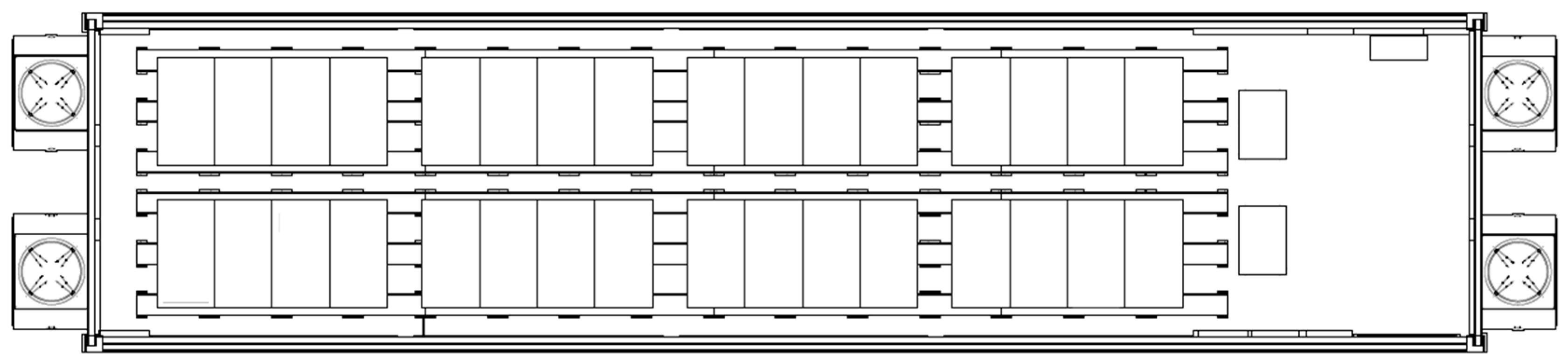
Given the geographical location of the site, the thermal management of the BESS relies exclusively on an air-based cooling system, implemented through industrial HVAC units installed within the battery containers. No active heating system or heat pump is present. The thermal dynamics of the system are therefore predominantly associated with heat removal from the battery containers, driven by internal heat generation during charge and discharge operations and by external ambient conditions. The auxiliary system’s aim is thus to maintain the internal temperature of the battery enclosures within a target range of approximately 23–28 °C. This temperature window represents a compromise between enabling high C-rate operation—required for fast frequency response services—and limiting battery degradation, thereby preserving long-term system performance and reliability. The cooling system is structured by separating the BCUs into different containers. Each container contains sixteen BCUs and is equipped with four HVAC units as shown in Figure 1. A separate fifth feeder is provided to supply all the auxiliaries in the system, comprising the HVAC units from the three containers.

3.2. Data Description and Preprocessing

The data collection from the physical plant spanned between the months of September 2023 and November 2024, allowing for 13 months of samples. The main variables of interest were the power exchanged by the BESS (P_BESS), the ambient temperature measured by the nearby weather station (T_amb), and the consumption of the auxiliaries that are fed by a separate feeder (P_aux). Furthermore, an additional set of temperature measurements for each cluster unit (T_clus,i) was analyzed exclusively for exploratory purposes, aiming to understand the containers’ thermal behavior and the system’s thermal management. Instead, they were not utilized for the modeling itself and fall outside of the main parameters for the approaches that are proposed. The measurements were obtained through individual measurement devices and sampled with a 5-min resolution. 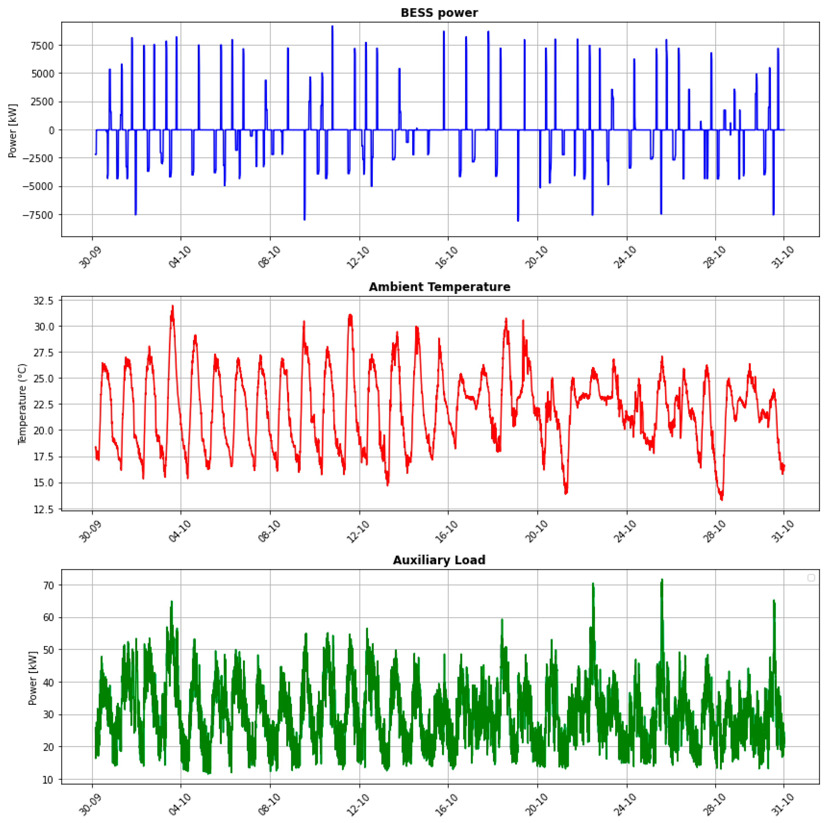Figure 2 depicts a sample time series used in the analysis, showing the main input variables for the period of October 2023, where the BESS power is expressed according to the generator sign convention. Even over this short window, the auxiliary consumption never really drops to zero, and, through the idle stretches, it appears to follow the ambient temperature more closely than the BESS operation.

The first step was to resample the dataset to a 15-min interval, following the time discretization of the Italian Electricity Market, excluding timestamps in which at least one of the parameters contained corrupted data. Corrupted data was identified as either missing or unphysical values far outside of nominal values, attributed to measurement or communication errors. In practice, this issue occurred only in the power measurements and was limited to less than 0.5% of the samples, most of which were simply missing. Further filtering was not applied to avoid misrepresentation of normal behavior as irregular. In practice, anything below a 15-min time interval would not provide a meaningful benefit. Moreover, all models rely on the absolute value of the BESS output, as heat generation is mainly related to the magnitude of the power, rather than its direction. As previously introduced, the main idea is to gain understanding of how the power output of the BESS and the ambient temperature affect the consumption of the auxiliary systems; then, this knowledge can serve to build a forecasting service.

3.3. Exploratory Data Analysis

In order to gain understanding about the dataset and make initial hypotheses correlated to the findings in the literature, an exploratory campaign was initiated. The initial question was to better understand the utilization of the BESS and to form assumptions on the impact of its scheduling and operation on the consumption of the auxiliaries. First, an analysis of the daily auxiliary consumption was conducted by comparing the daily auxiliary energy with the total daily energy exchanged by the BESS. The results showed that the auxiliary share ranges from approximately 1.5% to nearly 100% on days when the BESS remains mostly idle, with a median value of 4.5%. These findings demonstrate that auxiliary consumption can represent a non-negligible portion of the system’s daily energy balance and can certainly affect SoC estimation. In absolute terms, the auxiliaries were consuming between 8.5 and 72 kW, with a mean value of 29 kW over the observed period.

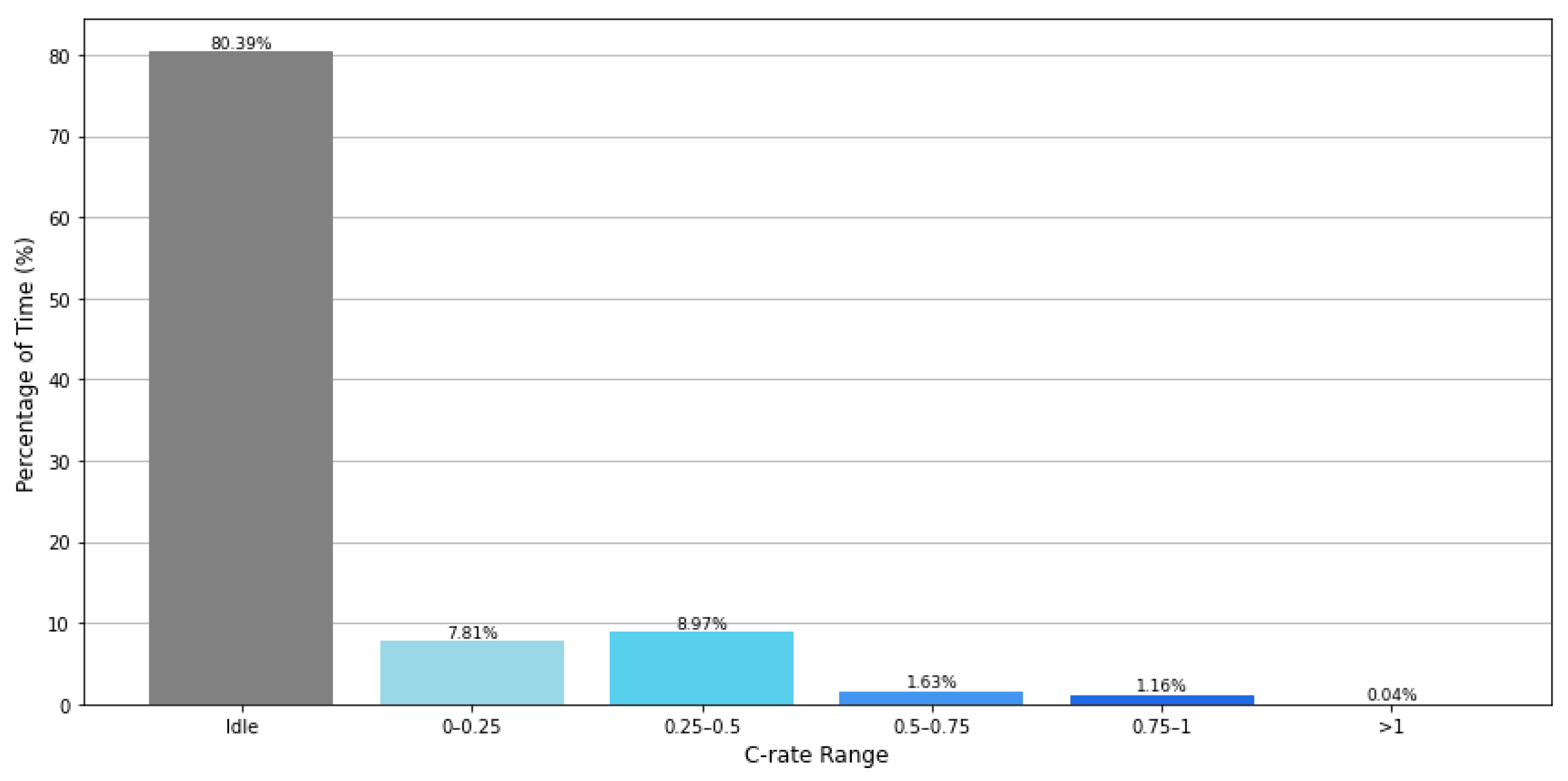
The spreadsheet data indicates that the maximum achievable C-rate is 1.67, which is relatively high for a grid-scale BESS. This suggests that the utilization would occur either in longer durations with a more limited C-rate, or shorter periods at higher C-rates. Thus, to better understand the utilization patterns, an initial analysis was conducted by classifying operation in six groups based on the C-rate levels. Interestingly, it was discovered that the BESS was in idle for 80.39% of the time, and was, in any case, operated with a C-rate lower than 0.5 for 97.17% of the time, and almost never surpassing 1 (Figure 3). These operating conditions, together with the relatively high average temperatures reported in Figure 2, correspond to the scenario identified in [11] as most sensitive to auxiliary consumption, where dedicated modeling is needed to avoid errors in the overall efficiency estimation. This by itself suggests that the heating due to BESS utilization is likely not the sole driving factor of the auxiliaries. We then excluded any timestamps with a C-rate above 1. These made up just 0.04% of the observation period, which is roughly four hours across the full thirteen months. We opted to drop them for two specific reasons. First, because few samples at such extreme utilization rates would end up in their own thinly populated LUT bins, adding little that the model could learn from, while congesting the available resolution for the far more common operating conditions. Second, because their share is so small, removing them barely shifts the distribution of the training or testing sets, both of which still reflect how the asset actually operates.

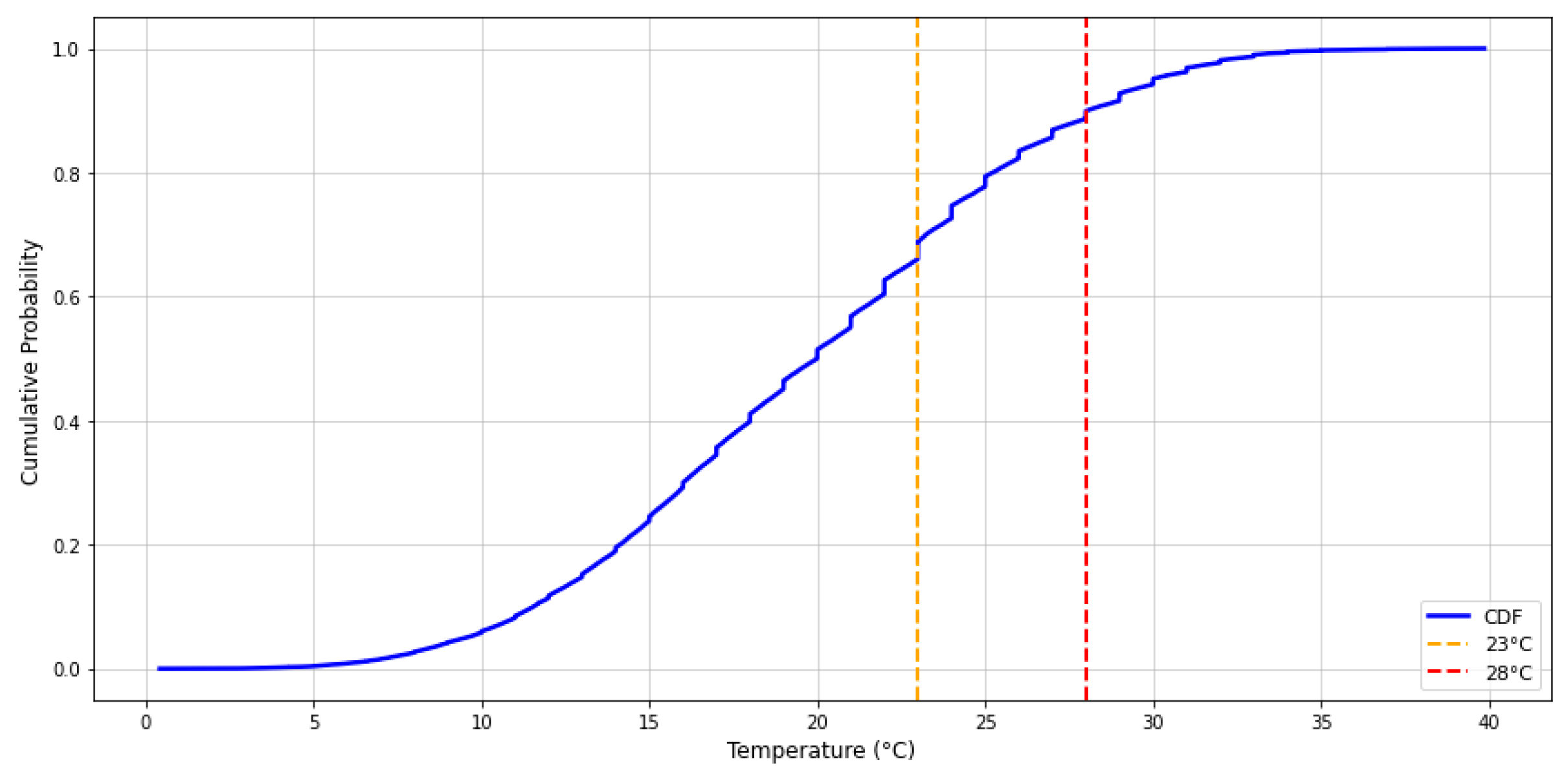
Next, the ambient temperature was investigated, always keeping in mind the setting of the cooling systems that was previously introduced. Indeed, looking at Figure 4 that presents the Cumulative Distribution Function (CDF) of the temperature for the period under investigation, it can be seen that the ambient temperature can be a more significant factor. For each value on the horizontal axis, the curve gives the fraction of time the ambient temperature stayed at or below it, which lets us read off directly how often the cooling thresholds were exceeded. The ambient temperature surpassed 23 °C for 31.9% of the time and 28 °C for 10.3% of the time, suggesting that the cooling system would need to be active even without the presence of additional operational heating.

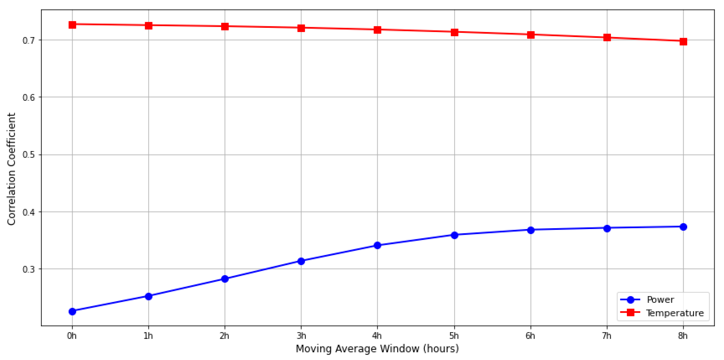
Based on the hypothesis that thermal inertia is a significant factor influencing the instantaneous consumption of the auxiliaries, a statistical analysis was conducted to investigate the Pearson (linear) correlation between the auxiliary load and the moving averages of the predicting variables. The analysis displayed on Figure 5, where the horizontal axis is the length of the moving average and the vertical axis the resulting Pearson correlation coefficient, shows that the ambient temperature exhibits a significantly stronger correlation to the auxiliary consumption compared to the power output. Moreover, the correlation decreases as the temperature moving-average window increases, whereas, for power, the opposite trend is true.

Even though the absolute value of the correlation may be guided by the low utilization rate of the BESS, the behavior of the moving averages hints at very important notion regarding the thermal inertia. In fact, the impact of the ambient temperature seems to have a much lower time constant, directly affecting the temperature inside the container and, thus, the need for cooling. On the other hand, the power output of the BESS seems to have a much more lasting effect, where the correlation visually increases up to a moving-average window of 6 h. Practically speaking, this implies that the impact of the heating caused by the operation of the BESS persists for a longer duration. It should be clarified that this provides only a direction for further analysis, as it is clear that the actual correlation is not linear.

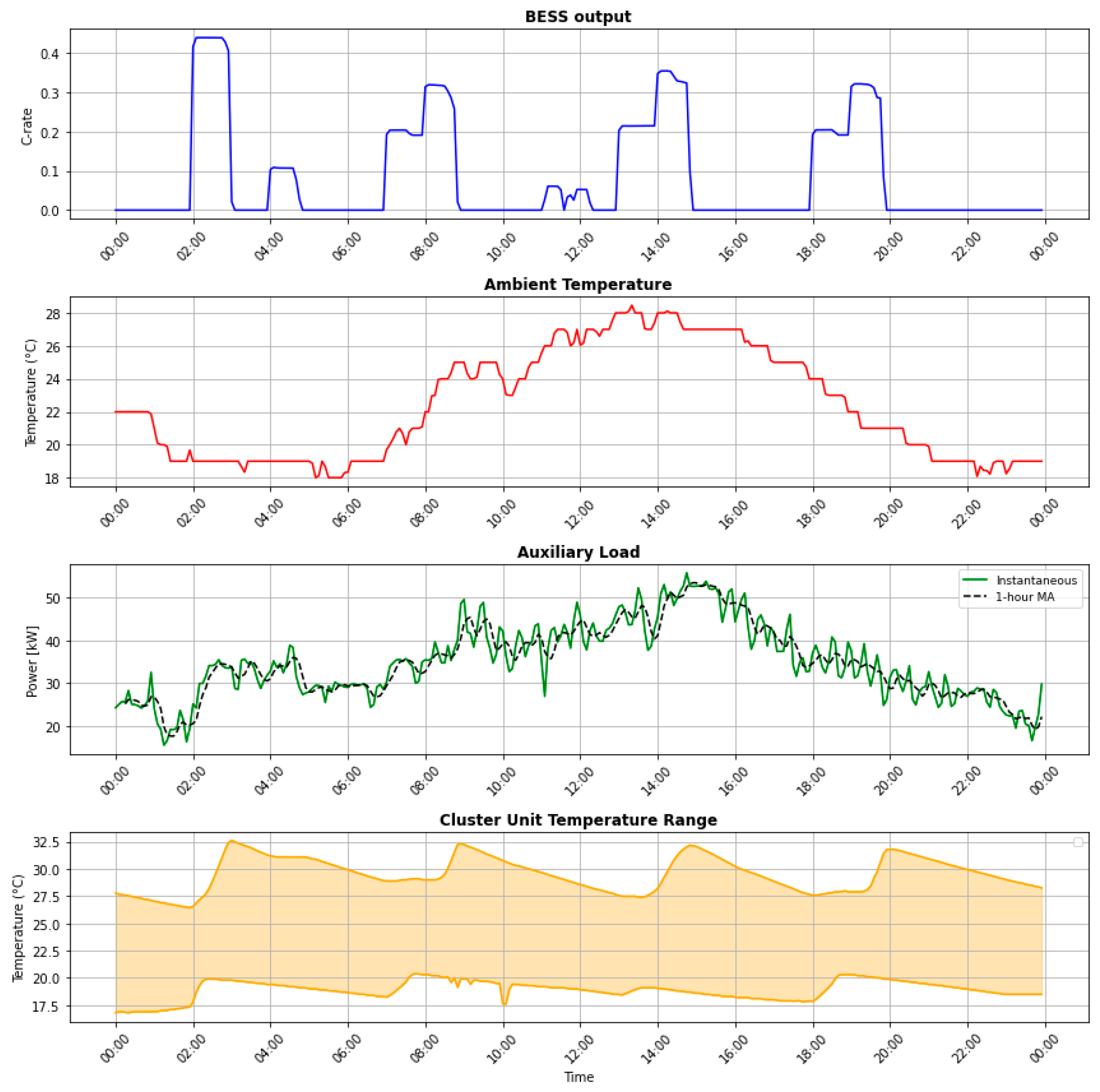
The behavior described above can also be illustrated using a specific example presented on Figure 6, where the BESS power output, ambient temperature, and auxiliary consumption are visualized for a relatively warm day in October. To better capture the underlying trend in auxiliary consumption, a 1 h MA is applied to reduce the effect of the on/off cycling of the auxiliary systems. In addition, temperature measurements inside the containers are recorded as a supplementary plot, providing insights into the thermal dynamics of the containers.

First, a clear relationship can be observed between ambient temperature and auxiliary consumption, particularly when the ambient temperature exceeds the activation thresholds of the cooling system. Moreover, Figure 6 also highlights the asymmetric thermal behavior of the container. Heating occurs relatively quickly due to the coupled impact of BESS utilization and higher ambient temperatures, whereas the subsequent cooling phase takes considerably longer. This difference in the thermal behavior clearly demonstrates that the system could not be adequately described by a single characteristic time constant as the containers exhibit operating-dependent time-constant-like behavior. This notion is examined numerically below. This is something that makes the forecast of the auxiliary consumption required to maintain normal temperature rather challenging, as it complicates the correlations and dependencies between the variables. Clearly, this emphasizes the limitations of relying only on instantaneous variables to characterize the auxiliary consumption.

To complement the qualitative discussion above with a quantitative estimate, the cooling consumption was modeled as a first-order dynamic response toward an equilibrium value determined by the operating conditions. The equilibrium auxiliary consumption P_aux,eq is taken as a function of the absolute BESS power (P_BESS,abs) and the ambient temperature, and its temporal evolution is described by Equations (1) and (2), where β is the fraction of the gap between the current and equilibrium consumption recovered within one sampling interval. In practice, the two relations were combined into a single one-step-ahead expression, in which the auxiliary consumption at the following interval is a linear function of its current value, the absolute BESS power, and the ambient temperature. This expression was fitted by linear regression on consecutive measurements: the coefficient associated with the current consumption yields the relaxation parameter β, while the remaining coefficients recover the equilibrium relationship of Equation (1). Converting β to an equivalent thermal time constant (τ) through Equation (3) yields a characteristic response time of approximately 29 min. The linear identification is used here solely to extract the characteristic relaxation timescale, and not as a predictive model of auxiliary consumption; consistent with the non-linear behavior discussed above, its role is to quantify the response time rather than to replace the data-driven models developed in the following sections.

$${\mathrm{P}}_{\mathrm{a}\mathrm{u}\mathrm{x},\mathrm{e}\mathrm{q}}=\mathrm{f}({\mathrm{P}}_{\mathrm{B}\mathrm{E}\mathrm{S}\mathrm{S},\mathrm{a}\mathrm{b}\mathrm{s}},{\mathrm{T}}_{\mathrm{a}\mathrm{m}\mathrm{b}})$$

(1)

$${\mathrm{P}}_{\mathrm{a}\mathrm{u}\mathrm{x}}\left(\mathrm{k}+1\right)={\mathrm{P}}_{\mathrm{a}\mathrm{u}\mathrm{x}}\left(\mathrm{k}\right)+\mathsf{\beta }({\mathrm{P}}_{\mathrm{a}\mathrm{u}\mathrm{x},\mathrm{e}\mathrm{q}}\left(\mathrm{k}\right)-{\mathrm{P}}_{\mathrm{a}\mathrm{u}\mathrm{x}}\left(\mathrm{k}\right))$$

(2)

$$\mathsf{\tau }={\displaystyle \raisebox{1ex}{$∆\mathrm{t}$}\!\left/ \!\raisebox{-1ex}{$\mathrm{l}\mathrm{n}(1-\mathsf{\beta })$}\right.}$$

(3)

This value should be interpreted with care. As the asset is idle for the large majority of the observation period, the estimate is dominated by transitions occurring under quiescent conditions, and, therefore, reflects the relatively fast relaxation of the cooling system toward its immediate equilibrium rather than a single time constant valid across all operating regimes. During and after active power provision, the effective response is considerably slower, as the operational heat propagates through the thermal mass and sustains the cooling demand well beyond the immediate interval—consistent with the multi-hour influence of BESS power observed in the moving-average correlation analysis (Figure 5). The two observations are complementary: the short response time characterizes how quickly the cooling system tracks its equilibrium, while the long moving-average dependence characterizes how long operational heat perturbs that equilibrium. Taken together, they confirm that the system cannot be adequately represented by a single characteristic time constant, and they provide a data-driven justification for the use of multiple moving-average windows—a short one to capture the fast thermal response and longer ones to capture the persistent effect of prior operation.

Instead, the use of moving-average predictors could provide a more appropriate representation of the thermal processes. As can be seen from the example, the auxiliary systems remain active long after the BESS utilization that generated the heat. This effect is particularly clear following the service interval between 02:00 and 03:00 (Figure 6), where a period of relatively high C-rate operation leads to a gradual increase in auxiliary consumption. It then remains elevated for a longer period, even though the ambient temperature remains relatively low, whereas the temperatures inside the container gradually decrease.

The sections below summarize the different approaches investigated. In all the cases, the available dataset is first split between training and testing, using the random 80–20 split, in order to enable an unbiased evaluation of the models’ generalization performance and allow for an equal-ground comparison among them. The main performance evaluation metric to assess model accuracy is the Root Mean Square Error (RMSE), a well-established evaluation metric in the field as it penalizes larger prediction errors and provides a direction-independent measure of model performance. Finally, to complement the comparison along the models, the Mean Absolute Error (MAE) is also computed, as it penalizes all errors linearly, thereby improving outcome interpretability and providing a measure of typical operational accuracy.

3.4. 2-Dimensional Look-Up Table (LUT) Taken from the Literature

This section briefly summarizes the approach proposed by the authors in [10], utilized as a literature reference for evaluation of the results. It is based on the creation of a 2-dimensional LUT utilizing BESS power and ambient temperature as predictors. For each dimension, the range between the minimum and maximum observed values is evenly divided using eight breakpoints to create the bins. Then, the values of the lookup table at each grid point are computed as the average of the data within the corresponding bin. Similarly, data samples within each bin are averaged to compute the corresponding auxiliary consumption. In the LUT obtained, each bin is represented by the average value on each of the two dimensions. The LUT evaluation is then performed using linear interpolation between the nearest grid points for each data sample in the testing dataset.

3.5. 3-Dimensional Look-Up Table (LUT)

Given the correlation discovered in the exploratory analysis that showed high importance of the power moving average, the first approach proposed by this paper to building a model is to propose a more detailed LUT that can be used to estimate the auxiliary consumption. In this case, the idea is to go one step further from the 2-D LUT approach proposed by the literature [10] and briefly explained in Section 3.1, and propose a 3-D LUT that, on top of the instantaneous power and ambient temperature, incorporates a selected moving average of the power with a duration h hours MA(P_BESS, h). This selection is motivated by the findings of the exploratory analysis performed using the Pearson correlation shown in Figure 5, which indicates not only a correlation between the power moving average and auxiliary consumption, but also that the correlation increases with the duration (h) of the moving average. On top of it, the approach does not fix the number of breakpoints, but, instead, allows the algorithm to search for a well-performing configuration. Algorithm 1 presents a step-by-step pseudocode description of the proposed procedure.

Algorithm 1. Monte Carlo approach for the creation of a 3-D lookup table

Input: PBESS—power time series; Tamb—temperature time series; PAUX—auxiliary consumption time series; NMA—max BESS power MA window [h]; NBP—max possible breakpoints per dimension ITMAX—max iterations; ε—convergence criterion [iterations without improvement] Output: Best configuration: lookup table (LUT*), RMSE*

1:     Construct feature set: F ←{PBESS, Tamb} 2:     Append MA of PBESS: {MA(PBESS, k): k = 1 … NMA} to F 3:     Append PAUX to obtain the dataset and split in training/testing: DTRAIN, DTEST ←{F, PAUX} 4:     Initialize parameters: RMSE* ← ∞; counterNoImprove ← 0; counteriterations ← 0; LUT* ← ∅

5:     while counter < ε and it < ITMAX do: 6:       Sample number of breakpoints: nBP,Pbess,, nBP,Tamb, nBP,MA ~ U{3, …, NBP} 7:       Sample MA window: h ~ U{1, …, NMA} 8:       Define the set of three dimensions D {PBESS, MA(PBESS,h), Tamb} 9:       Sample breakpoints for each d ∈ D: BPS,d ← (nd − 2) interior values ~ U(mind, maxd) 10:       Set the breakpoints vector for each d ∈ D: BPd ← {mind} ∪ {BPS,d} ∪ {maxd} 11:       Split training dataset (DTRAIN) in each bin (i, j, k) defined by the breakpoints BPd → DI,J,K 12:       Calculate LUT value for each bin: LUT[i, j, k] ← mean(PAUX ∈ DI,J,K) 13:       Query LUT and calculate auxiliary load using linear interpolation of the closest BPs: → $\hat{\mathrm{P}}$AUX 14:       Evaluate RMSE on testing dataset: → RMSE = RMSE(PAUX, $\hat{\mathrm{P}}$AUX) 15:       if RMSEIT < RMSE* then: 16:         RMSE* ← RMSEIT; LUT* ← LUT; counterNoImprove ← 0 17:       else 18:         counterNoImprove ← counterNoImprove + 1 19:       end if 20:       it ← it + 1 21:     end while

22:     return LUT*,  RMSE*

The developed framework is a probabilistic Monte Carlo grid-based non-parametric estimator. As one of its main features, it does not require the fixing of its discretization structure a priori. Instead, a stochastic sampling procedure was employed to explore different partition granularities. For each iteration until convergence is reached, the moving-average window length (h) for the power of the battery MA(P_BESS, h), and the number of breakpoints per predictor (n_BP,Pbess,, n_BP,Tamb, n_BP,MA) were randomly sampled from predefined uniform distributions. The allowed values are ranging from three up to a predefined maximum (N_BP). In this way, the approach targets a good break-point configuration with a probabilistic criterion. Given the sampled breakpoint count, partition boundaries were constructed across the observed variable range, respecting the minimum and maximum values for each predictor, resulting in a candidate three-dimensional grid. Each cell of the grid represents a specific combination of intervals for each of the three predictor variables. Then, the auxiliary consumption associated with each cell was computed as the average of all samples falling within the corresponding parameter ranges.

Once the LUT is created, its performance is evaluated using the testing dataset. For each observation, the corresponding region in the three-dimensional predictor space was identified, and the auxiliary consumption was estimated with a linear interpolation between adjacent grid cells. The LUT configuration achieving the lowest RMSE is then selected as the final model for the 3-Dimensional LUT approach.

3.6. Random Forest Regression

In addition to the grid-based 3-D LUT approach, a machine-learning method based on RF was also evaluated. RF is an ensemble learning method that builds a large number of decision trees using bootstrap resampling of the training data and random subsets of predictor variables at each split. Practically speaking, each tree is built using different subsets of the training data and predictor variables. The final prediction is obtained by averaging the outputs of the individual trees. This practice of combining bootstrap aggregation with random feature selection reduces variance and mitigates overfitting, effectively improving generalization. This is done while preserving the ability of decision trees to model complex non-linear relationships between the predictors and target variable. Unlike the LUT approach which relies on explicit discretization of the predictor space into predefined grid cells, RF performs recursive partitioning of the search space. Owing to this underlying feature, it can capture the non-linear interactions between the instantaneous temperature and power, alongside their different moving averages, without requiring manual selection of breakpoints or dimensionality constraints.

Indeed, one of the limitations of the LUT concept is the dimensionality, since, by adding predictors such as multiple moving-average horizons, the number of grid-cells would grow exponentially, leading to very sparsely populated regions and unreliable estimates. Thus, only a limited number of dimensions can be included while maintaining sufficient samples per cell. Indeed, the approach proposed considered only three dimensions, one of which was a uniformly selected time horizon of the power moving average. On the opposite, RF is not subject to this restriction in the same way. Because splits are created adaptively and the algorithm can select which predictors are the best to use, the method can incorporate multiple moving-average features simultaneously without requiring explicit binning. On top of it, it removes the need to select a single “best” moving-average window to be used for forecasting purposes, allowing the model to internally determine the relative importance of different windows.

Even though the RF algorithm involves several hyperparameters such as the number of trees, maximum tree depth, and minimum samples per leaf, the tuning of these parameters was considered outside of scope of this paper. The main rationale is that, in limited datasets, the impact on these parameters is very modest and, thus, default values from the literature can be adopted [22]. As introduced before, the key indicator used during training and evaluation was the RMSE.

In order to systematically evaluate these advantages over the LUT-based approaches, as well as find the best trade-off in terms of model expansion, a hierarchical feature-addition framework was adopted. It adopts a brute-force strategy to assess the impact of adding calculated predictors in the form of moving averages on the performance metrics. The incremental addition of predictors enables the evaluation of whether increasing feature complexity improves performance, or, beyond a certain point, begins to degrade it. The procedure is summarized in a high-level pseudocode in Algorithm 2.

Algorithm 2. Random Forest Moving-Average window search

Input: PBESS—power time series; Tamb—ambient temperature time series; PAUX—auxiliary consumption time series; Np—max BESS power MA window [h]; Nt—max temperature MA window [h]; TBOOL—consider instantaneous temperature Output: Best RMSE value (RMSE*) and corresponding configuration (np*, nt*)

1:     for np = 0 to Np do: 2:       Construct feature set: Fp ← {PBESS} 3:       if np > 0 then: 4:         Append power MA to F: Fp ← Fp ∪ {MA(PBESS, k): k = 1 … np} to Fp 5:       end if 6:       for nt = 0 to Nt do: 7:         if TBOOL then: 8:             Update feature set: F ← Fp ∪ {Tamb} 9:         else: 10:             Update feature set: F ← Fp 11:         end if 12:         if nt > 0 then: 13:              Append {MA(Tamb, k): k = 1 … nt} to F 14:         end if 15:         Train/test split: FTRAIN, FTEST ←F 16:         Train Random Forest on feature matrix X built from FTRAIN → RF(FTRAIN) 17:         Evaluate auxiliary consumption for the testing dataset: $\hat{\mathrm{P}}$AUX ← RF(FTEST) 18:         Evaluate RMSE on testing dataset: → RMSE = RMSE(PAUX, $\hat{\mathrm{P}}$AUX) 19:         if RMSE < RMSE* then: 20:              RMSE* ← ε; best_config* ← (np*, nt*) 21:         end if 22:       end for 23:     end for

24:     return RMSE*, config*

Similarly to the LUT-based approaches, the analysis was structured along two dimensions, ambient temperature and BESS power. In the outer layer, the predictors related to the temperature are progressively expanded, starting from instantaneous temperature and incorporating moving-average features with increasing window lengths, each time adding one hour. Practically speaking, Algorithm 2 needs to be executed once without the instantaneous temperature, and then iterate the different moving averages, controlled with the Boolean T_BOOL. For each temperature configuration, an inner cycle is performed in which power moving-average predictors are incrementally added, adding one hour to the moving-average calculation per iteration. Essentially, it can be visualized as a nested “for” cycle, where the temperature is the upper level.

This nested evaluation strategy enables an organized evaluation of the combined effects of power and temperature on the thermal inertia of the system, effectively evaluating the time constants associated. In this way, the framework not only facilitates a direct performance with the LUT-based approaches, but also provides a structured assessment of how accuracy is impacted when additional temporal information is included.

Finally, to simulate realistic operational conditions, the trained estimator was also tested under a persistence-based temperature forecasting scenario. In the testing dataset, ambient temperature inputs were replaced with the corresponding values from the previous day, therefore simulating forecasting uncertainty. This approach is particularly relevant for potential day-ahead scheduling applications where, even though the power dispatch profile is generally known in advance, temperature can only be forecasted. The persistence model forecast is a well-documented and acceptable approach especially for the case of temperatures, given that day-to-day variations are nonetheless quite limited on average. Therefore, this analysis should be interpreted as a robustness test for the proposed approach in the absence of temperature forecasting information, where temperature forecast errors may vary. It is worth noting, however, that persistence forecasting is generally regarded as a conservative baseline, since a dedicated forecast service would typically outperform it. Therefore, the increase in prediction error obtained here is not expected to be a systematic underestimate of the impact of temperature forecasting. Accordingly, this analysis should be read as a robustness test of the proposed approach under imperfect temperature information, providing only an indicative rather than exact quantification of the impact of forecast uncertainty.

4. Results

The following section introduces the outcomes of the three approaches investigated—the 2-D LUT-based approach adapted from the literature, alongside the 3-D LUT-based and RF-based frameworks proposed by this paper. Each approach is analyzed separately to emphasize its performance and main characteristics, and address its limitations. To provide a reference for the computational effort indicators reported below, the simulations were performed on a Windows machine equipped with a 12th Generation Intel Core i7-1260P processor, integrated UHD Graphics Card, and 16 GB of RAM.

4.1. 2-Dimensional LUT Outcome

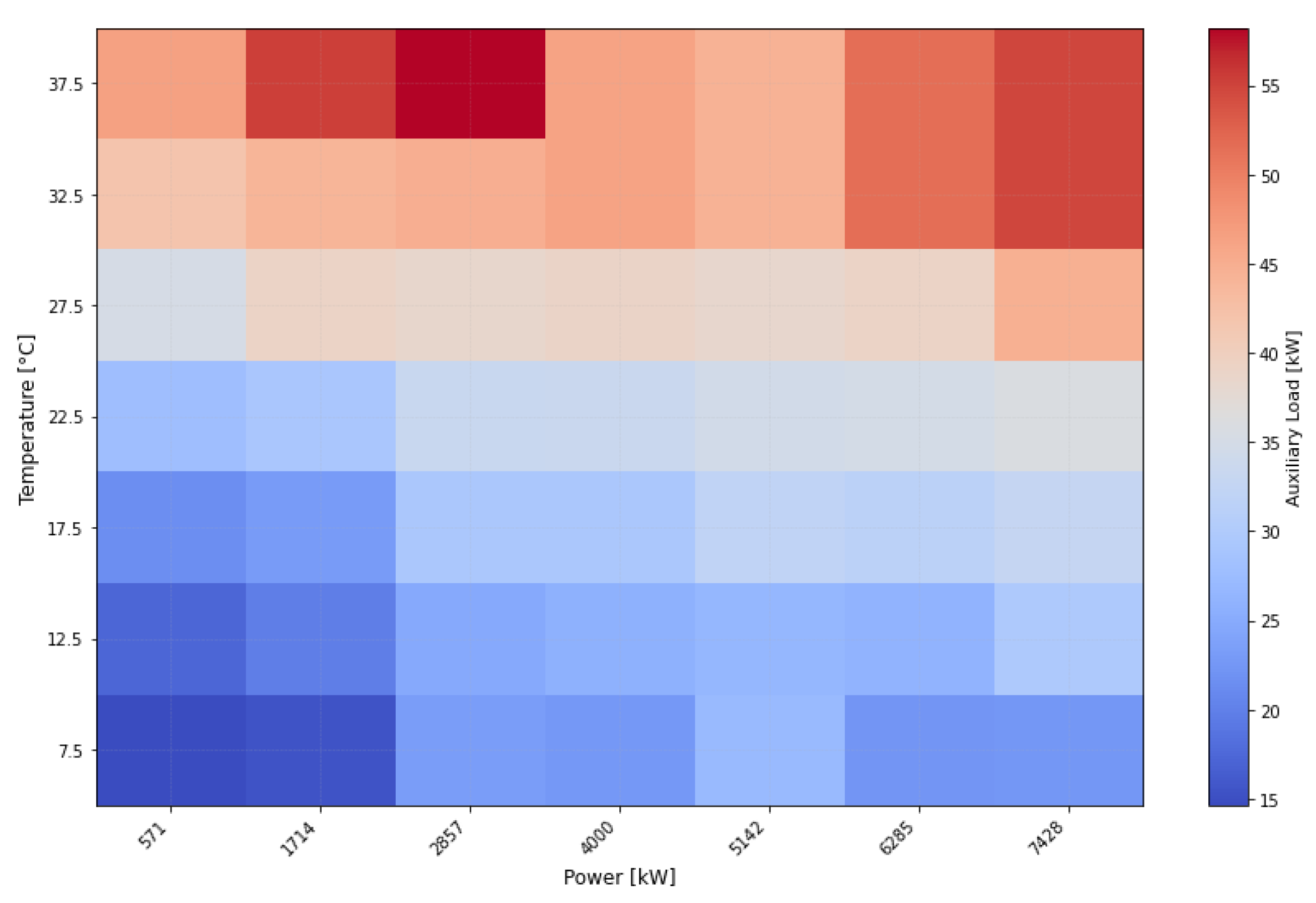
The LUT obtained with the approach proposed by the literature [10] is provided as a heatmap on Figure 7. The model achieved an RMSE of 6.81 kW, which is 9.4% of the maximum recorded auxiliary consumption, and 23.4% of the mean.

Even though the approach is clearly able to decently capture a correlation between temperature and auxiliary consumption, evidenced from the increasing values along the y-axis, it fails to accurately represent the correlation with the BESS utilization. For example, the model obtained suggests that a low utilization of the BESS at high temperature results in a lower cooling demand than higher power operation, something that does not reflect the real thermal dynamics of the system. Nevertheless, the approach can certainly provide a reasonable first estimate, especially during prolonged idle times when clearly the main driving factor would be the ambient temperature. Given the characteristics of the dataset, particularly the high proportion of idle operation, the resulting RMSE can be seen as acceptable. However, a more in-depth analysis enabled by Figure 7 shows that the model is far from capturing the true thermal dynamics and the dependency of the auxiliary consumption on BESS utilization. The computational complexity in this case is negligible, as the LUT is obtained with a one-shot processing of the data.

To examine whether the baseline error concentrates in specific operating regimes, the RMSE of the 2-D LUT was computed per bin of the temperature–power grid. It was found that, in absolute terms, the error grows with both temperature and power, ranging from approximately 3.2 kW in the idle and low-power bins, to 10.8 kW at the highest power and near-highest temperature. This trend, however, is affected by the higher auxiliary consumption in those conditions: once the per-bin RMSE is normalized by the average auxiliary consumption of each bin, the values are more dispersed (between 0.16 and 0.28) and show no clear dependence on the operating conditions.

4.2. 3-Dimensional LUT Outcome

The LUT algorithm was executed with a threshold of maximum 10,000 iterations (IT_MAX), with the stopping criterion (ε) of 500 consecutive iterations without an improvement in the RMSE metric. These relatively large limits were chosen to ensure a robust search of the solution space. The maximum number of breakpoints (N_BP) for each predictor was set to 10, while, as previously described, the actual breakpoint values were constrained by the observed minimum and maximum values for each predictor, respectively. The maximum moving-average window (N_MA) used for the power calculation was set to extend up to 8 h.

The LUT that provided the best representation of auxiliary consumption corresponded with a 5 h moving average, emphasizing the dominant influence of the longer time constant of power on auxiliary consumption. In the best-performing configuration, the algorithm selected five breakpoints for the instantaneous power, nine breakpoints for the instantaneous temperature, and nine breakpoints for the 5 h moving average to best capture the correlation structure. This outcome further supports the initial hypothesis that the moving-average power is more relevant than the instantaneous value, as it better captures the complex thermal effects within the container. More specifically, the combination of the instantaneous power with a longer moving average reflects the two-timescale nature of the cooling response identified in Section 3.2: the instantaneous power captures the fast component of the thermal response, characterized by the short equilibrium relaxation time, while the 5 h moving average accounts for the slower, persistent effect of the prior operation on the container temperature. The predictor structure selected by the algorithm is, therefore, consistent with the underlying thermal dynamics, rather than being a purely data-driven artifact. In terms of the computational complexity, the solution took a total of 1190 iterations and 325 s to converge.

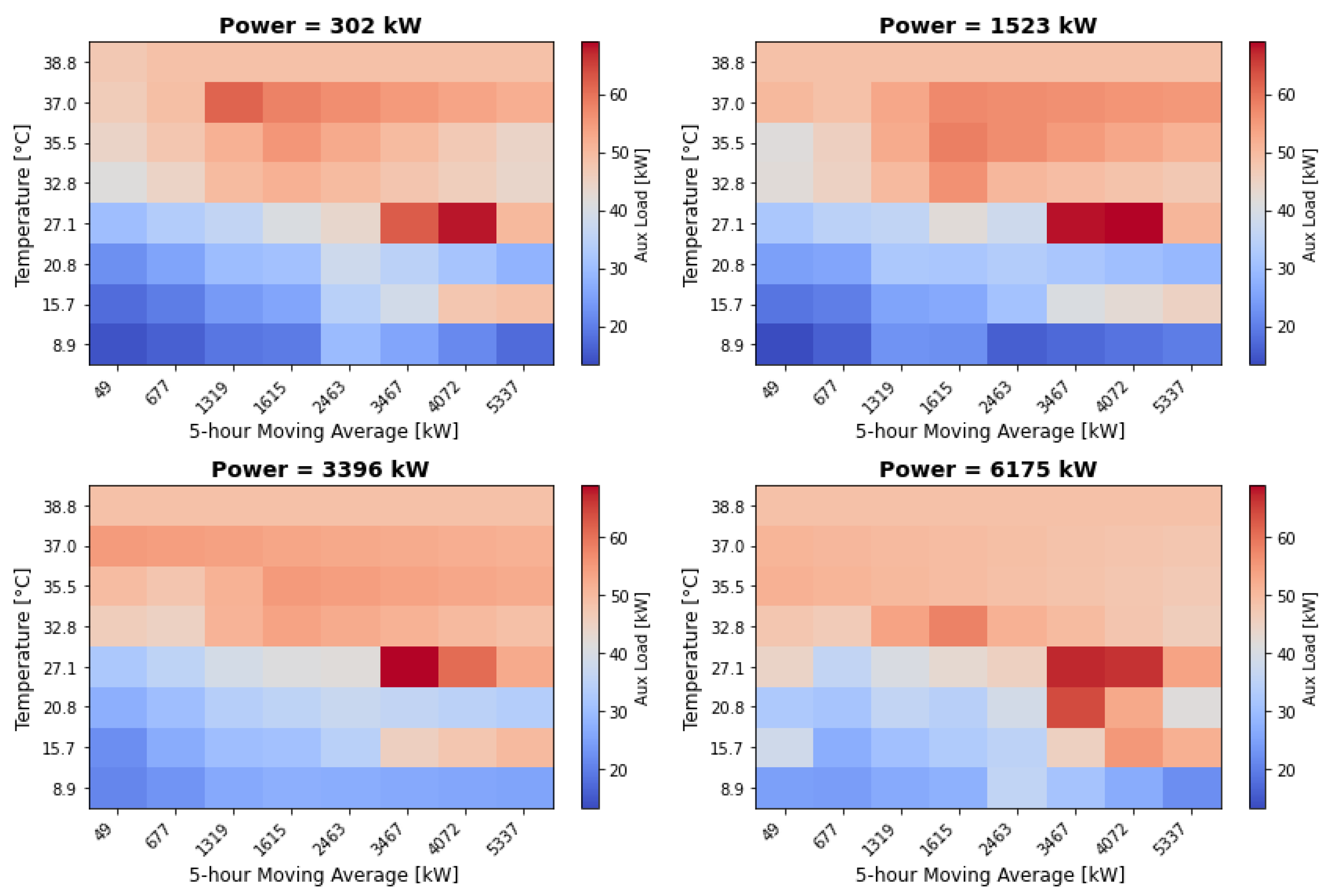
The higher dimensionality of the LUT complicates the visualization and interpretation of the outcome, so, to best address this issue, one dimension is represented through multiple subplots, while the remaining two are displayed using heatmaps. In line with the structure of the solution, four subplots were provided for the instantaneous power, with the moving-average power and the ambient temperature provided on the two axes. Figure 8 demonstrates the resulting breakpoints, the associated bins, and the average auxiliary consumption associated with each breakpoint.

Applying the LUT to the testing dataset, the predicted auxiliary consumption achieved an RMSE of 5.32 kW, indicating a reasonably accurate estimation of the system behavior. In relative terms, this represents 7.4% with respect to the maximum auxiliary consumption, and 18.3% with respect to the mean. Nevertheless, considering the much larger size of the BESS itself, this outcome can be seen as very prominent for practical applications. Looking at Figure 8, it can be seen that the LUT approach was able to capture the operational characteristics of the BESS plant, which is typically operated at a lower C-rate (Figure 3). Indeed, we can see that the breakpoints both on the instantaneous and moving-average power are on the lower side of the 14.7 MW rated power of the plant. On the other hand, the breakpoints for the temperature spread wider across the different operational conditions.

In terms of auxiliary load estimation, it is clear that it has a positive, but not exactly linear, correlation with the predictor variables, which was expected. For example, we can see that, at lower ambient temperatures, the power output of the BESS has a minor impact on auxiliary consumption, as it takes more time to arrive at a temperature inside the container that requires the activation of the HVAC systems. At the same time, Figure 8 provides insights into the imperfections and areas where the approach falls short. For example, the breakpoint defined by T_amb = 27.1 °C and MA(P_BESS, 5) = 3467 kW is a particularly strange case, where, based on the solution, the auxiliary consumption for an instantaneous power of P_BESS = 3396 kW seems to be higher than the one for the P_BESS = 6175 kW. Nevertheless, this can and should be interpreted as not an issue of the approach itself, but simply an issue of dimensionality and insufficient data to train the model with. It also clarifies that going beyond the three-dimensionality of the problem and the limitations in terms of the breakpoints’ threshold would not only be impractical, but would most likely reduce performance.

4.3. Random Forest Regression Outcome

The RF framework introduced in detail in Algorithm 2 was applied to the same dataset, as it enables an equal-grounds comparison. The analysis focuses not only on its predictive accuracy, but also the influence of the addition of calculated predictors, as well as its ability to better represent the complex relationships between the parameters that the LUT approach may have failed to capture.

In terms of setup parameters, similar to the case for the LUT approach, the maximum number of moving averages to be added for the power (N_p) was set to eight hours. However, this number was reduced for the temperature (N_t), as, from the exploratory analysis, it was clear that the impact of the ambient temperature is significantly more instantaneous compared to the impact of the power. Thus, this step was taken to avoid redundant iterations and avoid potentially over-fitting the model without a physical meaning. The training of the models took between 6 s for the case with only 2 predictors, up to 55 s for the case with 13 predictors, whereas the entire hierarchical feature-addition framework took a total of 1540 s. The training and testing of the RF model was performed by using the scikit-learn library (version 1.6.1) in python.

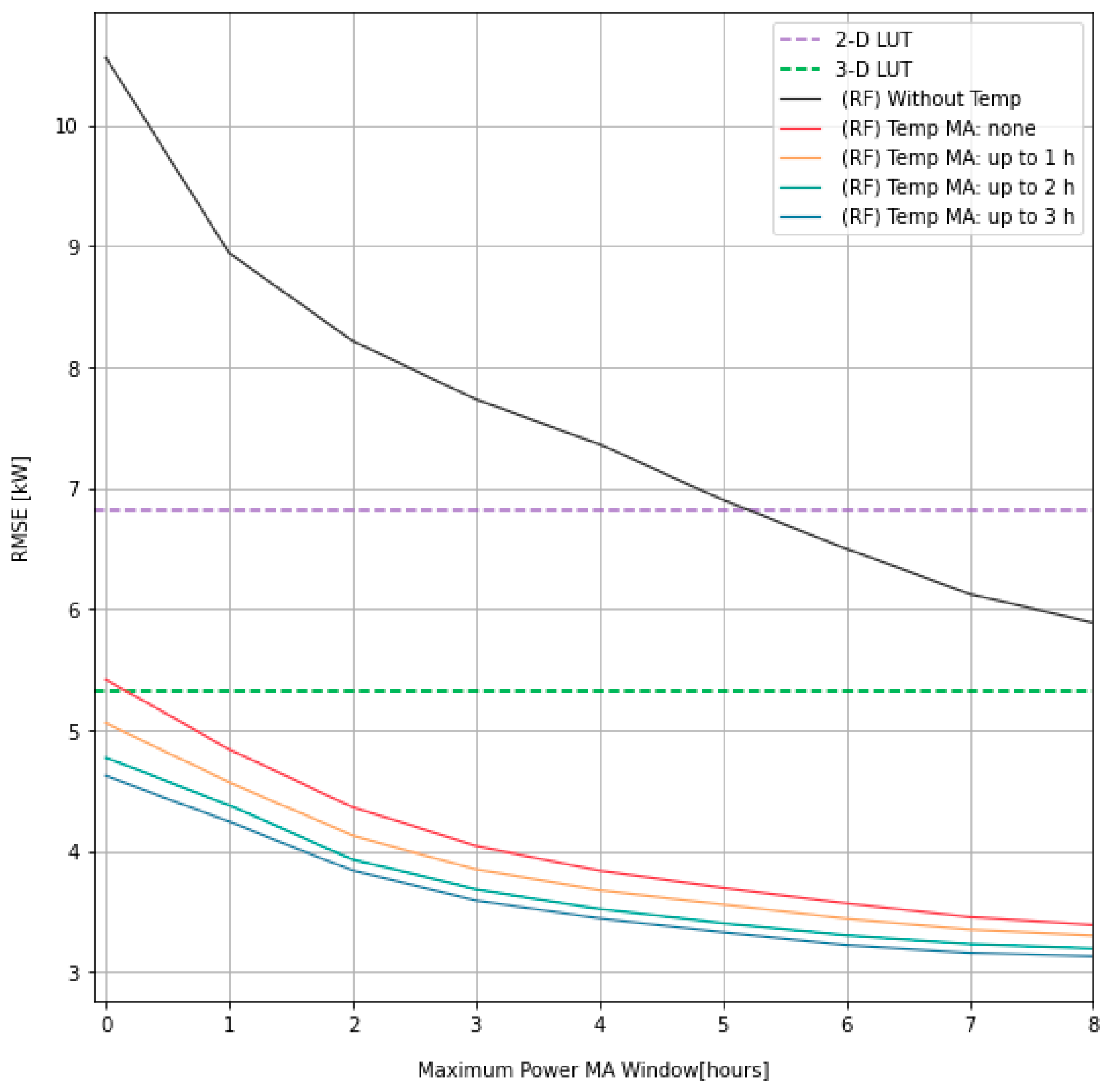
The outcome of the recursive addition of moving-average predictors is presented on Figure 9, alongside a comparison with the values obtained from the LUT-based approaches. Moreover, it should be clarified that the x-axis represents the “up-to” power moving average added. For example, the value of 3 signifies that the 1 h, 2 h, and 3 h moving averages have been added as predictors. For clarity, from this moment on, a moving average of 0 represents simply the instantaneous value.

For clarity, it should be noted that the black line (“Without temp”) represents the results obtained by executing Algorithm 2 with T_BOOL = False, whereas the rest are obtained with T_BOOL = True. In order to provide a more effective comparison with the LUT-based approaches, their performances are added on Figure 9. The main outcome of the analysis is the best configuration for the RF model, and, looking at Figure 9. it is clear that the best outcome is achieved by including the maximum number of predictors, up to 8 h of the power moving average, and up to 3 h of the temperature moving average, achieving an RMSE of 3.13 kW. Obviously, this is a significant improvement of 41.1% over the 3-D LUT approach; however, in absolute terms, the practical impact could be limited. Notably, configurations including the ambient temperature and at least three predictors, as is the case of the 3-D LUT approach, performed better, which is a testament to RF’s superiority in creating a powerful regressor by accurately modeling complex non-linearities.

A second key interpretation of the results is the effect of the ambient temperature. The separation between the black line (without instantaneous temperature) and red line (with instantaneous temperature) highlights that the main improvement in accuracy is achieved by using the instantaneous ambient temperature as a predictor. Even though adding power moving-averages leads to improvements, the importance is not comparable. For example, using solely the instantaneous power is obviously not sufficient and arrives at an RMSE of 10.55 kW. However, starting from this point and adding a 1 h moving average of the power only improves the RMSE to 8.94 kW, whereas adding solely the instantaneous temperature arrives at 5.42 kW, which is a drastically more significant improvement (Figure 9). Nevertheless, from Figure 9, it is also clear that the further inclusion of temperature moving-averages leads to only minor improvements, with diminishing returns when continuing to add more predictors. Understanding the theoretical background of the RF method, it is clear that this may lead to overfitting. Thus, by examining the shapes of the curves on Figure 9 and searching for the “knee”, it becomes clear that even adding a few power moving averages, together with either just the instantaneous temperature or also the first-hour moving average, could provide adequate performances.

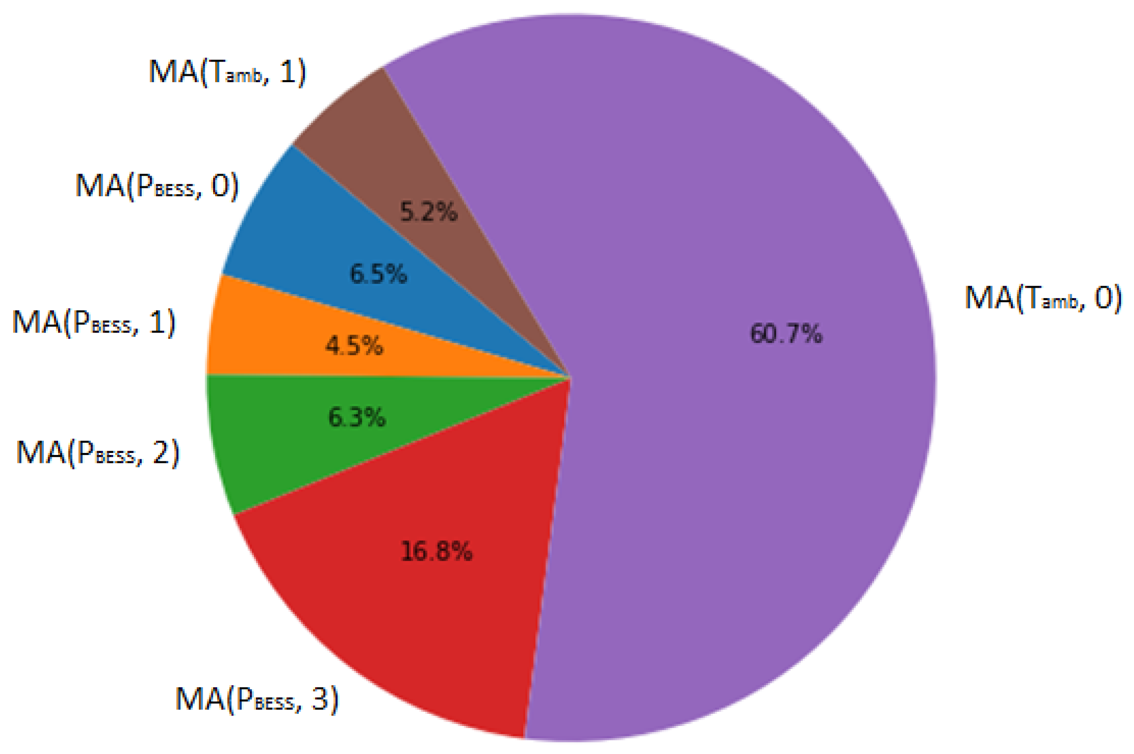
Another metric that can be used to perform the same analysis is the feature importance, or feature utilization of the RF method. Indeed, because the RF prediction consists of many decision trees, features that are frequently used to make informative splits are considered more important, as they tend to reduce the variance in the case of regression. More precisely, the importance of a feature is measured by how much it reduces the prediction variance across all the splits where it is used, normalized so that the values sum to one; a larger value simply means the model leaned on that predictor more. Thus, Figure 10 provides an example of the case with n_p = 3 (or up to 3 h power moving averages) and n_t = 1 (up to 1 h temperature moving average), while also considering the instantaneous temperature as well. The outcome clearly shows the importance of the instantaneous temperature above all, followed by long-lasting moving-average power values to best correlate with the thermal processes and cooling requirements of the containers.

That said, it should be noted that this behavior is definitely impacted by the utilization patterns of the BESS, and is thus a quite specific behavior, as Figure 3 reported more than 80% of idle time. During those times, it is clear that the main driver of auxiliary consumption must be the temperature, as the battery is not utilized and does not heat the container.

Finally, as introduced in the methodology section, the same analysis was repeated by using a modified dataset using a persistence temperature forecast, allowing us to simulate the performance of the approach for day-ahead auxiliary consumption predictions when reliable ambient temperature forecast data are not available. It should be clarified that this modification is only applied to the testing dataset, assuming that the forecast affects the evaluation, whereas the training of the model is performed with known data. The outcome was an average of a 1.13 kW increase in the RMSE in absolute terms, or 30% in relative terms. In the best-case scenario with the maximum number of predictors, the error increased from 3.13 kW to 4.39 kW, effectively introducing the maximum increase of 40% in relative RMSE. With that being said, it should be noted that these values remain within an acceptable range for the practical implementation of these forecasts, supporting the applicability of the approach while acknowledging that a dedicated temperature forecast would refine this estimate.

4.4. Model Comparison and Time-Series Application

This section compares the two approaches proposed against the one proposed in the literature. In terms of the RF, the best performance with the maximum number of predictors will be considered. First,

Table 1. Model performance comparison.

	RMSE [kW]	MAE [kW]
2-D LUT [10]	6.81	4.92
3-D LUT	5.32	4.11
Random Forest	3.13	2.38

summarizes the RMSE and MAE error metrics for the three models investigated.

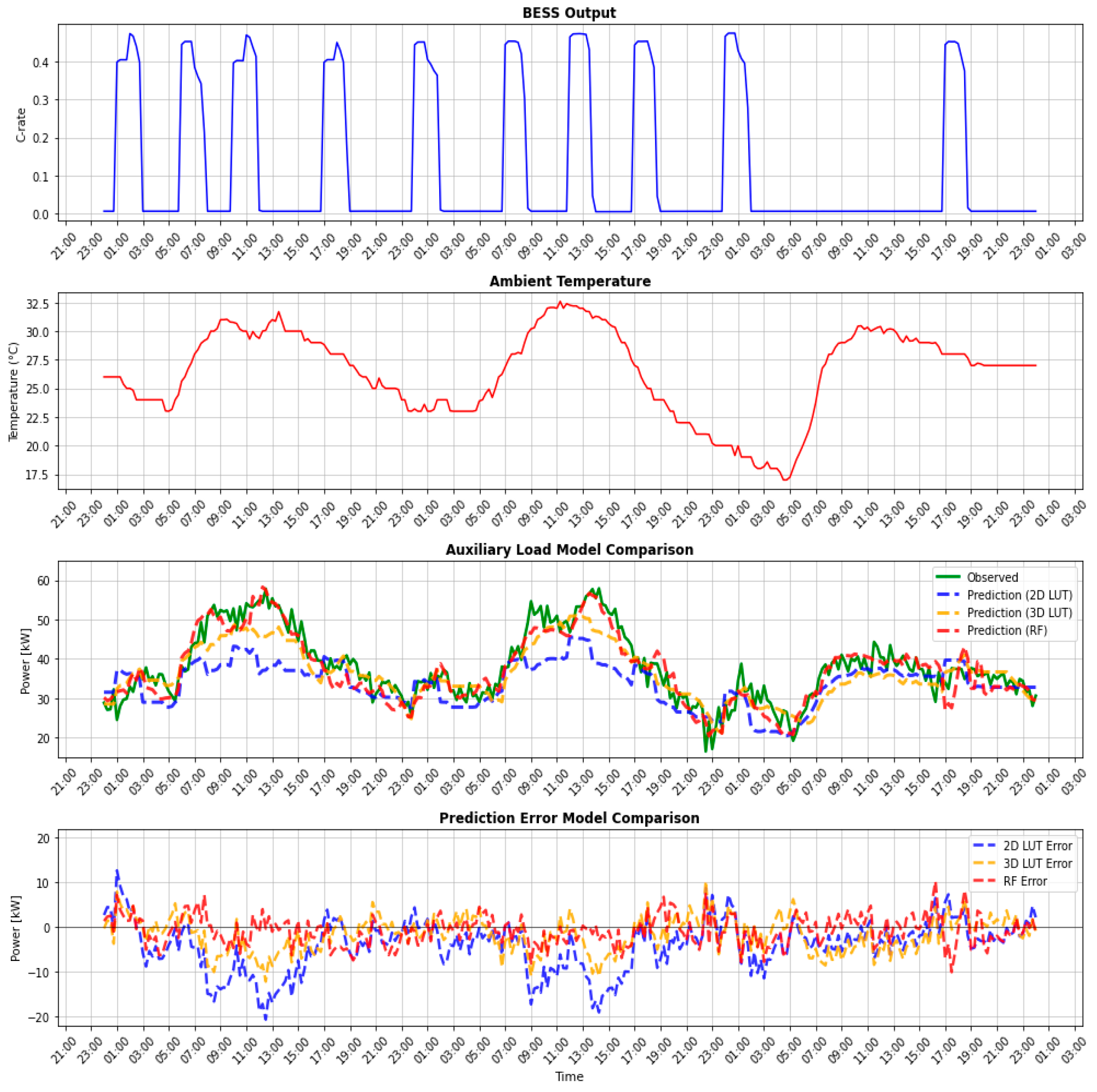
It is evident that the two approaches proposed outperform the 2-D LUT method proposed by the literature by a significant margin. Considering the RMSE as a reference metric, the 3-D LUT approach yields a 21.9% improvement over the literature method, while the RF achieves a significant 54% performance gain. A consistent trend is observed when comparing the MAE, with improvements of 16.4% and 51.6% for the 3-D LUT and RF methods, respectively. Although the computational time is more significant for the two proposed approaches than for the literature LUT, in all cases, it remains well within the time available to the operator in a day-ahead setting, where the models are rebuilt once per day. It, therefore, does not represent a limiting factor in the selection of the model for this application. However, these performance indices alone may not adequately reflect the real implications of the observed performance. This is why the two LUT methods and the trained RF model were applied on a separate three-day interval that was not utilized during the training and testing of the models. The interval selected had frequent operation intervals, allowing for the investigation of the correlation of both main predictors with respect to the auxiliary consumption. The main outcome of the analysis, joined by the time series of the power exchanged by the BESS and ambient temperature over the observed interval are displayed on Figure 11. The upper panels show the BESS power and the ambient temperature over the interval, and the lower panel puts the measured auxiliary consumption side by side with the three model predictions on the same time axis, so each model’s error can be read against the conditions that caused it. This allows for a clear comparison of the different performance of the investigated models, and the superiority of the RF over the LUT-based approaches. The main improvements can be seen once the cooling requirements increase due to BESS utilization, particularly during periods where the ambient temperature is also high. Over those intervals, the 2-D LUT tends to underpredict the real demand: it cannot account for the leftover heat from earlier operation. The 3-D LUT recovers some of that through the power moving average, and the Random Forest tracks the measured curve most closely—including as consumption slowly tails off once operation stops. This was also observable from Figure 7 where it was clear that the literature model lacks the capability of accurately merging the impacts of ambient temperature and BESS utilization. Nevertheless, it is clear that the 3-D LUT provides a much more accurate representation of the auxiliary consumption over the literature model, arriving at the conclusion that a power moving average is a necessary addition to the modeling of auxiliary consumption in utility-scale BESSs.

5. Discussion and Conclusions

This paper proposed the modeling of auxiliary consumption in a utility-scale BESS using two distinct approaches: a three-dimensional LUT formulation, as well as a data-driven RF regression model. Moreover, a two-dimensional LUT approach from the literature was applied to the dataset to serve as a reference method. The three methods were evaluated using operational data from a real-world BESS installation in Italy. The results demonstrate that both approaches proposed are capable of capturing the main relationship between auxiliary consumption due to cooling needs, the utilization of the BESS represented by its power output, and ambient temperature, although they come with different strengths and limitations. On top of it, they showed a superior performance compared to the literature model.

First, the 2-D LUT method proposed by the literature was found insufficient to capture the correlation between the utilization of the BESS and the consumption of the auxiliaries. mainly due to its incapability to model the thermal inertia using only instantaneous values. Moving to the approaches proposed, they were found significantly more capable of modeling the system’s thermal inertia. The 3-D LUT method provides a transparent and significantly more interpretable representation of the system behavior, allowing the relationship between variables to be directly visualized and analyzed, where final estimations can be obtained using algebraic calculations. However, this paper found that its performance is inherently constrained by the discretization of the feature space and the increasing dimensionality of the problem. This would most likely lead to data sparsity should additional predictors be introduced, as, even in the case analyzed, we were able to draw some conclusions about the data sparsity in certain bins, i.e., parts of the feature space. This, of course, is linked to the specific case under analysis and certainly could not be generalized. In contrast, the RF model demonstrates improved an predictive performance and a stronger ability to capture non-linear relationships in the data, making it particularly suitable for forecasting applications such as the day-ahead estimation of auxiliary consumption in a utility-scale BESS. The concept was validated by introducing a persistence-model-based forecast of the ambient temperature, arriving at reduced performances, but still very acceptable for potential applications. The advantages of the RF come from the fact that it is not constrained by selecting anything a priori, and by eventually forcing a fixed type of interpolation. On the other side, its downside is the limited interpretability, as the internal structure of an ensemble model such as the RF is significantly less transparent than the LUT-based method, bringing it close to a black-box approach. Nevertheless, the analysis in this paper included a multitude of analysis providing directions on how to shed light on aspects that may improve the forecast, and how to approach the analysis of specific use cases.

More broadly, this work highlights an important gap in the existing literature on grid-scale BESS operation. While significant attention has been devoted to modeling the battery at a cellular level, less attention has been directed towards modeling utility-scale batteries as a whole, and even less toward understanding auxiliary systems, their thermal inertia and cooling needs, and their impact on operation. The review of the existing state of the art in the auxiliary system characterization in utility-scale BESSs is still represented through simplified formulations, leaving room for more detailed data-driven approaches, such as those pursued in this paper. This study showed that auxiliary consumption can vary significantly depending on operating conditions and environmental factors, making it an important component for operational planning and energy accounting. As grid-scale BESS systems continue to expand in scale and deployment, accurately modeling these auxiliary loads becomes increasingly more important.

Although the proposed approaches provide positive results and indications, improvements are certainly possible. In particular, two directions appear especially relevant. First, validating the proposed models on data from multiple BESS installations under different climatic and operational conditions would allow their generalization capability to be quantified beyond the single site analyzed in this paper. Second, analyzing the trade-off between the number of moving-average predictors and the risk of overfitting in the RF model, for instance, through cross-validated learning curves, would clarify when additional predictors stop improving performance. On top of it, even though it was outside of the scope of the paper, further hyperparameter tuning can be performed on the RF model to search for minor improvements in performance, as well as a further dimensionality analysis for the LUT approach. The 3-D LUT breakpoints were set using a Monte Carlo search, which finds a good configuration rather than a provably optimal one. Since the 3-D LUT is meant here as an interpretable baseline, not a model to be optimized in its own right, we did not systematically compare alternative strategies for breakpoint selection—that would be a worthwhile direction for future work. Despite these limitations, the presented framework certainly constitutes a step forward in the characterization and forecasting of auxiliary consumption in grid-scale BESSs.