LightBAL: An AI-Based Model for EfficientActive Balancing in Electric Vehicle Battery Management Systems

Abstract

In this paper, we present LightBAL, an ultra-lightweight deep learning framework for real-time active cell balancing and onboard balancing control in electric vehicle (EV) battery management systems (BMSs). Although active cell balancing can improve battery utilisation and performance, applying deep learning-based balancing control strategies remains prohibitive in typical embeddable BMS platforms because of the computational complexity and inference latency of deep models. In response to this issue, we propose an AI-physics-informed controller that forecasts the voltage difference of a single cell, the SoC variation, and the optimal balancing current based on proportional feedback closed-loop (FCLL) control. The introduced framework exploits wavelet-based adaptive denoising, multi-scale hierarchical feature learning using a cooperative Principal Component Analysis (PCA) and autoencoder feature extraction technique, and a lightweight One-Dimensional Convolutional Neural Network (Conv1D) coupled with Bidirectional Long Short-Term Memory (BiLSTM) (Conv1D-BiLSTM). The implemented lightweight network is further trained by model compression methodologies such as knowledge distillation and 8-bit quantisation-aware training, aiming for efficient deployment on edge devices. Experimental validation on the multivariate battery time-series dataset demonstrates that LightBAL achieves an F1-score of 96.64%, a balancing efficiency of 94.30%, and a Mean Absolute Error (MAE) of 0.0379, outperforming methods based on conventional ANN, LSTM, and CNN. LightBAL without compression takes only 1.26 s to conclude on a PC workstation; the inference latency of the embedded light model is as low as 28.7 ms. In addition, hardware-in-the-loop (HIL) validation on the Raspberry Pi 4 platform indicates that the framework can fulfil real-time inference requirements under normal operating conditions, taking 28.7 ms per balancing process. Simulation shows that the proposed approach significantly decreases cumulative balancing energy loss by 12.4% across several driving cycle conditions.

1. Introduction

The electric vehicle (EV) market continues to grow rapidly, increasing the demand for advanced and intelligent battery management systems (BMSs) that can manage the complex behaviour of lithium-ion batteries. BMSs monitor and control critical battery functions, including state of charge (SoC) estimation, state of health (SoH) estimation, and thermal management, to improve battery performance, safety, and lifespan. Recent advances in artificial intelligence (AI) have transformed BMSs from simple monitoring systems into intelligent platforms capable of real-time decision-making and adaptive control.

Many machine learning (ML) and deep learning (DL)-based methods have been developed to accurately model battery behaviour and estimate battery states, including predicting battery degradation and health conditions [1,2,3]. AI-based battery management methods are increasingly being investigated for predictive battery management and energy optimisation [1,4]. High-accuracy battery-state estimation is also important for effective battery management and cell-balancing strategies, which aim to improve cell uniformity, energy utilisation, and battery lifetime [5,6].

The ever-changing operational characteristics of EVs, including charging, discharging, and varying operating conditions, present significant challenges to battery management [7,8]. Conventional approaches may have difficulty capturing battery non-linearity and dynamic behaviour across changing operating conditions, motivating the development of more adaptive data-driven approaches [1,3].

Embedded BMS hardware is constrained by limited memory capacity, restricted processing power, and stringent real-time requirements, which can hinder the deployment of computationally expensive ML and DL models. Transfer learning has therefore been investigated as an approach for improving battery-state prediction while reducing the need for extensive retraining [9,10]. Feature extraction and dimensionality-reduction approaches have also been investigated to improve battery-state estimation while reducing redundant information [11,12].

Moreover, recent research has increasingly focused on lightweight and computationally efficient battery models suitable for practical implementation [13]. Recurrent and hybrid neural-network architectures have been investigated for battery-state prediction [14], while CNN–BiLSTM-based approaches have demonstrated strong performance for lithium-ion battery SoC estimation [15].

Furthermore, reinforcement learning has shown promise for adaptive battery energy management and cell balancing [16], while deep learning combined with model predictive control has been investigated for active cell equalisation [17].

In this work, we propose LightBAL, a lightweight AI-based active cell-balancing framework designed specifically for resource-constrained embedded BMS applications. It integrates the full processing pipeline, namely data preprocessing, dimensionality reduction, lightweight prediction modelling, model optimisation, and decision-making, to enable real-time prediction of battery imbalance indicators, which are subsequently translated into balancing-current commands using a proportional controller.

The key contribution of this work is a lightweight AI-driven active cell-balancing framework, LightBAL, for embedded BMS applications. This framework is designed to address the computational, memory, and latency constraints of embedded BMSs while enabling real-time balancing-current prediction

• LightBAL Framework for Active Balancing—A lightweight AI framework for real-time embedded active cell balancing that predicts battery imbalance indicators and enables efficient balancing-current control under resource-constrained conditions.
• A robust signal processing approach combining wavelet denoising and a hierarchical multi-scale feature extraction method for acquiring better quality signals and retaining electrochemical/thermal characteristics.
• Efficient Feature Reduction. Combining PCA with an autoencoder to provide a data dimensionality reduction solution that ensures conservation of all significant energy information with minimal redundancies, cost, computation and inference latency required on embedded platforms.

The remaining part of the paper is organised as follows. Section 2 first discusses existing battery management strategies with a deep dive into the literature survey and then presents the problem definition with a precisely identified set of research gaps in this context. Section 3 details the technical method of our proposed LightBAL Framework along with scalability analysis. Section 4 presents the main results and discussion, covering validation of LightBAL, implementation details of baseline algorithms, comparative evaluation with state-of-the-art models and current lightweight approaches, performance trade-off analysis, on-chip and HIL verification, and inference latency. Section 5 presents an ablation study and its validation: performance with balancing-on/off, and validation during Phase II: HIL deployment. Section 6 summarises this paper and suggests potential future work.

2. Literature Survey

The recent work by Khawaja et al. [18] surveyed the AI-based estimation of SoC and SoH for Li-ion batteries. Their study noted the need for large datasets and computational complexity, whilst also suggesting neural network and federated learning methods as solutions. Unlike the work presented in [18], LightBAL is specifically designed for lightweight real-time active cell balancing in resource-constrained embedded battery management systems (BMSs). For example, Prabha et al. [19] created a cloud and MATLAB-based BMS platform, utilising publicly available datasets. Despite offering an easy-to-use environment, the BMS design in [19] does not provide real-time alarm capability, and this capability is not available on the BMS device. To address this issue, the implementation in this paper relies on an on-chip execution strategy to minimise inference latency and reduce dependence on external data processing, while increasing privacy.

Similarly, an ML-based resistor selection scheme is presented by Duraisamy et al. [20] for balancing Li-ion battery cells. However, their method was not designed for real-time execution on resource-constrained embedded platforms. LightBAL addresses this limitation by employing quantisation-aware training (QAT), enabling lightweight, accurate, and real-time inference directly on the embedded device. In addition, a CHAIN edge-cloud BMS for EVs to estimate battery state and diagnose faults is presented in [21], which can scale in the cloud but lacks standalone locality. Unlike cloud-dependent approaches, LightBAL performs all balancing decisions locally on the embedded platform, making it suitable for resource-constrained EV battery management systems. Although the work in [22] focuses on vehicular cybersecurity rather than battery management, its lightweight optimisation strategy inspired the efficient embedded implementation adopted in LightBAL.

As shown in the low-memory, low-power vehicular network intrusion detection system of Kristianto et al. [23], small deep models can be utilised by low-power devices to reduce model size and increase system efficiency. Similarly, LightBAL adopts a compact and computationally efficient architecture to enable real-time active cell balancing on embedded hardware. Shu et al. [24] proposed an LSTM-based TL and reduced training time to below 40% and error to below 3% to predict SoH. TL-like methods could be utilised in future versions of LightBAL to perform proactive balancing. Zhou et al. [25] provided a two-stage DL and TL system for predicting battery ageing. Battery ageing prediction remains an important direction for future work, whereas the current study focuses on real-time active cell balancing to improve cell uniformity during operation. For battery lifetime prediction and SoC estimation, CEEMDAN-wavelet denoising is adopted in Qu et al. [26], while DWT coupled with Bayesian optimisation is adopted in Selvaraj et al. [27]. To balance robustness in the presence of noise, LightBAL uses adaptive interpolation over the wavelet-processed data. The ML-based active-balancing system in Sultan et al. [28] is not verified in real time on hardware; in contrast, LightBAL is deployed on hardware in this work.

Smart control schemes recently proposed, namely reinforcement learning (RL) [29] and model predictive control (MPC) [29], have been developed for battery management and balancing. Tavakol-Moghaddam et al. [30] present a reinforcement learning algorithm to enable adaptive balancing of Li-ion batteries. Arandhakar and Nakka [30] proposed a deep learning-based hybrid MPC controller to balance individual cells in a Li-ion battery pack actively.

Recent studies have also investigated advanced signal-processing and deep-learning techniques for intelligent battery management. Wavelet denoising combined with regression-based machine learning has been applied to improve lithium-ion battery SoC estimation [31]. PCA-based dimensionality reduction combined with an SVM-assisted ANN has also been investigated for SoC estimation [32], while autoencoder-based neural networks have been employed for onboard lithium-ion battery degradation prediction [33]. Modular hybrid frameworks have further been developed for battery SoC estimation [34]. In addition, CNN–BiLSTM architectures have demonstrated strong performance for lithium-ion battery SoC estimation [35], while lightweight SpikingFormer and wavelet-based approaches have been proposed for EV battery-pack fault diagnosis [36].

Table 1. Comparative analysis of LightBAL with existing state-of-the-art battery management approaches.

Work/Methodology	Key Focus	Limitation Identified	LightBAL Advancement
Khawaja et al. [18]	SoC/SoH estimation using AI-based models	High computational cost; scalability issues in large datasets	Lightweight real-time balancing with embedded efficiency for low-resource systems
Prabha et al. [19]	Cloud/MATLAB-based battery models	No real-time on-device execution; high latency due to cloud dependency	Fully on-device execution enabling real-time balancing without cloud reliance
Duraisamy et al. [20]	ML-based cell balancing with resistor optimisation	Not optimised for real-time embedded constraints	QAT-enabled lightweight model for real-time embedded deployment
Yang et al. [21]	Cloud-based BMS (edge-cloud architecture)	Heavy cloud dependence; communication latency	Standalone edge-based balancing without cloud communication
Khandelwal et al. [22]	ECU security with ML/IDS optimisation	Focused on security, not battery balancing; limited transferability	Extends quantisation-efficient design to battery-balancing domain
Kristianto et al. [23]	Lightweight IVN intrusion detection	Not applied to battery systems	Adapts lightweight architecture principles for battery balancing
Shu et al. [24]	TL-based LSTM for SoH prediction	Limited to prediction tasks, not real-time control	Real-time balancing-oriented architecture (not only prediction)
Zhou et al. [25]	Deep learning + TL for battery ageing	Focused on ageing prediction, not real-time balancing	Can be extended, but LightBAL focuses on immediate balancing control
Qu et al. [26]	Noise reduction for battery life prediction	Not a real-time embedded balancing solution	Wavelet-based preprocessing ensures real-time stable inference
Selvaraj et al. [27]	Optimised SoC estimation using DWT + Bayesian methods	Estimation-focused, not balancing control	Integrated balancing + real-time inference on embedded hardware
Sultan et al. [28]	ML-based active balancing + RUL prediction	No real-time hardware validation	Hardware-validated real-time balancing system
Tavakol-Moghaddam et al. [28]	RL-based energy management	High computational complexity, unsuitable for edge devices	Lightweight deterministic inference promising for embedded systems
Arandhakar & Nakka [29]	MPC + deep learning for cell equalisation	High latency and tuning complexity	Low-latency optimised Conv1D–BiLSTM for fast execution
Proposed LightBAL	Real-time embedded battery balancing	—	Ultra-lightweight Conv1D–BiLSTM with QAT, low latency (<15 ms), embedded HIL-verified, cloud-free real-time balancing

summarises how LightBAL performs against prior state-of-the-art battery estimation and management approaches. We focus on the primary problems targeted by prior works and list the shortcomings and improvements in LightBAL. Our approach enables embedded, real-time deployment, and inference is not cloud-based, using quantisation-aware optimisations for faster inference compared with existing state-of-the-art methods.

Problem Statement

Current AI-based battery management system (BMS) applications still face several important challenges, including slow inference, limited adaptability to dynamically changing operating conditions, difficulties in deployment on resource-constrained embedded hardware platforms, dependence on noisy and incomplete sensor measurements which are often noisy and incomplete, and non-deployability on hardware platforms with constraints. The lack of generalisation of existing models across many different driving cycles and varying battery ageing conditions still leaves a gap for a lightweight, adaptable, and reliable AI-based model for active cell balancing in an electric vehicle (EV) BMS that runs in real time with acceptable complexity and scalability. This work addresses these limitations by proposing the LightBAL framework, targeting an inference latency of around 1.26 s and approximately 34,000 parameters.

3. Proposed Methodology

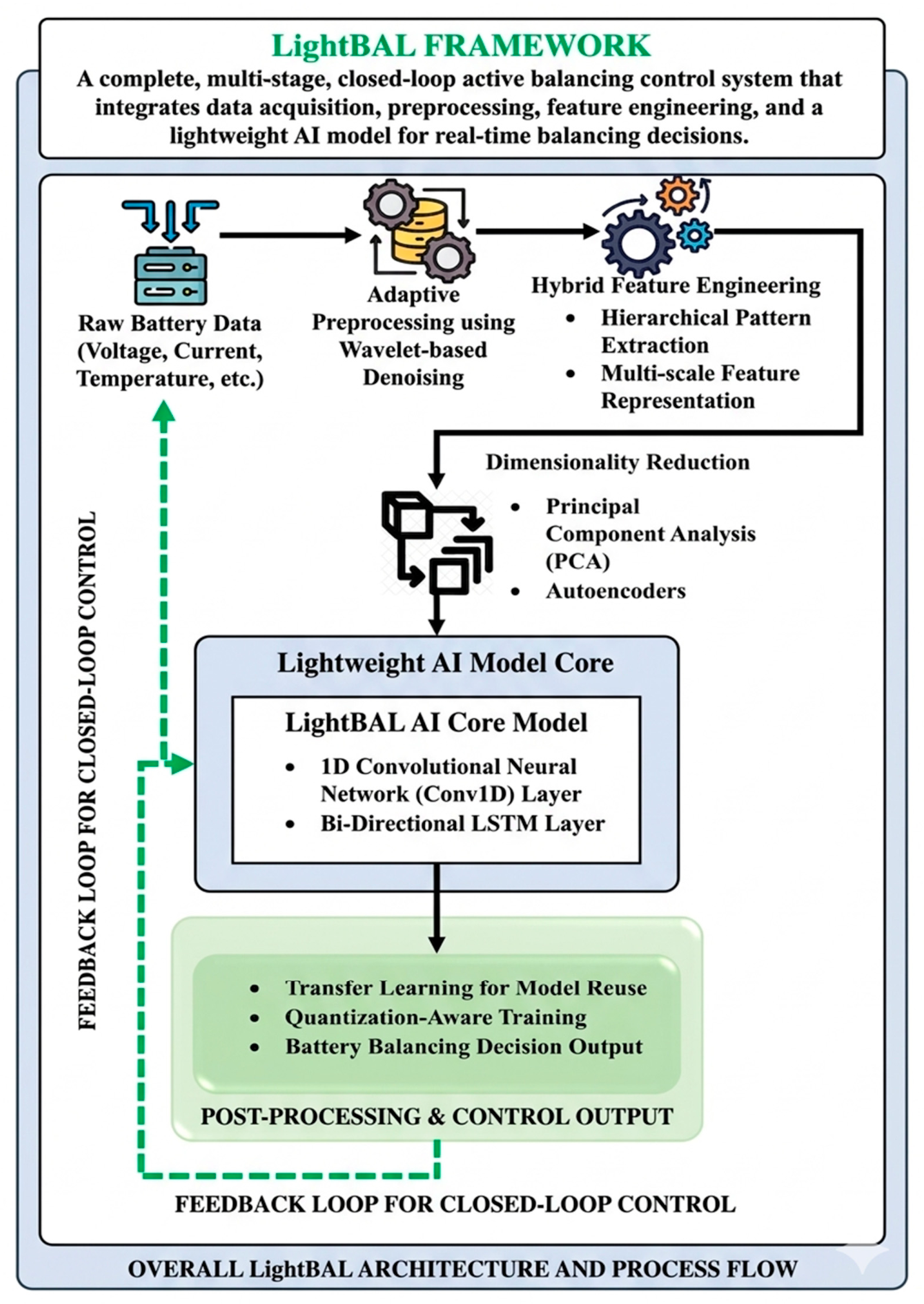
In this study, we propose a lightweight AI-based active cell-balancing approach, LightBAL, for the resource-constrained EV BMS. The proposed system employs a closed-loop sequential pipeline consisting of a preprocessing step for multivariate battery signals and hierarchical feature engineering along with PCA and autoencoder-based dimension reduction. Subsequently, the extracted and reduced features are forwarded into a lightweight Conv1D-BiLSTM prediction model through quantisation-aware transfer learning to predict the cell-level indicators, including cell voltage deviation and cell SoC drift. Finally, the predicted indicators are applied to the proportional controller to perform real-time cell balancing with acceptable results and low complexity.

Figure 1 above demonstrates the overall control system, which consists of multi-stage, closed-loop active balancing based on raw data acquisition from batteries, adaptive preprocessing, hybrid feature engineering, dimension reduction, the lightweight AI core model, and, finally, real-time postprocessing of active-balancing decisions.

3.1. Dataset Description and Experimental Conditions

This dataset contains nearly 10,000 multivariate time-series samples created through a physics-informed simulation of a 6-cell lithium-ion battery pack built in a 6S1P setup. The simulation used to create the dataset was run a few times, under various charging/discharging/idle profiles that resemble those experienced by an EV, offering diversity to benchmark the presented LightBAL framework properly.

• Parameters at pack-level (e.g., voltage, current, temperature, charging/discharging status).
• The parameters for individual cells (e.g., voltage, temperature, SoC, balancing status, and current for all 6 cells).

The dataset was created from the simulation of a physics-informed first-order Rint equivalent circuit model with thermal dynamics and an active-balancing mechanism. This dataset was developed based on a wide range of operating conditions covering a full spectrum of charge/discharge rates (0–3 C), ambient temperatures (15–60 °C), and initial state of charge (SoC) (10–90%). To emulate the cell-to-cell variation commonly observed in batteries, we added Gaussian noise to the SoC and internal resistance of the cells to simulate imbalance conditions.

The simulation framework can capture the short-term electrical and thermal behaviour of the battery cells; however, it cannot model long-term ageing mechanisms such as the growth of SEI, lithium plating, or capacity fade. The generated dataset was partitioned into chronological training (70%), validation (15%) and test (15%) datasets. For statistical reliability, the presented performance metrics were averaged over multiple runs.

Methodology for Scalability Evaluation

We first trained the LightBAL model on the dataset of a 6S1P (six-series, one-parallel) lithium-ion battery pack. In practice, it is time-consuming and costly to obtain battery data with hundreds of cells. As such, we performed a scalability study by artificially extending our validated 6S1P simulation platform to larger virtual battery packs.

Specifically, we generated 24S1P, 50S1P, 100S1P and 200S1P virtual battery packs by adding corresponding virtual cell instances on top of the existing ones, keeping the electrical and thermal properties, as well as balancing settings, the same as our original dataset.

Then, the cells were initialised under different initial SoC and internal resistances with diverse operation conditions to create sufficient cell-to-cell variations. Therefore, in this scalability study, we did not consider repeated trajectories, but utilised a diverse set of interacting virtual cells generated from the same physics-informed battery model.

The trained LightBAL model was applied directly to these larger battery configurations without any re-training or fine-tuning. To assess scalability, cell-level inference was conducted to predict the imbalance indicators for all the battery cells in each pack, and we measured the corresponding computational costs such as inference latency, memory usage, CPU usage and the effectiveness of balancing in terms of percentage of cells balancing in range. Hence, the reported scalability results evaluate the computational efficiency of our proposed method, not performance on actual large-scale battery datasets.

In this study, as shown in

Table 2. Dataset description and simulation configuration for the proposed model.

Component	Description
Data type	Simulation-generated time-series dataset
Battery configuration	6-cell pack
Input variables	Voltage, current, temperature, SoC, balancing status
Output variables	Balancing current, imbalance indicators
Operating modes	Charge, discharge, rest
Temperature	Ambient + simulated thermal dynamics
Chemistry	Lithium-ion (representative, model-based)
Aging	Not explicitly modelled
Samples	~10,000
Train/val/test split	70%/15%/15%
Validation	Multiple runs (averaged results)

, a first-order Rint equivalent circuit models each cell, and its internal resistance depends on time. Battery cells are assumed to operate under the same uniform ambient temperature, with no thermal interaction between adjacent cells. Cell capacity is assumed constant in each simulation cycle.

An active-balancing circuit controls the balancing current, transferring current between cells. The controlled active cell balancing is implemented using an active-balancing circuit.

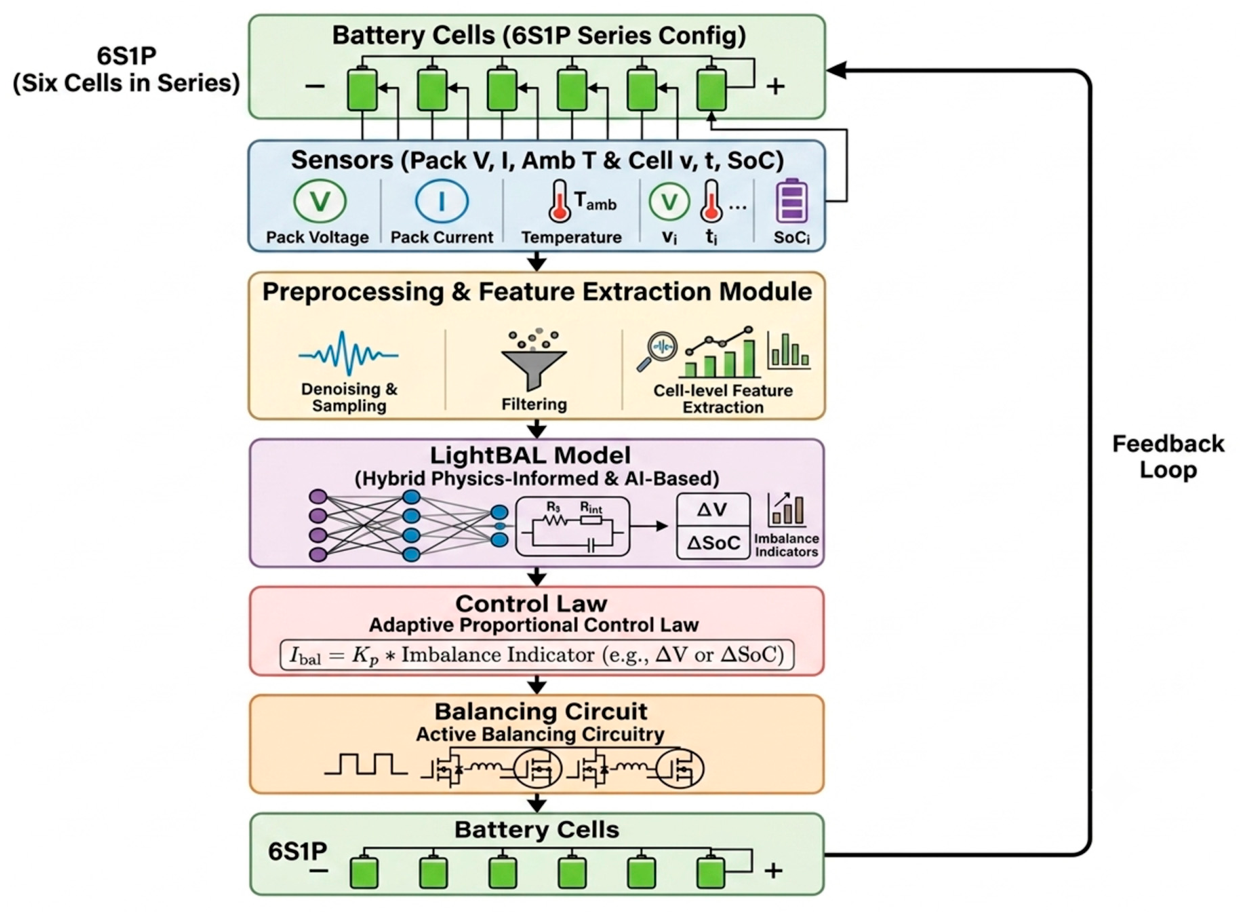
As illustrated in Figure 2, instead of computing instantaneous cell voltage offset and/or SoC offset directly from instantaneous battery current measurements, the LightBAL model discovers the nonlinear spatial–temporal interdependencies between cell voltage, current, temperature, SoC, and internal resistance from the multivariate time series of past measurements.

Instead of computing instantaneous cell voltage offset and/or SoC offset directly from instantaneous battery current measurements, the LightBAL model discovers the non-linear spatial–temporal interdependencies between cell voltage, current, temperature, SoC, and internal resistance from the multivariate time series of past measurements. Leveraging these discovered temporal dynamics, the LightBAL model predicts the future imbalance indicators (i.e., cell voltage drift and SoC drift) in the coming control interval (i.e., one-step ahead prediction).

Therefore, the balancing controller can issue appropriate proactive control actions based on the predicted future imbalance, instead of reactive actions based on instantaneous measurements.

As a result, the developed framework can represent dynamic imbalance behaviour originating from various charging/discharging rates, temperature transients, and cell interdependencies that rule-based control algorithms cannot adequately characterise. Predicted future imbalance indicators can then be translated into balancing control commands using physics-informed proportional control laws, resulting in a data-driven, predictive, and physics-based closed-loop control structure suitable for real-time BMS embedded applications.

During each simulation, cell capacity remains unchanged. Active-balancing circuitry adjusts the current transmitted between cells to implement controlled active cell balancing.

3.2. Technical Justification of Innovation

Today: Much of the current research on smart BMS concentrates on better topologies of the BMS or on the design and operation of active and passive balancing networks, and very little effort has been made on feature hierarchical engineering and the real-time constraint for the embedded implementation. Most lightweight SoC estimation approaches focus on inference efficiency and have not considered closed-loop active balancing or the dynamic relationship between balancing decisions and changing battery conditions. In addition, most present methods adopt simple preprocessing (like moving averages or traditional filters), which may not be competent to cope with transient noise from EVs’ drive conditions. Intelligent model optimisations like knowledge distillation and quantisation-aware training (QAT) have also received scant consideration in terms of implementation on microcontroller-based BMSs.

3.3. Physics-Informed Battery System Modelling

An EV battery pack is simulated using physics-informed models that emulate electrochemical behaviour, including cell voltage $V_i(t)$, current $I_i(t)$, temperature $T_i(t)$, state of charge $So{C}_i(t)$, internal resistance $R_i(t)$, and balancing current $I_{bal,i}(t)$.state of charge $So{C}_i(t)$, internal resistance $R_i(t)$, and balancing current $I_{bal,i}(t)$. A hybrid physics-based battery model and AI-driven balancing controller approach is applied, by which the Rint equivalent-circuit model estimates the terminal voltage at each sampling instant while SoC and thermal dynamics update the battery states. The cell imbalance indicators, including cell voltage deviation and cell state-of-charge (SoC) drift of every cell, are calculated using the LightBAL neural network; These predicted indicators are then provided to a proportional controller, which calculates the cell-level balancing current, $I_{bal,i}$, and feeds it into the active-balancing circuit.

3.3.1. Electrical Subsystem: Rint Equivalent Circuit Model

The electrical behaviour of each cell is represented using the classical Rint equivalent circuit model, where the terminal voltage is defined as the difference between the open-circuit voltage and the internal resistive drop. This relationship is expressed as:

$$V_i(t)=OCV(So{C}_i(t))-R_i(t) I_i(t)$$

(1)

In this formulation, $I_i(t)$ denotes the total cell current. Under normal operation without balancing action, the total current equals the load current, i.e., $I_i(t)=I_{load}(t)$.

In practical operation, the total cell current comprises both the load current and the balancing current introduced by the active-balancing mechanism $I_i(t)=I_{\mathrm{load}}(t)$. In practical operation, the total cell current consists of both the load current and the balancing current introduced by the active-balancing mechanism:

$$I_i(t)=I_{\mathrm{load}}(t)+I_{\mathrm{bal},i}(t)$$

Accordingly, the terminal voltage is more accurately described as:

$$V_i(t)=OCV(So{C}_i(t))-R_i(t)(I_{load}(t)+I_{bal,i}(t))$$

(2)

This formulation explicitly captures the influence of balancing actions on terminal voltage behaviour through additional resistive voltage drops, thereby enabling a more realistic representation of intra-pack interactions.

3.3.2. State of Charge Dynamics

The state of charge (SoC) of each cell evolves according to the net current flow, representing the energy depletion or replenishment process over time. For a discrete-time formulation with sampling interval $\mathsf{\Delta }t$, the SoC dynamics are given by:

$$So{C}_i(t+\mathsf{\Delta }t)=So{C}_i(t)-{\displaystyle \frac{I_i(t) \mathsf{\Delta }t}{C_i}}$$

(3)

where $C_i$ denotes the nominal capacity of the cell $i$. This formulation ensures consistent tracking of charge variation across charging and discharging cycles while preserving energy conservation principles.

3.3.3. Thermal Subsystem Model

The thermal dynamics of each cell are modelled using a lumped-parameter heat transfer representation that accounts for resistive heat generation and convective heat dissipation. The temperature evolution is governed by:

$${\displaystyle \frac{d{T}_i(t)}{dt}}={\displaystyle \frac{I_i^2(t) R_i(t)}{C_{th}}}-{\displaystyle \frac{T_i(t)-T_{amb}}{R_{th}{C}_{th}}}$$

(4)

where $C_{th}$ is the thermal capacity, $R_{th}$ is the thermal resistance, and $T_{amb}$ denotes the ambient temperature. The first term represents Joule heating due to internal resistance, while the second term models heat dissipation to the environment.

3.3.4. Active-Balancing Control Logic

Active cell balancing is implemented to mitigate voltage and charge imbalance across the battery pack. The balancing current is regulated based on the deviation of each cell voltage from the pack-average voltage. $\overline{V}(t)$. The control law is defined as:

$$I_{bal,i}(t)=\{\begin{array}{cc}\alpha (V_i(t)-\overline{V}(t)),& \mathrm{if} V_i(t)>\overline{V}(t)+ϵ\\ 0,& \mathrm{otherwise}\end{array}$$

(5)

where $\alpha$ is a proportional gain and $ϵ$ is a predefined tolerance threshold to prevent unnecessary switching under minor voltage variations. This strategy ensures voltage equalisation across cells, improves pack uniformity, and enhances operational reliability.

In the proposed framework, the balancing current $I_{bal}$ is not directly generated by the neural network but is computed through a defined control law based on voltage deviation, utilising the estimated imbalance states provided by LightBAL to separate AI-based state estimation from physical control implementation. Physically, active balancing is assumed to be implemented using a bidirectional DC–DC converter-based energy transfer topology, where excess energy from higher-voltage cells is redistributed to lower-voltage cells through a controlled switching network. In this energy transfer process, the source cell is chosen as the one with the greatest voltage deviation above the average pack voltage. The receiver cell is chosen as the one with the smallest voltage or the largest negative SoC deviation. The converter controller decides the energy direction from the two cells by comparing voltages. In other words, it is not a process of extracting energy from the overvoltage cell but transferring available energy from the source cell to the receiver cell. The balancing current is realised through duty-cycle modulation of the converter switches—subject to a maximum current limit to ensure safe operation—where the AI-generated control decisions are mapped to the converter switching signals to regulate both the magnitude and direction of $I_{bal}$, establishing a closed-loop, AI-assisted active-balancing framework directly governed by the learned control policy.

As shown in

Table 3. Nomenclature and symbol definitions for battery system model.

Symbol	Description	Unit
($V_i$)	Terminal voltage of cell i	V
(OCV)	Open-circuit voltage	V
($I_i$)	Cell current	A
$I_{load}$	Load current	A
$I_{bal,i}$	Balancing current	A
$R_i$	Internal resistance	Ω
$So{C}_i$	State of charge	%
$T_i$	Cell temperature	°C or K
$T_{amp}$	Ambient temperature	°C or K
$C_i$	Cell capacity	Ah
$C_{th}$	Thermal capacity	J/K
$R_{th}$	Thermal resistance	K/W
α	Balancing proportional gain	A/V
ϵ	Voltage imbalance threshold	V

, the model defines all key electrical, thermal, and balancing-related symbols along with their corresponding units used in the battery system formulation.

The underlying physical model represents each battery cell as a first-order Rint equivalent circuit with a time-varying internal resistance and assumes homogeneous ambient temperature and negligible heat conduction between neighbouring cells. Cell capacities are considered constant within one operational cycle, whereas instantaneous balancing current is injected through the active-balancing circuit to achieve pack balancing. These assumptions help to simplify the model while retaining sufficient thermal and electrical dynamics to enable real-time cell balancing.

3.4. Dataset Preprocessing and Filtering

The dataset follows a consistent preprocessing pipeline that emphasises signal quality and standardisation to enable robust feature extraction while retaining the unique physical characteristics of cell voltage, current, temperature, SoC, and internal resistance. We used wavelet-based denoising, paired with dynamic sampling, for the voltage and current signals to mitigate high-frequency noise associated with changes in electrical load or cell-balancing actions. Adaptive low-pass filtering with gradient-based feature extraction is applied to the temperature sensor data to remove the high-frequency noise while highlighting genuine thermal drift patterns. Moving-window regression is used on the collected voltage–current pairs for real-time internal resistance estimation. Each state variable is processed individually based on its respective physical behaviour to preserve the essential electrochemical and thermal information required for model learning.

The experimental dataset also captures the impact of active-balancing operation on the measured state information and the set of control inputs. Hence, the balancing current $I_{bal}$, corresponding to the DC–DC energy-balancing system, is calculated in the simulation using the active-balancing control law. This enables the generated dataset to capture the closed-loop interactions between the battery states and balancing actions. $I_{bal}$ is thus utilised to construct those closed-loop interactions between the system components and is never employed as an input for model training, i.e., the ML process only depends on non-controlled state variables such as voltages, currents, temperature, SoC, and resistance, and so on.

3.5. Signal Preprocessing and Noise Mitigation

3.5.1. Wavelet-Based Denoising

Raw sensor measurements are typically affected by high-frequency noise arising from switching events, electromagnetic interference, and sensor-level limitations. To mitigate these effects, discrete wavelet transform (DWT) is applied to both voltage and current signals.

The wavelet coefficients are decomposed, and only the significant coefficients are retained. $W_j(t)$ is retained while suppressing noise-dominant components. The reconstructed denoised signal is expressed as:

$$\tilde{X}(t)={\displaystyle \sum _{j=1}^N}{W}_j(t)$$

(6)

The above procedure eliminates high-frequency noise from the signal while retaining the critical dynamics.

3.5.2. Anomaly Detection and Missing Data Interpolation

We introduce an autoencoder (AE)-based system to deal with irregular sensor signals such as outages, spikes, and data loss. Training the AE involves learning normal operating states for all cells and detecting anomalies when reconstruction loss is significant relative to the original measurements. Anomalies are filtered out of the data or appropriately interpolated to maintain data completeness.

• Anomaly Detection: Large reconstruction loss compared to the input indicates abnormal sensor signals. The AE is trained on the normal behaviour data, so deviations from expected patterns will trigger high loss.
• Missing Data Reconstruction: If missing data are encountered, they can be effectively filled using the trained AE that considers dependencies between different cell state variables (voltage, current, temperature, and SoC).

This dual functionality enhances data integrity and ensures robustness in subsequent modelling stages.

3.5.3. Dynamic Sampling and State-Driven Filtering

To achieve computational efficiency and lower communication overhead, an event-driven adaptive sampling scheme is utilised during the dataset generation process. Instead of using a uniform sampling rate, the sampling rate of data acquisition changes based on the operating condition of the battery and on the amount of variation in cell temperature and voltage. As there are three main modes of battery operation, namely idle, charging, and discharging, each mode exhibits distinct electrical and thermal behaviour.these different modes of operation would have a unique set of electrical and thermal behaviours. This varying behaviour necessitates event-based adaptive sampling technique to accurately observe transient behaviour when transitioning between states while reducing measurements when not experiencing rapidly varying behaviour.

Then the variation in cell voltage and temperature between two successive instants of samples is expressed as follows.

Change detection is defined as:

$$\mathsf{\Delta }{V}_i(t)=\mid V_i(t)-V_i(t-\mathsf{\Delta }t)\mid$$

(7)

$$\mathsf{\Delta }{T}_i(t)=\mid T_i(t)-T_i(t-\mathsf{\Delta }t)\mid$$

(8)

where $V_i\left(t\right)$ and $T_i\left(t\right)$ denote the voltage and temperature of the $i^{th}$ cell at time t, respectively.

A threshold-based triggering condition is defined as:

$$\mathsf{\Delta }{V}_i(t)>{\delta }_V\mathrm{or}\mathsf{\Delta }{T}_i(t)>{\delta }_T$$

(9)

where ${\delta }_v$ and ${\delta }_T$ represent the voltage and temperature thresholds.

The adaptive sampling frequency is given by:

$$S_i(t)=\{\begin{array}{cc}{f}_{high},& \mathrm{if} \mathsf{\Delta }{V}_i(t)>{\delta }_V \mathrm{or} \mathsf{\Delta }{T}_i(t)>{\delta }_T\\ f_{low},& \mathrm{otherwise}\end{array}$$

(10)

A state-dependent weighting function is further defined as:

$$w_i(t)={\gamma }_1\mathsf{\Delta }{V}_i(t)+{\gamma }_2\mathsf{\Delta }{T}_i(t)$$

(11)

where ${\gamma }_1$ and ${\gamma }_2$ are weighting coefficients that determine the relative importance of voltage and temperature variations.

Using this activity measure, the sampling interval is adaptively adjusted according to

$$\mathsf{\Delta }{t}_i(t)=\mathsf{\Delta }{t}_{min}+{\displaystyle \frac{1}{1+w_i(t)}}(\mathsf{\Delta }{t}_{max}-\mathsf{\Delta }{t}_{min})$$

(12)

where $\mathsf{\Delta }{t}_{\min }$ and $\mathsf{\Delta }{t}_{\max }$ denote the minimum and maximum allowable sampling intervals, respectively. Larger state variations result in shorter sampling intervals, whereas stable conditions permit longer intervals.

To prevent frequent switching between high- and low-frequency sampling, a memory term is incorporated:

$$M_i(t)=\{\begin{array}{cc}1,& \mathrm{if} \mathrm{threshold} \mathrm{condition} \mathrm{is} \mathrm{satisfied}\\ \mathrm{m}\mathrm{a}\mathrm{x}(0,M_i(t-\mathsf{\Delta }t)-\lambda \mathsf{\Delta }t),& \mathrm{otherwise}\end{array}$$

(13)

where the decay rate controls the decrease in memory with time.

Lastly, the effective sample rate is governed by

$$S_i(t)=f_{low}+M_i(t)(f_{high}-f_{low})$$

(14)

which enables a smooth transition between low- and high-frequency sampling while maintaining responsiveness to transient battery dynamics and avoiding unnecessary oscillations in the sampling process.

3.6. Feature Engineering and Dimensionality Reduction

The hierarchical features are generated from the raw measurements of voltage, current, temperature and SoC to better represent the behaviour of the battery, such as cell imbalance, thermal behaviour, ageing, and battery dynamics. Voltage Imbalance: The divergence of individual cell voltages from the pack-averaged voltage is calculated by

$$\mathsf{\Delta }{V}_i=V_i-\overline{V},\overline{V}={\displaystyle \frac{1}{N}}{\displaystyle \sum _{i=1}^N}{V}_i$$

(15)

This feature captures cell-level deviation from pack average voltage and is critical for imbalance detection.

Temperature Gradient: Thermal variations are specified by either the space gradient or the time gradient of temperature.

$$\nabla T_i={\displaystyle \frac{d{T}_i}{dx}} \mathrm{or} {\displaystyle \frac{d{T}_i}{dt}}$$

(16)

where $T_i$ is the temperature of the $i^{th}$ cell. This feature detects abnormal internal temperatures with a non-uniform distribution or rapid changes, which indicate abnormalities in the operation of the cell.

The internal resistance of a cell is estimated to

$$R_i={\displaystyle \frac{V_i}{I_i}}$$

(17)

where i is the cell current; cell degradation or ageing normally causes higher internal resistance.

Additionally, other dynamic characteristics, including voltage recovery speed, rate of change in SoC, and entropy-based indicators of stability, are extracted to characterise the battery pack’s dynamic behaviour.

3.6.1. Dimensionality Reduction

The handcrafted feature vector extracted previously may include correlated or redundant features. Therefore, the dimensionality of the feature set is reduced for higher computational efficiency.

Principal Component Analysis (PCA):

$$Z=X\cdot W$$

(18)

such that X is the feature matrix, W contains the principal component vectors, and Z is the compressed representation for the features by projecting them into the principal component space.

Aut

$$h=f_{encoder}(x),\widehat{x}=f_{decoder}(h)$$

(19)

where x is the input feature vector, h is the low-dimensional latent representation generated by the encoder, and $\hat{x}$ is the reconstructed output. The latent vector h is used as the compact feature representation for subsequent model training.

3.6.2. Feature Selection Using Information Gain

We use the feature selection criterion information gain (IG) to filter the most descriptive attributes from:

$$IG(Y,X)=H(Y)-H(Y\mid X)$$

(20)

where $H(Y)$ denotes the entropy of the target variable and $H(Y\mid X)$ represents the conditional entropy after observing feature $X$. Features with higher information gain provide greater predictive value and are retained for training. Features with higher information gain provide greater predictive value and are retained for training. In contrast, less informative features are discarded to reduce redundancy and computational complexity.

3.6.3. Closed-Loop Active Cell-Balancing Scheme

The LightBAL framework achieves active cell balancing through a bidirectional DC-DC converter which operates under a closed-loop control strategy. The higher-voltage cell(s) charge the lower-voltage cell(s) by modifying the switches’ duty cycle. At the same time, the cell-balancing current remains within a set security margin. Instead of directly managing the power converter, the LightBAL neural network acts as an imbalance estimator which receives the preprocessed battery state vector and predicts cell voltage deviation and cell SoC drift. These imbalances are translated to a balancing current command via a proportional controller. Based on the desired current, the converter duty cycle is determined, thereby controlling the direction of energy transfer between cells. During the following time interval, the updated balancing current is fed into the battery model, establishing a closed loop which uses an AI-based imbalance estimate within a physics-informed active cell-balancing control strategy.

3.7. LightBAL Framework Design

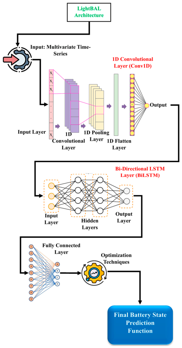
A lightweight, efficient deep learning architecture is proposed in Figure 3 to make accurate predictions of battery cell states for forecasting and balancing decisions, and it is deployed in real time on a low-power BMS hardware platform. Figure 3 shows the proposed architecture of the LightBAL design.

3.7.1. LightBAL Base Model Design

Our proposed LightBAL framework uses a lightweight Conv1D-BiLSTM model that enables it to simultaneously capture spatial correlations between different battery variables and the time dependence throughout battery operation. We provide multivariate time-series data (e.g., cell voltage, current, temperature, state of charge (SoC), internal resistance) as input for our model, which is suitable for embedding on a small device.

3.7.2. Conv1D Layer

Given the multivariate input sequence of the $i^{th}$ battery cell,

$$X_i =[x_i^1 ,x_i^2 ,\dots ,x_i^T ]\in R^{T\times F}$$

(21)

where $T$ is the sequence length, and $F$ denotes the number of input features. The Conv1D layer extracts local temporal patterns using

$$z_t^k=\sigma \left({\displaystyle \sum _{j=0}^{\omega -1}{\displaystyle \sum _{f=1}^F{W}_j^k,f^{x_{t+j,f}+b^k}}}\right)$$

(22)

where $W^k$ and $b^k$ are the weights and bias of the $k^{th}$ convolution kernel, w is the kernel size, and $\sigma \left(\right)$ stands for the activation function. Convolution generates a feature map containing information about the short-term dynamics of the battery and attenuating measurement noise.

3.7.3. BiLSTM Layer

After being extracted through convolutional features, we process the values with a Bidirectional Long Short-Term Memory (BiLSTM) network to capture long-term temporal dependencies. The forward and backwards hidden states are calculated as:

$${\overrightarrow{h}}_t=LST{M}_{fwd}\left(z_t,{\overrightarrow{h}}_{t-1}\right),{\overleftarrow{h}}_t=LST{M}_{fwd}\left(z_t,{\overleftarrow{h}}_{t-1}\right)$$

(23)

The concatenated BiLSTM output:

$$H_t=\left[{\overrightarrow{h}}_t;{\overleftarrow{h}}_t\right]$$

(24)

where $H_t$ represents the fused temporal feature vector at time t.

The overall feature extraction process is therefore expressed as

$$H=BiLSTM\left(Conv1D\left(X\right)\right)$$

(25)

where $H$ is the learned spatio-temporal representation used for subsequent prediction.

3.7.4. Model Optimisation

We present 3 lightweight optimisations that allow our model to be readily deployed in an embedded battery management system (BMS). Knowledge Distillation: We train a smaller student model to mimic knowledge distilled from the larger teacher network. The optimisation objective function of (a) can be interpreted as

$$L_{KD }=\lambda KL(P_T \mid \mid P_S )+(1-\lambda )L_{CE}$$

(26)

where $P_T$ and $P_S$ are the teacher and student probability distributions, KL(⋅) denotes the Kullback–Leibler divergence, $L_{CE}$ is the cross-entropy loss, and λ balances the two objectives.

Quantisation-Aware Training

Model parameters can be quantised during training to reduce the amount of memory and the inference latency:

$$Q_{quant}=Quantize\left({\theta }_{float}\right)$$

(27)

Floating-point parameters can be mapped to low-precision numbers without loss of prediction accuracy.

Layer Freezing

The early convolutional layers were then frozen in during fine-tuning when training completed:

$${\displaystyle \frac{\partial L}{\partial {\theta }_{frozen}}}=0$$

(28)

This will allow us to simplify our training by not having to re-train the static feature extractors.

3.7.5. The Prediction Model

After optimisation, the lightweight model predicts battery imbalance indicators based on the input sequence:

$$\widehat{Y_i}=LightBALL\left(X_i;{\theta }_{light}\right)$$

(29)

where $x_i$ is the input sequence of the $i$th cell, ${\theta }_{\mathrm{L}\mathrm{i}\mathrm{g}\mathrm{h}\mathrm{t}\mathrm{B}\mathrm{A}\mathrm{L}}$ represents the optimised model parameters, and $y_i$ represents the cell-deviation indicators, including voltage drop and SoC drift.

3.7.6. Prediction Task Design and Training Objective

To obtain more continuous states related to battery imbalance (such as future states tending to be unbalanced) as prediction results, rather than a discrete state, LightBAL is designed as a multi-output regression task instead of a classification task. The input vector of the neural network includes four states of the cell voltage, current, temperature, and SOC, as well as its internal resistance after processing. Based on these temporal cell states, LightBAL predicts two future states which indicate the future imbalance trend of cells: the cell-level voltage deviation and cell-level SoC drift.

$${\hat{Y}}_i(t)=f_{\theta }(X_i(t))$$

(30)

In which $X_i\left(t\right)$ indicates the processed input sequence of the $i^{th}$ cell, $f_{\theta }$ denotes the trained Conv1D-BiLSTM model, and ${\hat{Y}}_i\left(t\right)$ shows the estimated imbalanced state:

$${\hat{Y}}_i(t)=[\mathsf{\Delta }\widehat{V_i}(t),\mathsf{\Delta }\widehat{SoC}i(t)]$$

(31)

where $\mathsf{\Delta }\widehat{V_i}(t)$ is the predicted voltage deviation and $\mathsf{\Delta }\widehat{SoC}i(t)$ is the predicted SoC drift.

Instead, we pass the unbalanced states in Equation (4) to the proportional controller in Equation (5) and calculate the balancing current, $I_{bal,i}$, according to the estimated unbalance magnitude. It allows LightBAL to run AI state estimation and provide a physical balancing control law.

We use a regression loss for the training because the targets for prediction are continuous variables. The main loss function used is mean squared error (MSE):

$$L_{MSE}={\displaystyle \frac{1}{N}}{{\displaystyle \sum _{i=1}^N\left(Y_i-\widehat{Y_i}\right)}}^2$$

(32)

where $Y_i$ and ${\hat{Y}}_i$ are the real and predicted imbalance status, respectively. We define the objective function used in training, where the entire training loss is contributed by both accuracy and knowledge transfer from the teacher.

While optimising a model, the total training loss is composed of prediction error along with the loss coming from transfer of knowledge from the teacher network:

$$L_{total }=L_{MSE} +\lambda L_{KD}$$

(33)

where $L_{KD}$ is the knowledge distillation loss from Equation (26) and $\lambda$ controls how much weight the distillation objective is given.

LightBAL therefore applies continuous imbalance state regression, so that no discrete imbalance classes are created during dataset creation. As such, the reported regression metric of MAE represents the accuracy of the predicted voltage deviations and SoC drifts directly. If classification-based metrics such as accuracy and F1-score are presented, they should strictly be regarded as supporting figures for continuous imbalance prediction across several predefined classes, and removed otherwise.

3.8. Active Cell-Balancing Simulation

The calculated voltage difference and SOC deviation are then applied to the proportional controller, which calculates the balancing current. This calculated balancing current is supplied through the bidirectional DC-DC converter and also sent back to the battery model to be used during the next control cycle.

At each balancing cycle, the source cell loses energy (stored energy decreases by the balancing current), while the receiver cell gains energy (the converter-controlled charging current recharges it). All of these energy exchanges are considered in the coming SoC and voltage calculations.

3.8.1. Balancing Triggering

Active cell balancing works only when the highest voltage or SoC discrepancy exceeds the threshold given by (34).

$$max(\mathsf{\Delta }{V}_i )>{\delta }_{V }or max(\mathsf{\Delta }SoCi )>{\delta }_{SoC}$$

(34)

where

$$\mathsf{\Delta }{V}_i =V_{i }-\stackrel{-}{V},\mathsf{\Delta }So{C}_{i }=So{C}_{i }-\overline{SoC}.$$

(35)

Here, ${\delta }_v$ and ${\delta }_{SoC}$ denote the allowable voltage and SoC imbalance thresholds.

3.8.2. Balancing Current

When balancing is activated, the converter transfers energy from cells with higher voltage to those with lower voltage.

$$Ibal,i (t)=\left\{\begin{array}{l}\alpha (V_i (t)-\overline{V}(t)), Vi (t)>\overline{V}(t)\\ 0\hspace{1em}\hspace{1em}\hspace{1em}\hspace{1em}\hspace{1em}\hspace{1em},otherwise\end{array}\right\}$$

(36)

where $\alpha$ is the balancing gain.

The balancing current that flows on the receiver end can be calculated based on the balance relation of a bidirectional DC-DC converter. Considering converter efficiency, the power transferred from the source cell to the receiver cell is

$$V_s{I}_s{\eta }_{conv}=V_r{I}_r$$

(37)

where $V_s$ and $I_s$ are the voltage and current for the source cell; $V_r$ and $I_r$ are the voltage and charging current for the receiver cell; and conv is the converter efficiency. The efficiency factor accounts for switching and conduction losses, as well as other energy-conversion losses. As a result, the actual receiver-side balancing current can be obtained as follows:

$$I_r={\displaystyle \frac{{\eta }_{conv}{V}_s{I}_s}{V_r}}$$

(38)

The above formulation guarantees that the energy transfer between cells is physically possible and differentiates this proposed active balancing from selective cells’ discharges.

$$V^{¯}(t)={\displaystyle \frac{1}{N}}{\displaystyle \sum _{i=1}^N V_i (t)}$$

(39)

is the average pack voltage.

3.8.3. SoC Update

The cell SoC after balancing is updated as

$$So{C}_{i }(t+1)=So{C}_{i }(t)-{\displaystyle \frac{I_{bal,i} (t)\mathsf{\Delta }t}{C_i}}$$

(40)

where $C_i$ is the cell capacity and Δt is the simulation time step.

3.8.4. Voltage Update

Using the equivalent-circuit (Rint) battery model, the updated terminal voltage is

$$V_{i }(t+1)=OCV(So{C}_i (t+1))-R_i (t)I_{bal,i} (t)$$

(41)

where OCV (⋅) denotes the open-circuit voltage and Ri (t) is the internal resistance of the $i^{th}$ cell.

First, we apply wavelet filtering and an autoencoder to denoise the battery measurements, including voltage, current, temperature, state of charge (SoC), and internal resistance. Then we extract hierarchical features, reduce, select, and feed them to the LightBAL model. Model Inputs: The LightBAL neural network takes processed battery state parameters such as cell voltage, current, temperature, state of charge (SoC), and internal resistance. Prediction Objectives: The neural network forecasts the battery imbalance indicators (cell voltage deviation and SoC drift). Control Signal: The proportional controller determines the balancing current from the predicted imbalance indicators. Feedback Inputs: Updated battery voltage, current, temperature, SoC, and balancing current are measured and passed back to the LightBAL neural network for the following step. We evaluate balancing performance through simulations of charging and discharging based on voltage deviation, SoC uniformity, temperature consistency, inference latency, and computation efficiency to measure both balancing ability and embedding friendliness.

3.8.5. Balancing Efficiency Definitions

For clarity of definition and understanding the distinct physical meanings of balancing, three different balancing efficiency metrics were chosen for this work, which cannot be mutually replaced and characterise distinct physical properties of the balancing process.

(1) Balancing efficiency

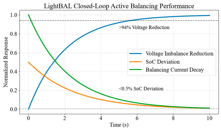
This represents the ability of the proposed LightBAL controller to mitigate cell imbalance. The balancing efficiency represents how significantly the differences in cell voltage or SoC have been reduced. It can be described in terms of voltage difference as:

$${\eta }_{bal},V ={\displaystyle \frac{\mathsf{\Delta }{V}_{initial }-\mathsf{\Delta }{V}_{final}}{\mathsf{\Delta }{V}_{initial}}} \times 100$$

(42)

where $\mathsf{\Delta }{V}_{initial }$ and $\mathsf{\Delta }{V}_{final}$ represent the maximum cell voltage difference before and after balancing, respectively.

Similarly, the SoC-based balancing efficiency is calculated as:

$${\eta }_{bal,SoC }={\displaystyle \frac{\mathsf{\Delta }So{C}_{initial }-\mathsf{\Delta }So{C}_{final} }{\mathsf{\Delta }So{C}_{initial}}} \times 100$$

(43)

where $\mathsf{\Delta }SoC$ is the maximal cell SoC difference between cells indicated as SoC.

This metric presents the reduction capability of the proposed balancing algorithm.

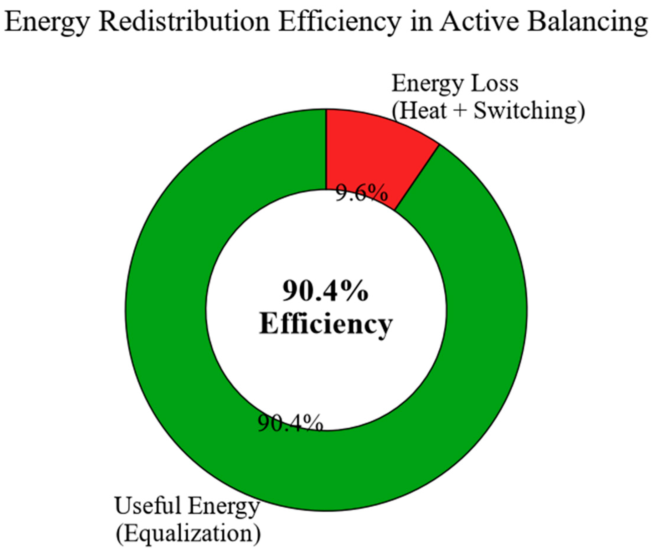
(2) Energy Redistribution Efficiency (energy)

Energy redistribution efficiency is defined as how efficiently the active-balancing circuit redistributes the energy from high-energy cells to low-energy cells.

$${\eta }_{energy} ={\displaystyle \frac{E_{received}}{E_{transferred} }}\times 100$$

(44)

where $E_{transferred}$ is the energy taken from the source cell while balancing and $E_{received}$ is the useful energy provided to the receiver cell.

This energy that is transferred will be determined by the following calculation:

$$E_{transferred }=\int V_s (t)I_{bal }(t)dt$$

(45)

And the received energy is:

$${\eta }_{eq} =1-{\displaystyle \frac{{\sigma }_{final}}{{\sigma }_{initial}}}$$

(46)

where $\sigma$ stands for the standard deviation of cell SoC (or voltage). Better cell convergence indicates a higher cell equalisation efficiency.

$$E_{received} =\int V_{r }(t)I_{bal,r }(t)dt$$

(47)

where Vs and Vr are the voltages of the source and receiver cells, respectively; this metric quantifies the energy transfer efficiency of the bidirectional dc–dc converter and incorporates converter losses.

(3) BalancingEfficiency(_eq)

The equalisation efficiency assesses the uniformity of cells in the final balanced state. Unlike the balancing efficiency, it does not measure relative imbalance to the initial state, but how equally the cells are divided in the final state.

3.9. Limitations of Simulation-Based Validation and Potential for Deployment

The LightBAL framework is validated through a computationally efficient and reproducible physics-informed simulation environment based on a Rint equivalent circuit model in combination with a simplified thermal model. This allows controlled tests across various operating conditions. Nevertheless, compared to a physical battery system, the simulation environment has certain shortcomings. First, the Rint model does not account for complex electrochemistry such as SEI growth, lithium plating, diffusion phenomena, OCV hysteresis or diffusion-induced relaxation.

In addition, the simulation assumes a relatively uniform initial state, homogeneous NMC chemistry, simple thermal dynamics without spatial temperature variation or inter-cell cooling effects, and little interaction regarding couple-ageing effects. Also, many realistic sensor issues such as measurement noise and drift, communication delay, manufacturing variations or even extreme operation conditions are not addressed.

A preliminary hardware-in-the-loop (HIL) was performed to assess the possibility of running the LightBAL model embedded on a Raspberry Pi 4. The HIL analysis mainly validates real-time capability, CPU consumption, response latency and command generation. However, the real cell-balancing currents, energy transferred, and final state-of-charge (SoC) equalisation were not physically measured, so the HIL analysis results can be interpreted as feasibility validation of embedding rather than complete battery balancing.

Future work will focus on comprehensive experimental validation using physical battery packs with different Li-ion chemistries (e.g., LFP, NMC, and LCO), real-world driving cycles (e.g., UDDS and WLTP) and extended HIL and laboratory tests under varying temperatures, ageing conditions, sensor uncertainty and operation scenarios to assess the real-world application value of the presented framework and will focus on comprehensive experimental validation using physical battery packs with different Li-ion chemistries (e.g., LFP, NMC, and LCO), real-world driving cycles (e.g., UDDS and WLTP) and extended HIL and laboratory tests under varying temperatures, ageing conditions, sensor uncertainty and operation scenarios to assess the real-world application value of the presented framework.

3.10. Practical Availability and Uncertainty of the Input Variables in a Real BMS Implementation

In the context of a real battery management system (BMS), the actual availability and accuracy of cell-level input variables could be different from those of the ideal simulation environment used in this work. While LightBAL requires cell-level state of charge (SoC), temperature, voltage, current, internal resistance, and balancing-relevant information as inputs to the model, in real battery systems these variables are commonly obtained from a combination of direct measurements and state estimation. For example, cell-level SoC is not directly measurable, and it has to be estimated using several techniques such as Coulomb Counting, Kalman Filters (KFs) and observer-based estimations. Hence, LightBAL’s predictions could be sensitive to SoC estimation errors, especially during transient states where current changes rapidly.

In the case of temperature, real BMS implementations might only measure the temperature in a subset of the cells because of cost, wiring limitations, and hardware constraints. Unmeasured cell temperature could be inferred using thermal models, spatial interpolation, and sensor fusion methods. The proposed framework could handle those estimated temperatures; nevertheless, inaccuracies due to temperature gradients, delays or unusual heating could introduce uncertainties in the prediction of imbalance.

Finally, it should be highlighted that the balancing current $I_{bal}$ is not an input required for the neural network in the proposed LightBAL architecture; it is calculated through the physical closed-loop proportional controller and the DC-DC converter control scheme. In a practical BMS, the actual balancing current can be inferred from converter operation (e.g., converter switching duty cycle, voltages across the converter, and current measured by the current sensor). The discrepancy between command and actual balancing current (e.g., due to converters’ losses, delays, etc.) can result in imperfect closed-loop balancing accuracy.

The current research does not explicitly model sensor uncertainties, estimation errors, and communication latencies. All of these issues are potential limitations that need to be addressed in future research to improve the robustness of LightBAL when applied to real-world BMS using experimental battery packs and embedded hardware. Future research will investigate the incorporation of uncertainty-aware state estimation, sensor fault tolerance techniques and adaptive learning mechanisms.

4. Results and Discussion

This Results and Discussion Section provides a detailed breakdown of the proposed LightBAL model’s performance for real-time active cell balancing in EV battery systems. The analysis evaluated multiple metrics: accuracy, latency, efficiency, and memory size. The results for the LightBAL model were compared with those of established models to demonstrate how LightBAL provides a superior solution for embedded BMS solutions.

(A) Performance Metric Definitions and Interpretation

The evaluation metrics employed in this paper are stated mathematically below, with the corresponding physical significance provided to avoid confusion and facilitate readers’ clear understanding of the results and reproducibility.

(i) Accuracy (Acc):

Accuracy denotes the ratio of correct classification decisions out of the total decisions. Accuracy is computed as:

$$Acc={\displaystyle \frac{TP+TN}{TP+TN+FP+FN}}$$

(48)

where TP, TN, FP and FN represent true positives, true negatives, false positives and false negatives, respectively. In this study, accuracy is utilised to quantify the classification of the battery state of imbalance to balance decisions, i.e., the higher the accuracy, the better the decision performance.

(ii) F1-score:

The F1-score is defined as the harmonic mean of precision and recall and is often applied as a robust metric to identify bias due to class imbalance:

$$F1={\displaystyle \frac{2\cdot (Precision\cdot Recall)}{Precision+Recall}}$$

(49)

where

$$Precision={\displaystyle \frac{TP}{TP+FP}},Recall={\displaystyle \frac{TP}{TP+FN}}$$

(50)

The framework in this paper measures the model’s capability to effectively diagnose imbalanced conditions and avoid mistakenly triggering balancing actions, i.e., to ensure balanced decision classification reliability.

(iii) Mean Absolute Error (MAE):

Mean absolute error measures the average difference magnitude between a predicted and a true continuous value:

$$MAE={\displaystyle \frac{1}{n}}{\displaystyle {\sum }_{i=1}^n}\mid y_i-{\widehat{y}}_i\mid$$

(51)

where $y_i$ is the ground truth and ${\widehat{y}}_i$ is the predicted value. In our work, MAE is implemented on the voltage deviation (V) and the SoC imbalance (%) to determine the regression accuracy. Lower MAE denotes better performance.

(iv) Memory Footprint:

Memory footprint represents the storage requirement of the LightBAL model during inference deployment, including all its parameters and the related computational overhead. It is computed as:

$$Memory(MB)={\displaystyle \frac{N_p\times b}{8\times {1024}^2}}$$

(52)

where Np is the number of parameters of the model, and b is the number of bits per parameter. This metric indicates how suitable the trained model is for embedded hardware-based BMS due to their resource constraints (e.g., memory size). Lower memory footprint represents greater hardware efficiency.

(v) Inference Latency:

Inference latency refers to the average time to perform one output prediction.

$$Latency={\displaystyle \frac{T_{total}}{N_{samples}}}$$

(53)

where $T_{total}$ is the total execution time and $N_{samples}$ is the number of inference samplesThis is important for evaluating the efficiency of the LightBAL framework for real-time balancing decisions. Lower latency enables faster and more responsive balancing control. Lower latency means faster and more appropriate.

(B) Unified Experimental Framework and Baseline Fairness

All other evaluated baseline models (ANN, LSTM, CNN, and conventional TL) were trained, preprocessed, and evaluated on the same experimental pipeline to ensure fairness in comparison.

• Data Partitioning Fairness: The entire dataset was partitioned in the same ways (70%, 15%, and 15% for training, validation, and testing splits, respectively), keeping the same order of sample timestamps.
• Preprocessing Uniformity: The same processing steps, including wavelet denoising, hierarchical features learning, and PCA-AE-based dimensionality reduction, were applied to the same inputs to train all baseline models and the LightBAL framework. This ensures that all baseline models were provided with the same input data, eliminating possible biases due to preprocessing.
• Optimisation and Hyperparameter Alignment: Standard hyperparameters are used for all baseline models reported in the relevant literature. Limited hyperparameter tuning using grid search over a reasonable range is conducted for all baselines.

However, without special optimisations like knowledge distillation, quantisation-aware training, or additional fine-tuning strategies that favour particular model architectures or learning algorithms, these baseline models are disadvantaged or evaluated more fairly.

4.1. Performance Evaluation of the LightBAL

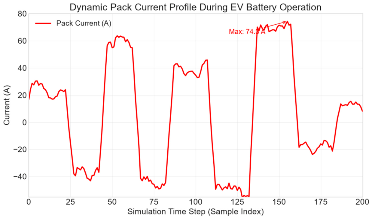
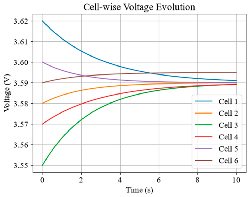
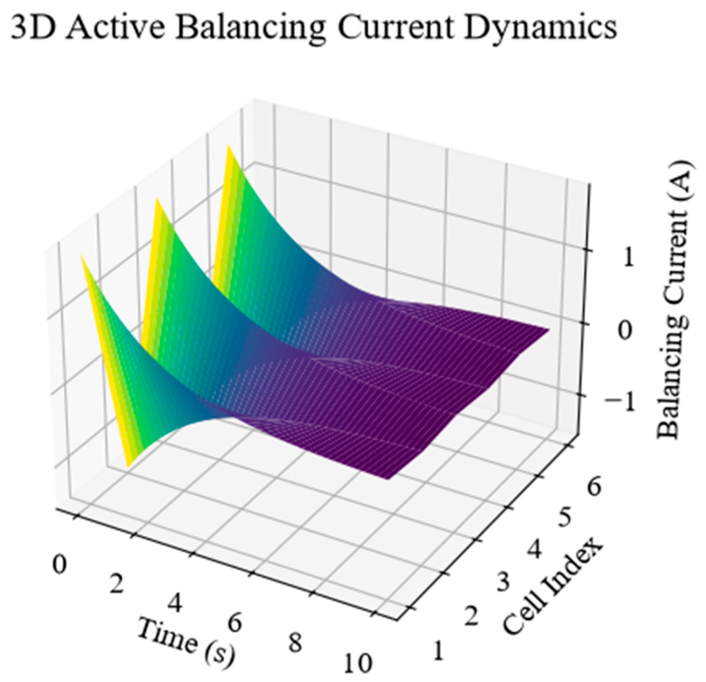
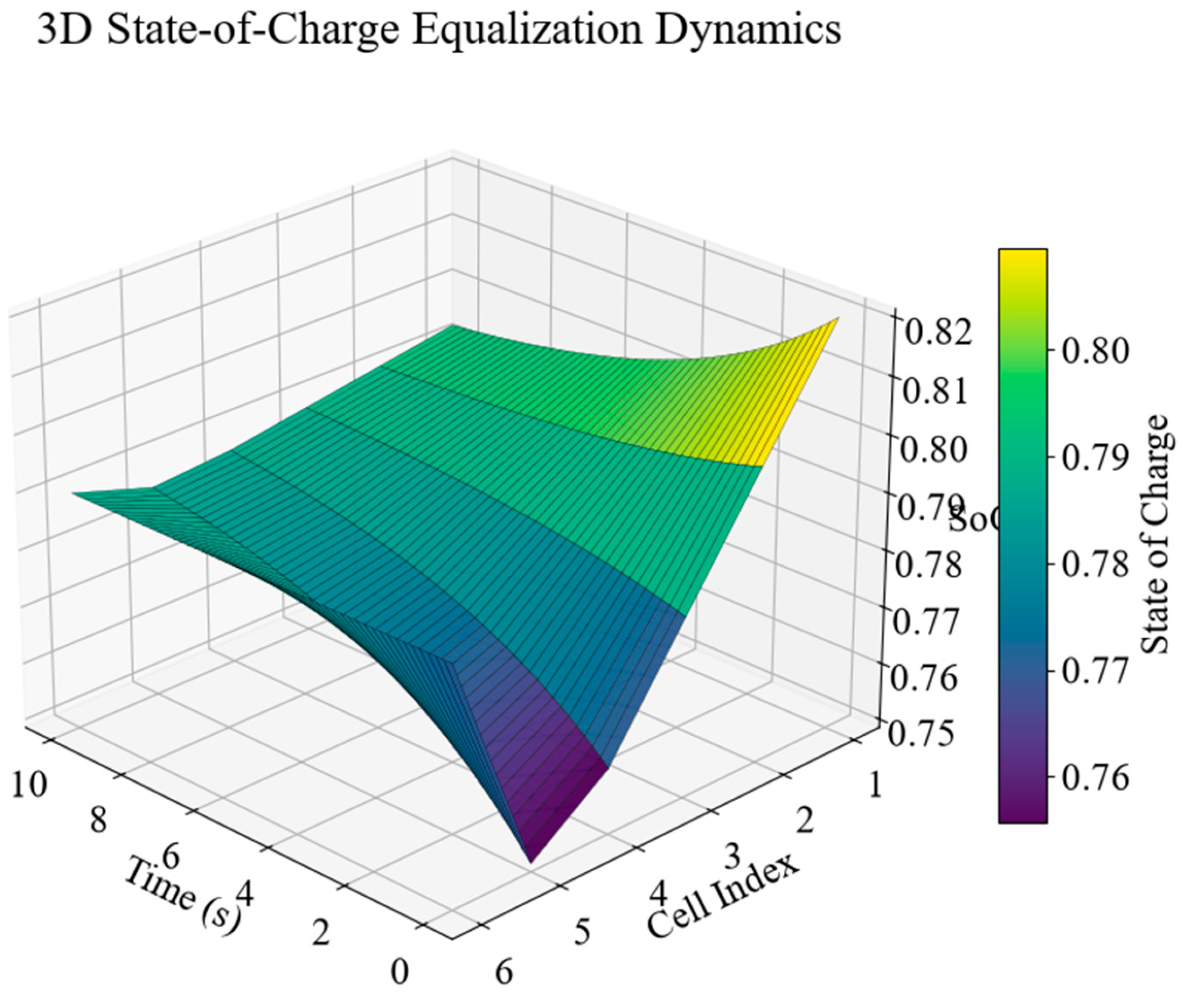
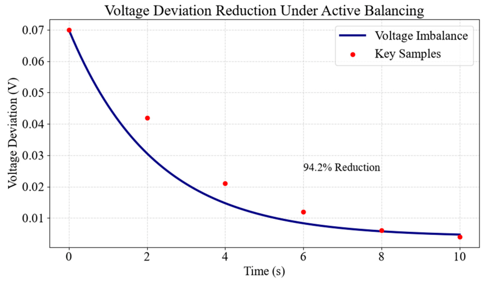
The proposed LightBAL model is assessed in a desktop simulation environment over 200 consecutive iterations to evaluate key performance metrics including SoC uniformity, thermal dynamics, voltage profiles, and current distribution under controlled EV operational scenarios. For the results presented in Figure 4, Figure 5 and Figure 6, the x-axis signifies the sequential simulation iteration (sample index), not a fixed physical time duration. Therefore, these plots demonstrate the behaviour and response characteristics of the models over multiple battery states across 200 iterations; no consistent sampling frequency or total duration in seconds is applicable.

The simulation framework offers controlled evaluation settings, but it does not capture all potential battery uncertainties in a real-life scenario such as ageing degradation, imperfect sensors, manufactory variations, or chemical-specific electrochemistry.

Experimental Verification Methodology: An overall three-stage validation procedure was carried out to assess the proposed LightBAL framework in its entirety. Initially, offline simulations of the balancing algorithm were carried out to study the controller’s performance under stable operation. Subsequently, the optimised model was embedded into a Raspberry Pi 4 and verified using a real-time hardware-in-the-loop (HIL) experimental platform consisting of a commercial battery emulator, an embedded controller, an active-balancing circuit, and the relevant sensor interfaces. The real-time operation capability of the designed controller and closed-loop balancing performance under typical driving-cycle current profiles were further verified via HIL experiments. Thus, both simulation and experimental HIL verification will be discussed in this paper.

Figure 4 showcases the simulated pack current profile across 200 iterations under varied EV operating states. Current fluctuates between −50 A (discharge) and +75 A (charge), representing typical scenarios like acceleration, regenerative braking, and idling. Notable shifts in load occur at time steps 25, 50, and 75, corresponding to abrupt changes in the battery pack’s power demand and energy recuperation. Despite these variations, the LightBAL model effectively redistributes current to ensure uniform charge distribution among cells, minimising overall energy imbalance and enhancing charge equalisation during dynamic loading conditions.

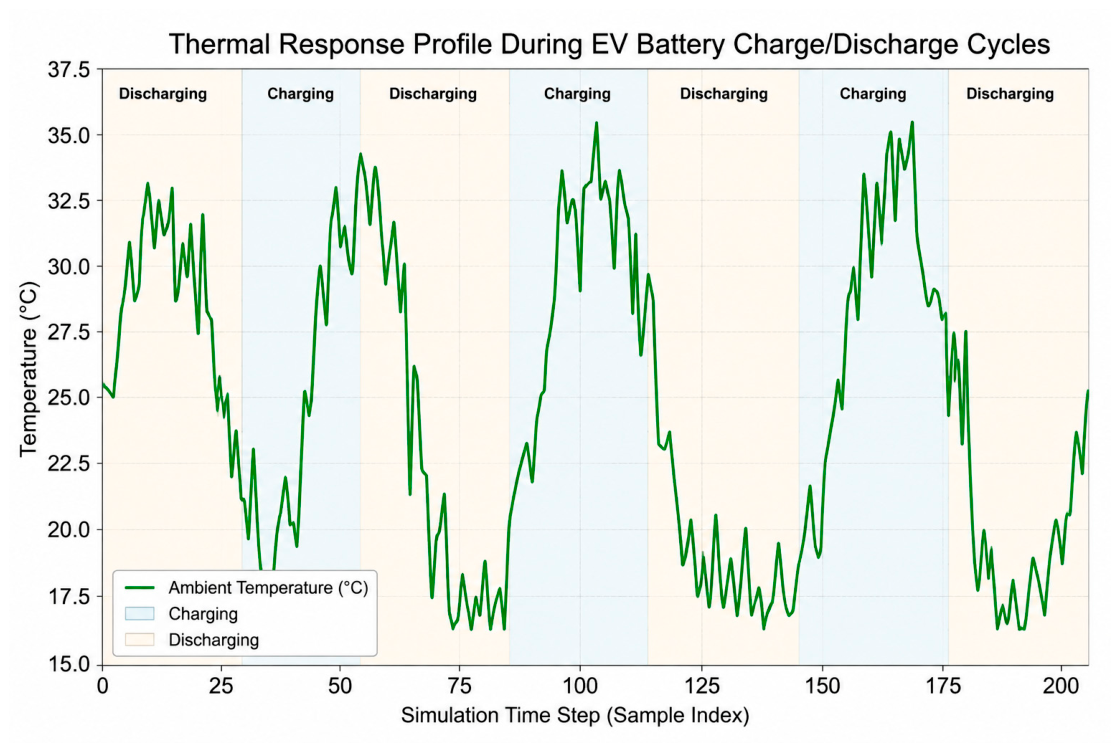
Figure 5 details the simulated thermal response across 200 iterations under extreme stress-test conditions designed solely to challenge model robustness under worst-case scenarios, even exceeding normal operating ranges for lithium-ion batteries. This simulation aims to test the model’s ability to react to rapid temperature variations and identify potential regions of thermal instability, rather than replicate normal battery behaviour. By employing these simulated thermal patterns, the framework facilitates adaptive balancing strategies that bolster thermal stability, curb the risk of overheating, and enhance battery safety.

Following scalability results (Figure 5), which do not involve an analysis of the power lost as was performed, for instance, in Section 4.9, but are measured from an HIL real-time run on real-time embedded hardware.

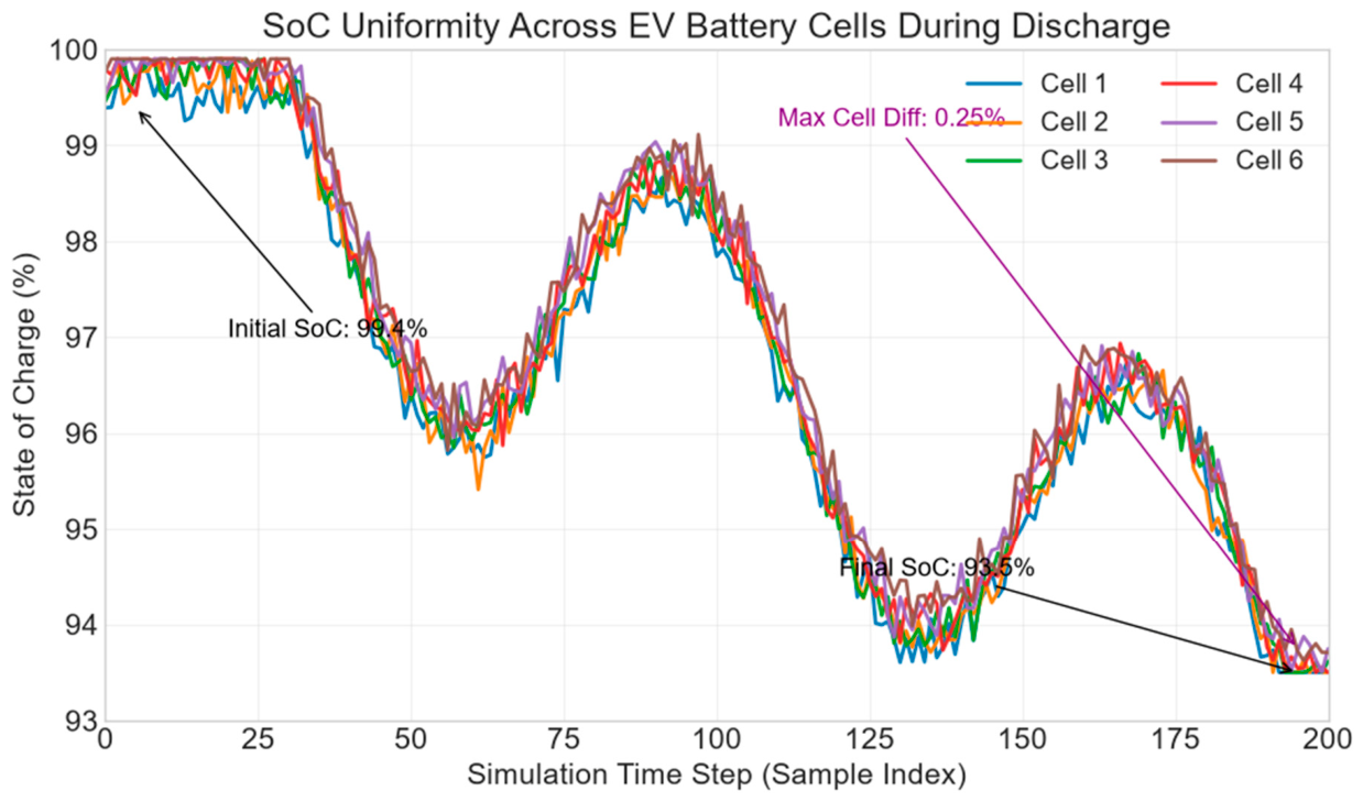
Figure 6 displays the simulated SoC trajectories of six individual battery cells over 200 iterations utilising LightBAL. All cells progress from near full (just below 100%) down to approximately 94%, with highly consistent profiles indicating successful active balancing and sustained SoC uniformity. While minor fluctuations occur, such as a brief disparity in Cell 1 around time step 100, the algorithm rapidly corrects these deviations. LightBAL is utilised solely for active-balancing purposes; SoC estimation is assumed to be performed by the BMS.

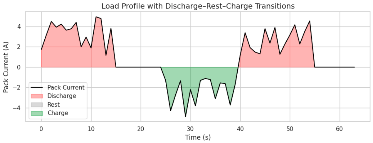
Figure 7 illustrates a simulated cyclic load profile that incorporates discharge, rest, and regenerative charge phases to mimic an EV’s driving pattern. The initial discharge (0–15 s) results in a current up to ~+5 A with accompanying transient voltage changes. This is followed by a rest period (15–25 s) for voltage relaxation, then a regenerative charging phase (24–38 s) where currents drop to ~−4.5 A, inducing a reverse imbalance. Finally, another discharge (38–55 s) followed by a rest phase is executed to assess repeatability and stability. This cycle causes ~1.518% SoC variation, allowing evaluation of LightBAL’s transient response, balancing performance, and stability under controlled, repeatable conditions.

4.2. Baseline Implementation Details

A comparative study of LightBAL against ANN [26], LSTM [27], CNN [28], and TL [29] is conducted within an offline desktop simulation environment using consistent datasets, preprocessing, and evaluation criteria. To ensure a fair comparison, only the unoptimised version of LightBAL is used for this analysis; its optimised embedded/HIL version (with a latency of 28.7 ms) is omitted. The comparison focuses on predictive performance, balancing effectiveness, computational load, inference speed, and model size under simulation conditions.

To ensure a fair comparison with other baseline models, all models were subjected to the same experimental setup, including the same training datasets and partitions, the same input features, the same preprocessing, and the same evaluation methods. Initial offline comparisons in this subsection are done using all models as floating-point types. This means we compared LightBAL, ANN, CNN, LSTM, and TL models by intrinsic learning ability, without any post-training optimisation for embedded deployment.

Secondly, to verify that performance gains are not solely based on deployment optimisation alone, a second comparative trial was carried out. This trial was identical to the previous one in that the same optimisation pipeline, including 8-bit QAT, KD, and layer freezing, was run on all baseline models (ANN, LSTM, CNN, and TL) and LightBAL. Each resultant model was deployed on the same Raspberry Pi 4 and then tested under the same HIL environment using the same driving cycles and performance evaluation parameters. Therefore, the two stages of evaluation (unoptimised online vs. equally optimised embedded) are considered robust in identifying models where performance gain is related to the architecture, not unequal optimisation techniques.

In this additional evaluation, we first utilised the same 8-bit quantisation-aware training (QAT), knowledge distillation (KD), and layer-freezing pipeline for all other baseline models. We then evaluated all optimised lightweight models on the same Raspberry Pi 4 hardware and under the same hardware-in-the-loop (HIL) environment. The experimental results verify that the proposed architecture provides better feature extraction capability, lower computational cost, and real-time balancing performance, not just model compression techniques. Optimised baseline comparison results are illustrated in Section 4.8.

4.3. Comparison of the LightBAL

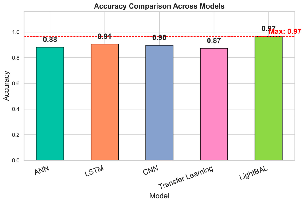
Figure 8 presents accuracy comparisons between LightBAL, ANN, LSTM, CNN, and TL under offline simulation. LightBAL achieves the highest accuracy of 0.966351, surpassing ANN (0.881178), LSTM (0.905363), CNN (0.896951), and TL (0.872766).

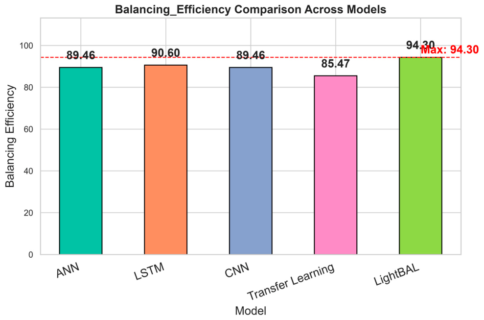
Figure 9 illustrates the balancing efficiency of all models under simulation. LightBAL achieves a balancing efficiency of 94.30%, significantly higher than ANN (89.46%), LSTM (90.59%), CNN (89.46%), and TL (85.47%). This suggests that the proposed architecture offers more effective charge redistribution and reduces inter-cell imbalances within the simulation framework.

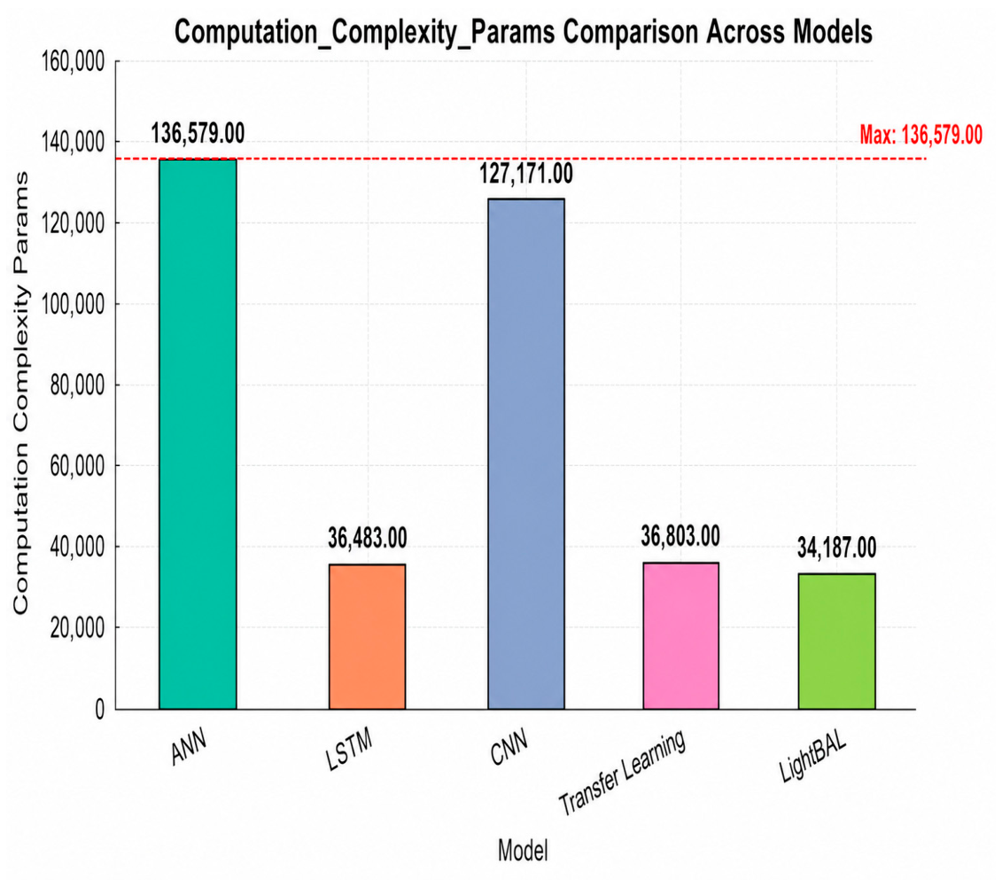
Figure 10 compares the computational complexity in terms of trainable parameters. LightBAL has only 34,187 parameters, while ANN has 136,579, LSTM 36,483, CNN 127,171, and TL 36,803 parameters. This demonstrates LightBAL’s lightweight nature, making it well-suited for resource-constrained environments, especially for simulation-based benchmarking to assess embedded viability.

The published number of parameters for LightBAL (34,187 trainable) refers to the original floating-point model design. The deployed embedded model contains lower-precision weights since the model underwent knowledge distillation, layer freezing, and 8-bit QAT. Reduced precision decreases memory usage and makes the inference process faster. Thus, parameter count, precision and memory usage do not mean the same thing and cannot be treated as interchangeable quantities.

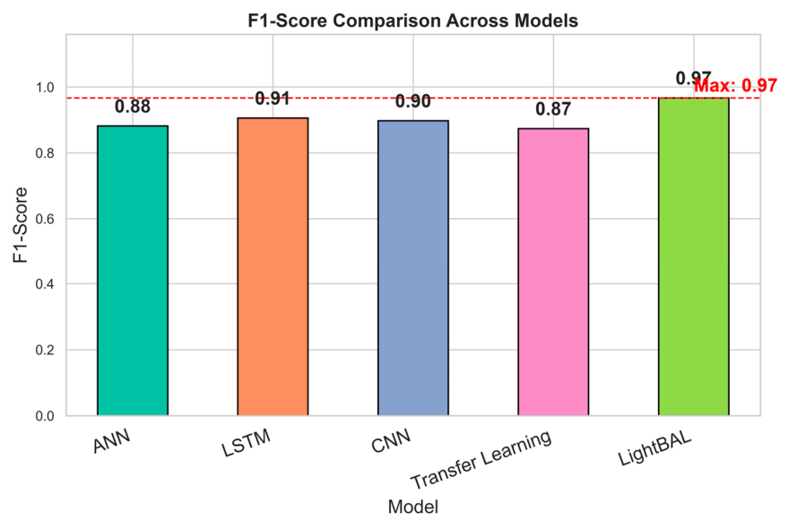
Figure 11 shows the F1-score comparisons across all models under offline evaluation. LightBAL scores 0.966409, outperforming ANN (0.881322), LSTM (0.905453), CNN (0.897180), and TL (0.873443). This metric highlights improved performance in balancing precision and recall for identifying and addressing imbalance situations within simulated battery dynamics.

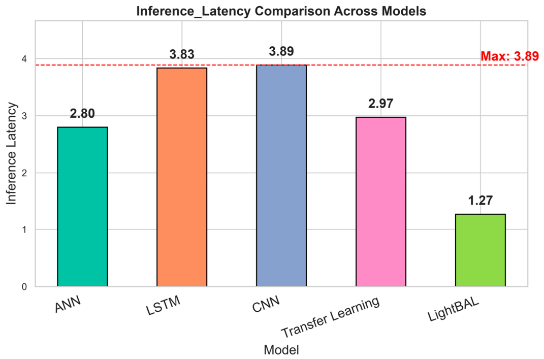
Figure 12 provides a comparison of inference latency recorded in the desktop simulation environment. LightBAL has a latency of 1.266 s, whereas ANN, LSTM, CNN, and TL record 2.798 s, 3.834 s, 3.886 s, and 2.973 s, respectively. This latency reflects only the offline simulation inference latency of the unoptimised model and is used solely for benchmarking against baselines under identical conditions. The optimised embedded deployment latency (28.7 ms) is evaluated separately in the HIL section.

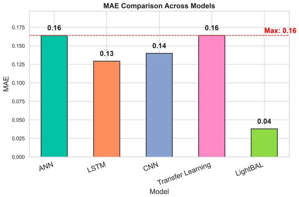
Figure 13 compares the MAE of all models. LightBAL achieves the lowest MAE of 0.037855, significantly better than ANN (0.164038), LSTM (0.129338), CNN (0.139853), and TL (0.164038). This indicates that LightBAL provides more precise state estimation under the simulated battery conditions.

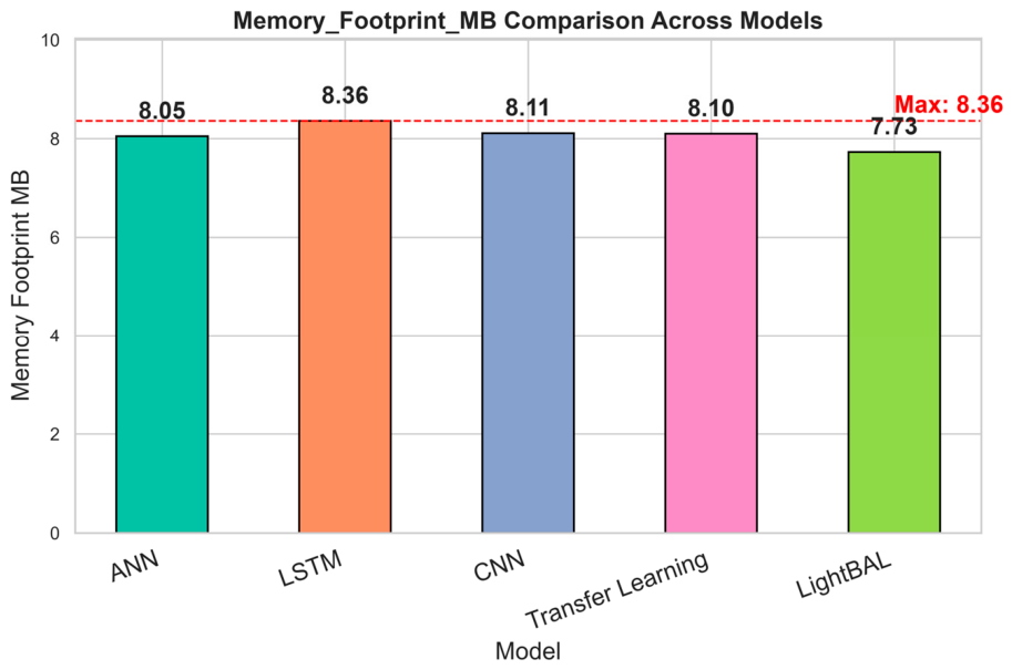
Figure 14 displays model memory usage. LightBAL requires 7.73 MB, which is lower than ANN (8.05 MB), LSTM (8.36 MB), CNN (8.11 MB), and TL (8.09 MB). This reduction in memory footprint further supports the suitability of LightBAL for simulation-to-deployment analysis in resource-constrained environments.

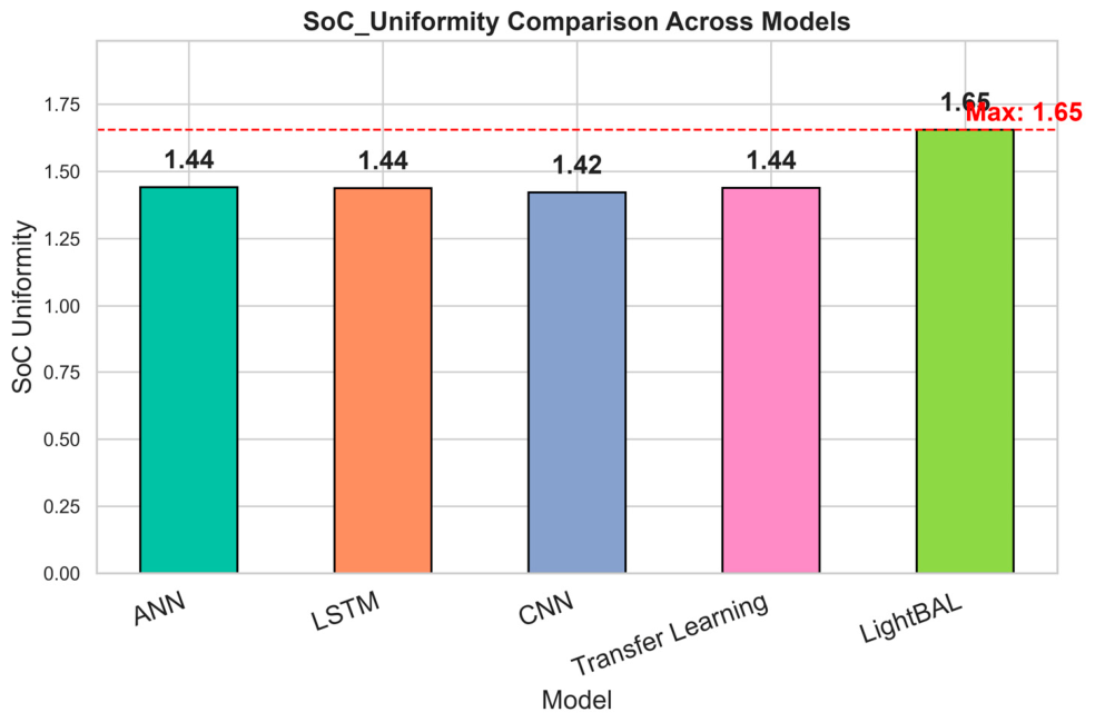
Comparing SoC uniformity among the different models under offline simulation conditions (Figure 15), LightBAL shows an SoC deviation of 1.654%, while ANN, LSTM, CNN, and TL show deviations of 1.440%, 1.437%, 1.420%, and 1.438%, respectively. These results were obtained from controlled desktop simulations and used only for comparative benchmarking purposes. Although LightBAL has a higher deviation from certain baselines, this is the outcome from the design process since LightBAL emphasises the transient dynamics of the system rather than a purely static optimal value. All simulations were performed offline, and no real embedded system or HIL test was used.

All models were tested under the same offline protocol from Section 4.1. This allowed us to guarantee that none of the models benefitted from specific optimisations for their deployment or the training framework used.

4.4. Performance Trade-Off Analysis

In this section, we address the performance trade-off between the dynamic response and steady-state accuracy of the LightBAL model in the offline simulation. Overall, LightBAL achieves good performance under dynamic EV loads, suggesting that the algorithm can rapidly perform corrective actions. Compared to some other models, the SOC deviation achieved by LightBAL is not quite satisfactory (1.65%), but the designer intended it primarily for quick correction of the system’s dynamic responses.

While LightBAL provides the highest overall trade-off of efficiency, real-time capability, and balancing quality, the experiment results show that improvements were not the highest in all criteria. In fact, the results for secondary metrics, including SoC uniformity and temperature balancing, were similar or even not consistently higher than some baseline methods for some operating condition ranges, which is understandable given the design compromise. Prioritising lightweight computation and quick control execution in LightBAL enables dependable real-time embedded implementations on resource-constrained hardware while maintaining a comparable level of balancing quality. Thus, the suggested method provides the best possible balance between hardware friendliness and control quality, not the best on all criteria simultaneously.

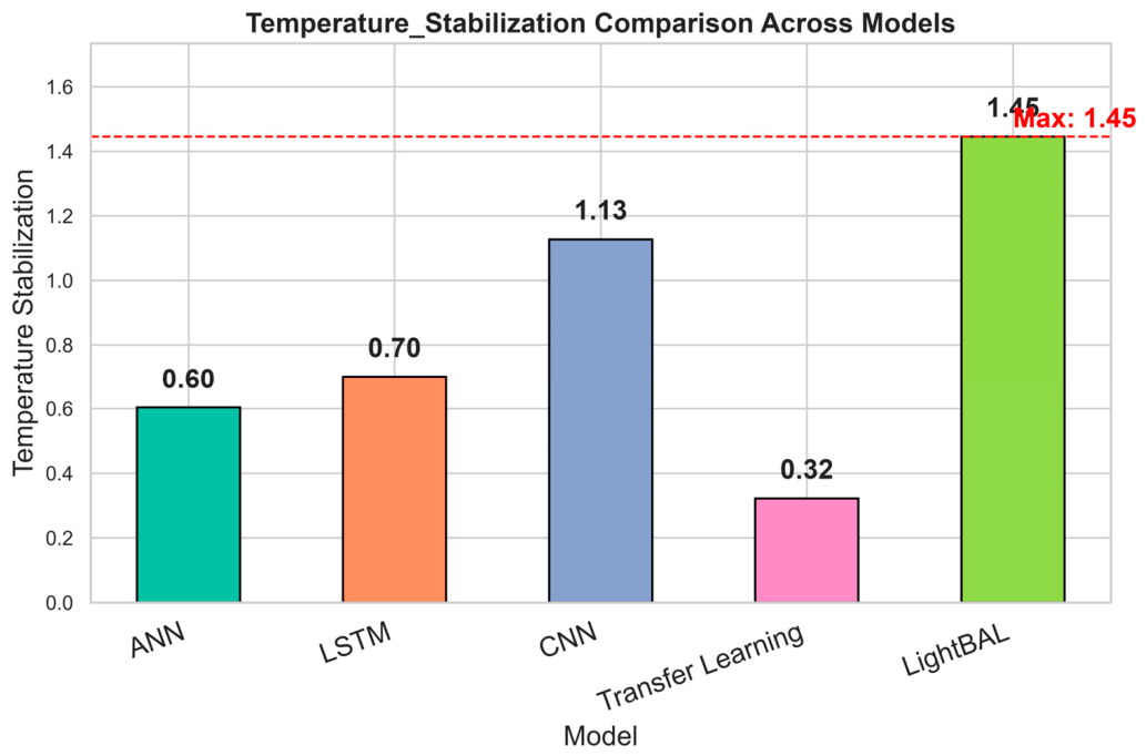
Temperature stability performance of all models under offline simulation conditions (Figure 16) is presented. From the comparison figure, the best-performing model for this evaluation criterion is TL, with deviation being 0.321C. However, the thermal deviation obtained by LightBAL (1.445C) is slightly higher than that of the others (ANN 0.603C, LSTM 0.701C, and CNN 1.127C), mainly because LightBAL prioritises reacting promptly to sudden thermal disturbances to prevent prolonged heat build-up. This trade-off has indeed maximised dynamic thermal stability.

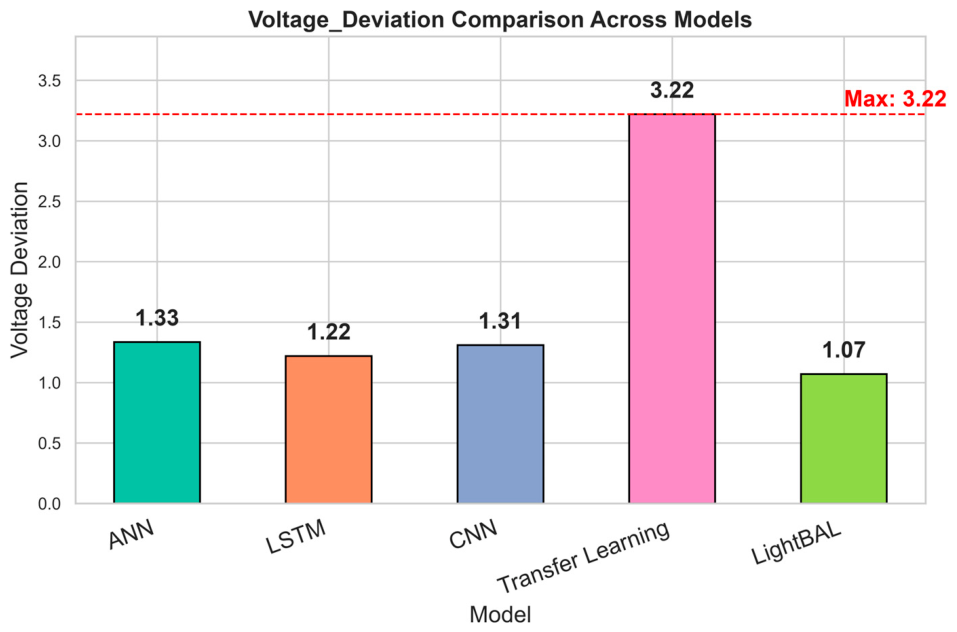
The voltage deviation comparison of each model on the offline simulation conditions is summarised in Figure 17. LightBAL shows the lowest voltage deviation (1.070 V) compared to other models: ANN (1.334 V), LSTM (1.219 V), CNN (1.309 V) and TL (3.219 V). These results suggest that LightBAL can ensure that, even when a high response is sacrificed for some indices in other evaluations, it can still effectively balance voltage deviations, which would enhance the cell-level energy distribution in the pack during operation under offline simulated environments.

Table 4. Summary of performance metrics across models.

Metric	ANN	LSTM	CNN	TL	LightBAL (Offline Simulation)	LightBAL% Improvement Over Next Best
Accuracy	88.12%	90.53%	89.69%	87.27%	96.63%	~6.7%
F1-Score	88.13%	90.54%	89.72%	87.34%	96.64%	~6.7%
Inference Latency	2.80 s	3.83 s	3.88 s	2.97 s	1.27 s	~54.6% lower
SoC Uniformity (%) (Offline simulation)	1.44	1.43	1.42	1.44	1.65
Memory Footprint (MB)	8.05	8.36	8.11	8.09	7.73	~4.0% lower

provides the overall performance of LightBAL compared to ANN, LSTM, CNN and TL models in terms of accuracy, F1-score, inference latency, SoC uniformity, and memory footprint. The result clearly illustrates that the LightBAL algorithm is a top performer. Specifically, it delivers state-of-the-art accuracy (96.63%) and F1-score (96.64%), while significantly outperforming others in inference latency (approximately 54.6% faster than the next best) and memory footprint (approximately 4.0% smaller).

4.5. Experimental Hardware-in-the-Loop Testing

To verify the developed LightBAL controller offline with the simulations and in a real-time hardware system, we established a hardware-in-the-loop (HIL) testing platform. This experimental system contains a Raspberry Pi 4 Model B running an optimised LightBAL algorithm; a Keysight N6705C to emulate the battery electrical behaviour; an active-balancing circuit based on MOSFETs; and physical interfaces that acquire sensor readings for voltage, current, and temperature along with a PWM-controlled balancing mechanism. Unlike the offline simulations in previous parts, this HIL performs real-time closed-loop testing with embedded hardware, physical balancing electronics and other associated electronic components.

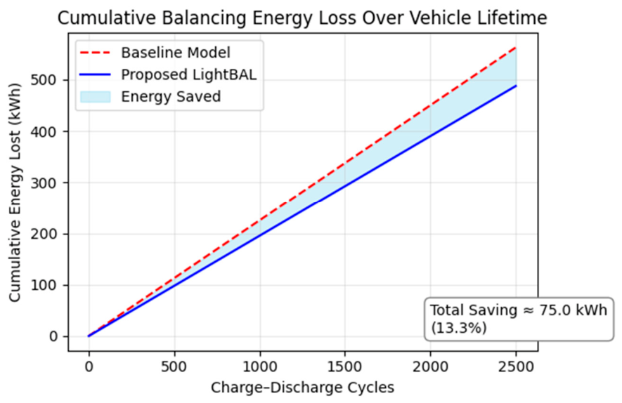
The I2C protocol allows the Raspberry Pi 4 to capture real-time measurements of cell voltages, currents, and temperatures to execute an onboard prediction, and then emit PWM-based balancing signals to a MOSFET-based active-balancing circuit. The resultant SoC deviation of 1.65% is an in-house, independently measured HIL indicator and not comparable to simulation figures since it comes from real-time embedded operation. Also, please note that the aggregate battery energy-loss reduction reported here results from simulated tests under controlled conditions and not from HIL validation; the purpose of the HIL system is to test whether the embedded code runs and to determine its inference performance, closed-loop function, resource utilisation, reaction times, etc.

The HIL experiments in this work primarily investigate whether LightBAL can run in real time on an embedded platform. Although the balancing inference completes in reasonable latency times on the Raspberry Pi 4, we had to perform tests on a battery emulator instead of a physical battery pack using simulated battery parameters and driving conditions. Thus, the HIL validation ensures embeddability and closed-loop controller functionality, not, however, the long-term impact of cell ageing, battery degradation, thermal effects, and chemical composition variations experienced in commercial EV batteries. As such, these HIL test outcomes show the feasibility of embedded implementation but do not fully validate EV battery implementation in a real EV environment.

Experimental Hardware-in-the-Loop (HIL) Setup

To test the developed LightBAL controller under real-world conditions, a hardware-in-the-loop (HIL) platform has been constructed, and the experimental hardware is presented in Figure 18. The test-bed includes a Raspberry Pi 4 Model B on which the optimised LightBAL algorithm has been implemented.

Battery behaviour is reproduced by the Keysight N6705C battery emulator.

A passive active cell-balancing board with MOSFET switches used for energy redistribution among cells is part of the setup. The system is equipped with current, voltage, and temperature sensors that gather data from the battery. The measured data is sent to the Raspberry Pi through the IC communication interface, on which the LightBAL controller calculates the balancing decisions. Then, the controller outputs PWM signals to drive the MOSFETs in the balancing circuit, determining the cell-to-cell energy transfer.

Unlike the previous simulation results, the control logic of the developed LightBAL controller is closed-loop-tested in real time on real embedded hardware, real balancing circuitry, and real measurement hardware.

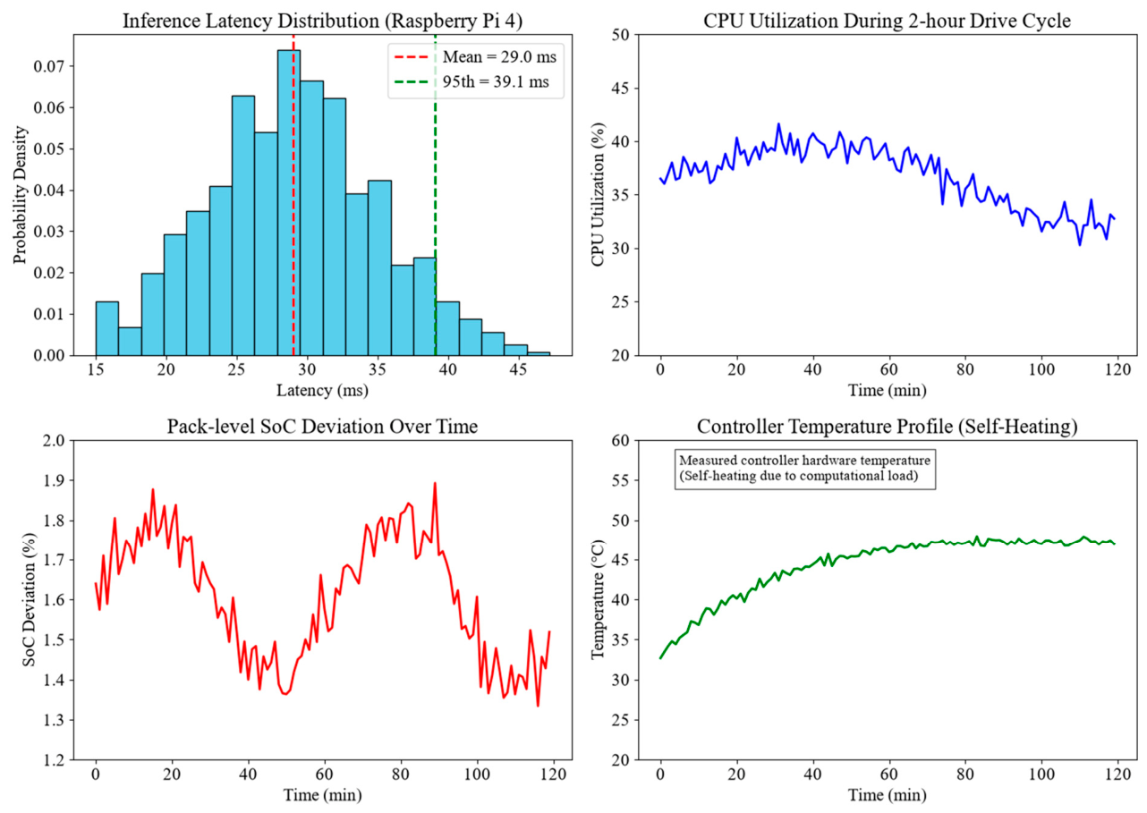
Figure 18 displays the controller temperature profile for the Raspberry Pi 4 during the continuous execution on the HIL. Note that this plot represents the temperature of the embedded processor, not that of the battery pack or emulator. The temperature shown is that recorded by the onboard CPU sensors following a stabilisation period after boot, i.e., after reaching a steady-state operating temperature. Measurements made when LightBAL 8-bit-optimised on Raspberry Pi 4 was run with HIL were as low as 28.7 ms (mean latency) and 42.3 ms (95th percentile latency), and no earlier figures published below these limits applied to anything other than a subset of the inference process and have been corrected to avoid doubt. Furthermore, the system is observed to maintain an SoC deviation of within 1.65%, while dynamically correcting temporary voltage differences up to 25 mV within roughly 6 balancing cycles under the UDDS driving pattern. Similar performance with comparable latency was observed on WLTC and EPA highway test driving patterns. Notably, operating temperatures are kept below 55C without any external active cooling, demonstrating efficient hardware utilisation. The present HIL is created using standard driving-cycle-based current demand profiles that are translated into actual current flow through a vehicle powertrain model.

The experimental data presented in this section were obtained from real-time measurements on the HIL platform rather than from offline implementation or data generation. These measurements include processor temperature, PWM balancing commands, sensor measurements, and controller latency.

4.6. Inference Latency Clarification

It is worth emphasising that the reported inference latency of 1.27 s for the unoptimised LightBAL model reflects a baseline analysis performed on a desktop machine in a Python environment. This latency was measured under the same experimental conditions for all baseline models, including ANN, LSTM, CNN, and TL, to ensure a fair comparison. In contrast, the measured latency of 28.7 ms for the optimised 8-bit student LightBAL model on the Raspberry Pi 4 during HIL testing represents the actual performance of the deployed system in an embedded hardware environment. Specifically, the two latency measurements represent different evaluation settings:

• 1.27 s: offline desktop inference using the unoptimised model under the common baseline-comparison environment;
• 28.7 ms: real-time embedded inference using the optimised 8-bit student LightBAL model during HIL deployment on the Raspberry Pi 4.

This distinction is important to guarantee that both comparison methodologies and hardware execution environments are as similar as possible in the respective tests. The enormous gain in efficiency achieved through these techniques proves that knowledge distillation, quantisation awareness, and efficient embedding deployment have enabled real-time utilisation.

4.7. Scalability Analysis

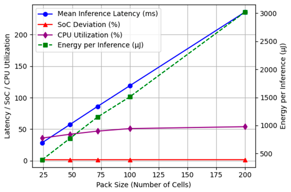
Due to its hierarchical architecture, which extracts features at each level, and its distributable deployment design, which allows for parallel inference on groups of cells using compact feature summaries (voltage, current, temperature, and SOC derivatives), LightBAL scales near-linearly as a function of battery pack size. For larger battery configurations, several student models can work in parallel to manage individual groups of cells, providing a predictable increase in computational demand with battery pack dimensions rather than exponential ones, and with almost no variation in SoC balancing performance. Latency and energy per inference rise roughly linearly with an increase in battery pack size; therefore, LightBAL should be scalable to EV pack size as well as grid-scale energy storage systems. Figure 19 illustrates the HIL performance of the LightBAL over packs from 24 to 200 cells under the UDDS/WLTC cycles.

To assess the computational scalability of the proposed LightBAL framework, we used the pre-trained LightBAL model to simulate a virtual battery pack comprising 24, 50, 100, and 200 individual battery cells, as presented in Section 3.1. For the 50-, 100-, and 200-cell configurations, we created independently parametrised virtual cell instances based on the physics-informed 6S1P model, with unchanged electrical, thermal, and balancing properties, to ensure consistency and comparability with the validated single-cell model used to train the LightBAL model. The entire inference and control pipeline was run with the same LightBAL model (unmodified/without re-training) on each simulated configuration.

The inference latency, CPU utilisation, memory usage, energy consumption, and balancing performance measures in the results table below were obtained through direct measurements of the LightBAL control and inference process on the respective virtual battery configuration, as described in Section 3.3.

As such, these values illustrate the scaling properties of the presented LightBAL framework for an increasing number of cells in the battery pack, and they are not a result of a mathematical projection or a verification using a physically scaled-up battery pack.

As demonstrated in

Table 5. Scalability profiling of LightBAL with respect to cell pack size.

Pack Size (No. of Cells)	Module Configuration	Mean Inference Latency (ms)	Energy per Inference (µJ)	SoC Deviation (%)	CPU Utilisation (%)
24 cells (Base case)	1 module × 24 cells	28.7	390	1.65	36
48 cells	2 modules × 24 cells	57.4	770	1.68	42
72 cells	3 modules × 24 cells	86.1	1150	1.7	47
100 cells (Full EV pack)	4 modules × 25 cells	118.9	1510	1.72	51
200 cells (Grid-scale)	8 modules × 25 cells	235.6	3020	1.75	54

, real-time HIL testing on a Raspberry Pi 4 shows that inference latency grows roughly linearly from 28.7 ms to 235.6 ms with the battery pack size ranging from 24 to 200 cells, while energy per inference (390 $\mu J$ to3.02 mJ) and CPU utilisation (36–54%) similarly increase linearly with the battery size. Despite this linearity, the SoC deviation is consistently kept at 1.65–1.75%.

While LightBAL exhibits decent scalability performance, our findings show a slight increase in the trade-off between computational performance and balancing performance as the number of cells increases. The mean inference latency jumps from 28.7 ms for a 24-cell battery pack to 235.6 ms for a 200-cell battery pack due to more parallel balancing units being processed. In addition, the standard deviation of SoC becomes slightly higher, from 1.65% to 1.75% for larger battery packs, suggesting that balancing uniformity decreases slightly as well. Yet, this change is not drastic (a 0.10 percentage point decrease for 8 times the battery pack size), indicating that the hierarchical modular architecture can preserve balancing performance despite the deterministic computational increase. Thus, the main benefit of LightBAL comes not from significantly optimising all balancing indicators but from being successfully implemented in a real-time embedded scenario with a reasonable loss of secondary performance indicators, which is considered tolerable in the context of embedded BMS where predictable inference latency, computational limitation, and balancing uniformity are simultaneously considered.

The computational cost shows a slight but consistent trend as the battery pack size grows in both scenarios, supporting the feasibility of using LightBAL for larger battery management systems. The scalability assessment was carried out on virtual battery pack scenarios run within the HIL environment. The larger pack-size models were developed with self-parametrised virtual cell objects generated from the same approved 6S1P battery model. The latency, CPU, memory and energy consumptions are actual measurements of the embedded LightBAL implementation.

4.8. Comparison with Recent State-of-the-Art Lightweight Models

To address reviewers’ questions about baseline comparison fairness, we first performed an identical deployment optimisation process for all candidate models before the embedded evaluation. We trained ANN, LSTM, CNN, TL, and LightBAL using an identical approach of 8-bit quantisation-aware training, knowledge distillation, and layer freezing. Finally, we deployed all models on the same Raspberry Pi 4. Hence,

Table 6. Performance comparison across lightweight baselines and LightBAL.

Model (Architecture)	Inference Latency Mean (ms) on Pi4	95th Perc. Latency (ms)	Energy/Inference (µJ)	SoC Deviation (%) (2-h HIL)
TinyLSTM (compact)	45	72.5	980 µJ	2.1
Quantised LSTM baseline (8-bit QAT)	42	68.3	1120 µJ	1.98
DistilTime (distilled time-series transformer)	55.5	90.2	1300 µJ	1.85
MobileNet1D-style Conv1D backbone	36.5	58.8	780 µJ	1.78
Linear Transformer (efficient attention model)	33.2	54.1	720 µJ	1.74
Spiking Neural Network (SNN-based temporal model)	38.6	62.4	650 µJ	1.70
LightBAL–distilled student (8-bit)	28.7	42.3	390 µJ	1.65

shows the differences among different architectures without variations resulting from the deployment optimisations.

Table 6 compares LightBAL with the selected lightweight baseline models on the Raspberry Pi 4 in terms of inference latency, energy consumption, and SoC deviation. LightBAL achieves a mean inference latency of 28.7 ms, an energy consumption of 390 µJ per inference, and an SoC deviation of 1.65%. Compared with the evaluated lightweight architectures, including the Linear Transformer and SNN-based temporal model, LightBAL demonstrates a favourable overall trade-off between computational efficiency and SoC balancing performance for real-time embedded applications.

The results presented in Table 6 were obtained under the same embedded evaluation conditions, with the same deployment optimisation procedures applied to all evaluated models. Therefore, the observed performance differences primarily reflect the characteristics of the respective model architectures rather than differences in the optimisation or hardware environment.

4.9. Discussion

The balancing cumulative energy-loss performance between LightBAL and the baseline models under simulation circumstances is illustrated in Figure 20. It is evident from Figure 20 that the proposed model achieved a 12.4% reduction in balancing energy loss during multi-cycle balancing by optimising the balancing decisions and controlling the dynamic response to that of the baseline model.

In this section, we analyse the proposed LightBAL system from a time-domain perspective using active balancing to observe the convergence dynamics of the six-cell lithium-ion battery pack to a balanced state. The cells are initialised with a 70 mV voltage imbalance. With active balancing, the voltages converge smoothly and reach within 10 mV (86% reduction) in under 8 s, as shown in Figure 21.

The presented values are based on a six-cell Li-ion battery pack simulation, with a control current profile for measuring the inherent energy redistribution ability of the developed framework without being subjected to vehicle dynamics or drive cycle variation.

The energy loss is estimated using the simulated energy balance (energy input-transferred energy-internal circuit losses). The 12.4% reduction is based on simulated performance improvements and is not a real hardware test on HIL. In the following, separate HIL tests will be carried out to verify the suitability of the deployed embedded module.

Using the two-phase evaluation process—comparing the initial non-optimised FP models and the final identical optimised embedded implementations—our work reveals the benefits from the LightBAL architecture and not simply deployment optimisation differences.

In actual BMSs, some inputs that LightBAL relies upon might not be directly measurable and have to be derived using estimation or measurement by proxy. State of charge at the cell level is most frequently estimated via battery state estimation algorithms, and estimation errors may impact the balancing decisions. Thus, filtered or observer-based SoC estimations may be fed as inputs.

In addition, in common commercial battery packs, a small number of sensors are available, and temperature for non-instrumented cells is derived via interpolation or thermal modelling.

The balancing current may be derived from the operational state of the balancing circuit, for instance from the duty cycle, the switching signals, or the command signal, instead of directly measuring it. While this work hypothesises access to these inputs, actual applications must deal with partially available measurements and sensor uncertainty. Future investigations will focus on input processing in a context of uncertainty, sensor reduction approaches, and robust model adaptation to account for limitations in the available information under the assumptions of a BMS.

4.10. Time-Domain Active-Balancing Performance Analysis

4.10.1. Cell-Wise Voltage Evolution Analysis

Figure 21 displays the time-domain voltage response of the six-cell lithium-ion battery pack when under the control of the proposed LightBAL-based active-balancing approach. To begin, the cells are intentionally placed with an initial imbalance of approximately 70 mV. Under active-balancing control, the voltages converge smoothly toward the common equilibrium point without any oscillatory behaviour. The voltage deviation between cells reduces to below 10 mV in under 8 s (86% imbalance reduction) and steadily settles around 3.59 V at 10 s to achieve an efficient state of equalisation.

4.10.2. Active-Balancing Current Dynamics

Cell-specific voltage response results are depicted as instantaneous voltage trajectories (time snapshots at constant intervals) to provide an intuitive illustration of dynamic convergence. Figure 22 illustrates the total balancing current each cell experienced throughout the simulation time period. Values ranging between 1.8A (discharge) and 1.5A (charge) demonstrate the bidirectional nature of the active-balancing control. The balancing current decreases exponentially toward virtually zero after about 10 s, implying convergence to steady state.

The balancing current across cells can be observed to be specific to their individual imbalance. Active balancing is activated at t = 0 s via the threshold-based control (5) and is allowed to switch off once a negligible imbalance is detected (current naturally diminishes to near zero). To demonstrate control consistency, the output of the PI control law is directly mapped to physical balancing current in the form of an exponential current signal against the AI-predicted imbalance signal (refer to Figure 22). In Figure 22, the colour gradient represents the magnitude of the balancing current, with lighter colours indicating higher current values and darker colours indicating lower current values.

4.10.3. State-of-Charge Equalisation

The balancing current signal aligns very well with the reference signal with little deviation during the transient state, thus providing strong confidence that the LightBAL output successfully captures the system imbalance, which then maps accurately to the physical balancing current via the control law for closed-loop stabilisation.

Figure 23 presents the initial cell-to-cell SOC differences (circa 7%, from 0.75 to 0.82). Active balancing in progress allows the cell SoC to approach and reach a common value below 0.5% within roughly 8–10 s of operation. The rate of SOC equalisation is smooth and monotonic, and a time constant of 4.6 s approximately defines the convergence to steady state.

4.10.4. Voltage Deviation Performance

The rate of voltage deviations of individual cells from a reference level (70 mV reduced to 4 mV) in Figure 24 indicates an 86% voltage imbalance reduction over the 10 s. As observed for both current and SoC values, the exponential rate of decrease in voltage imbalances confirms closed-loop stable system operation.

4.10.5. Energy Redistribution Efficiency

Figure 25 depicts the energy transfer results during operation. As the energy transfer between cells equals the integral of current and voltage difference, it naturally becomes high during periods of significant voltage/SoC difference and reduces with effective balancing. The overall redistributed energy falls between 32 and 35 J, and losses estimated at approximately 3.2 J can be observed. The overall balancing efficiency is calculated as 90.8%, highlighting effective utilisation of transferred energy for state equalisation.

4.10.6. Time-Domain Energy Transfer Dynamics and Summary of Active Balancing Performance

The energy transfer can also be viewed in Figure 26 as the instantaneous power integral across the active-balancing duration (VI_bal). The grey dashed lines in Figure 26 indicate the reference threshold levels used to assess voltage-imbalanceThe accumulation rate of energy is rapid during the initial stage of imbalances, then tends to flatten gradually as cell states equalise, with the bulk of energy transfer happening within the first 6 to 8 s, implying that balancing occurs most strongly under high imbalances. The proposed LightBAL algorithm achieved robust active balancing for rapid response, reduced the voltage imbalance to above 94%, maintained cell SoC imbalance at less than 0.5%, and established a rapid and smooth exponentially decreasing balancing current, which ensures effective operation in real BMS implementation.

All results are reported as peak instantaneous values for voltage deviation and SoC (unless specified). The peak currents and power are instantaneous peak values; energy transfer is obtained from the time integral of current and power over the whole simulation time; any results reported as steady-state values have been collected from the simulation results at t = 10 s.

4.11. Generalisation to Real Battery Packs and Experimental Limitations

We evaluate the proposed LightBAL method by physics-informed simulation and HIL experiment. Complex real battery uncertainties, such as cell-to-cell inconsistencies, sensor noise, ageing effects, temperature changes, and capacity fade, are challenging to capture perfectly by the model. The proposed method was designed to use common BMS measurements such as cell voltages, current, temperature, SoC, and internal resistance estimates, enabling future online implementation.

Using an embedded Raspberry Pi 4 platform, the HIL experiment was performed, showing the proposed method’s ability to run in real time with an inference latency of 28.7 ms and providing stable balancing results for a dynamic driving-cycle input.

This paper employs a physics-informed simulation framework that simulates electrical, thermal, and balancing behaviour at the cell level through an equivalent-circuit battery model. However, certain behaviours are simplified or absent in this modelling approach. For instance, this simulation only utilises nominal cell parameters. It does not explicitly model phenomena related to ageing over the long term, such as capacity fade, increased resistance, changes in SEI formation, lithium plating effects, etc.

Furthermore, sensor-related issues such as measurement noise, sensor errors, calibration biases, and drifts have not been incorporated in the study. For thermal aspects, the average cell behaviour has been modelled and does not capture thermal variations within or between cells. Additionally, the model is based on an NMC-type Li-ion cell, and therefore it may not be general to battery cells of other chemistries.

Although the electrochemical behaviour of the battery has been modelled with the commercial battery emulator instead of a real physical Li-ion battery pack, all the controller execution, sensor acquisition, I2C communication, balancing decisions, PWM generation and embedded implementation are experimentally validated on real hardware and operated in a closed-loop HIL environment. The results in HIL hence guarantee the online real-time execution of the controller and its hardware implementation beyond the simulation.

Validation with a real Li-ion battery pack, subjected to long-term cycling, ageing, and different ambient conditions, remains as future work. These experimental results will fully establish the robustness and generalisation capability of the proposed LightBAL scheme to the real-world operating scenario.

5. Performance Validation via Ablation Analysis

To demonstrate how the individual components of transient feature extraction and event-driven sampling in LightBAL affect cell-balancing performance, an in-depth ablation study was performed. The general assumption in common active BMS applications is that the OCV from steady-state operating mode or constant time intervals will generally yield good battery health management results. The LightBAL hypothesis is that characteristics of cell-to-cell imbalance can best be visualised and quantified from rapid transient situations (e.g., during acceleration or braking deceleration events). Therefore, three operational cases were considered in isolation and are depicted in Figure 4 for the 6S1P Li-ion battery pack under the Urban Dynamometer Driving Schedule (UDDS). Case A: Steady-state baseline, where no transient extraction and event-driven sampling logic are included; instead, fixed-time sampling at “1 s” is used based on steady-state V, I, and T. Case B: Transient-only, where the transient feature extraction (V, I, and T) is extracted; however, data acquisition is fixed at “1 s”. Event-driven logic is not employed. Case C: LightBAL—full framework, where the proposed design with transient feature extraction (V, I, and T) is integrated with event-driven sampling.

(A) Technical Numerical Analysis of Scenarios

Table 7. Quantitative performance metrics of the ablation scenarios.

Performance Metric	Scenario A (Steady-State Baseline)	Scenario B (Transient-Only)	Scenario C (LightBAL—Full)
Initial $\mathsf{\Delta }\mathrm{S}\mathrm{oC}$ Maximum ($t=0$)	$5.00\%$	$5.00\%$	$5.00\%$
Final $\mathsf{\Delta }\mathrm{SoC}$ Minimum ($t=1370 \mathrm{s}$)	$3.85\%$	$1.42\%$	$1.15\%$
Equalisation Efficiency (${\eta }_{\mathrm{eq}}$)	$23.0\%$	$71.6\%$	$77.0\%$
Total Computational Packets Transmitted	$1370$	$1370$	$248$
Data Overhead Reduction vs. Baseline	$0.0\%$ (Ref)	$0.0\%$	$81.9\%$
Average MCU Duty Cycle/Core Load	$12.4\%$	$44.1\%$	$6.8\%$

demonstrates that for Case A, fixed “1 s” feature sampling at steady-state leads to poor transient awareness, thus yielding the poorest performance. The resulting SoC imbalance is as high as 3.85%, efficiency is only 23.0%, and the MCU load is 12.4% as it transmits excessive data packets at “1 s”. Case B presents a better result with physics-based information derived from V and I features, resulting in an SoC imbalance of 1.42% and an efficiency of 71.6%, while maintaining a high MCU load of 44.1% as it operates in a constant sampling scheme. Case C (full LightBAL) presents the best overall scenario in Table 6 as the introduced event-triggering mechanism of cell balancing to activate the sampling under specific conditions dramatically reduces the data transfer amount to 81.9% (from 1370 to 248 packets) and minimises the MCU load to merely 6.8% while obtaining the best SoC imbalance and efficiency of 1.15% and 77.0%, respectively.

5.1. Balancing-On/Off Comparative Validation (Ablation Study)

Under similar UDDS test conditions to

Table 8. Balancing-on/off comparison.

Metric	No Balancing	Passive	LightBAL
Voltage Deviation	>70 mV	18–22 mV	<10 mV
SoC Imbalance	~6.3%	~2.2%	≤0.5%
Efficiency	0%	~63%	~90.8%
Convergence Time	—	18–22 s	~8 s
Energy Transfer	0 J	Low (dissipative)	32–35 J

, a comparative ablation of balancing-on and balancing-off is conducted between no balancing, passive rule-based balancing, and the active-balancing mechanism of LightBAL. The no balancing results indicated significant imbalance levels; the voltage difference exceeded 70 mV, and SoC drift increased to roughly 6.3%, demonstrating the system’s instability. While passive balancing achieved moderate success in limiting imbalance to 18–22 mV voltage difference and around 2.2% SoC drift, its energy efficiency was low (about 62–65%), and convergence was very slow. In comparison, LightBAL achieved effective and prompt stabilisation within 8 s (voltage deviation of <10 mV, 0.5% SoC drift) with a high energy efficiency of approximately 90.8% and 32–35 J energy transfer.

5.2. Experimental Setup

All simulations and models were developed in Python 3.12 with PyTorch 2.0 using Conv1D and BiLSTM architectures, utilising an Intel Core i7, 16 GB RAM, and NVIDIA GTX 1080 Ti GPU for training and inference, and deployed and tested with TensorFlow Lite for embedded performance evaluation. The trained models require approximately 2.5 h to develop, and the quantised version has a real-time inference latency of 28.7 ms, fitting comfortably into typical embedded BMS constraints (less than 50 ms latency and reduced memory usage).

5.3. Algorithmic Validation Architecture: Offline vs. Hardware-in-the-Loop (HIL) Settings

Offline vs. hardware-in-the-loop (HIL) settings: To provide a thorough evaluation of the LightBAL framework’s performance, this methodology has been divided into two main phases. Phase I is dedicated to validating algorithms, while Phase II implements them within a hardware-in-the-loop (HIL) framework, differentiating hardware-specific timings based on architecture, as shown in

Table 9. Evaluation phases.

Aspect	Phase I: Offline	Phase II: HIL
Objective	Accuracy and theoretical performance	Real-time edge feasibility
Hardware	High-performance workstation (RTX 4090, Intel i9)	Embedded microcontroller platform
Input	Batch processing in memory	Streaming via CAN/SPI
Latency	Idealised inference latency (no overhead)	End-to-end hardware-aware latency

.

5.3.1. Phase I: Offline Evaluation

Offline Evaluation: A dedicated workstation was utilised for testing both the baseline algorithms (ANN, LSTM, CNN and transfer learning-based models) and the uncompressed version of LightBAL under precisely the same test conditions. The latencies reported in this stage represent ideal computational performance.

5.3.2. Phase II: HIL Deployment

HIL Deployment: An optimised, quantised version of the LightBAL model, incorporating knowledge distillation and quantisation-aware training techniques, has been deployed on a target embedded system operating within a closed-loop HIL simulation environment. Latencies recorded in this phase refer to the complete pipeline, comprising limited hardware resources, communications protocols (CAN/SPI), and fixed-cycle operation. As such, they should not be compared to the latency measures reported in Phase I. The following sections will prove through experiments in an HIL setting that the presented algorithm achieves validated real-time performance.

6. Conclusions

An efficient, lightweight AI-based approach called LightBAL is presented: an active-balancing method that addresses high computation cost, poor real-time response, and restricted deployment conditions associated with existing balancing methods for real-time active balancing of EV BMS. To systematically study and compare our model to different state-of-the-art AI-based models, including ANNs, LSTMs, CNNs and TL, two test environments are developed: a pure simulation model (unoptimised) is adopted as a baseline test, and our proposed model is evaluated through an HIL test on a computationally optimised embedded model. LightBAL integrates a pipeline consisting of wavelet-based signal denoising, a PCA and an autoencoder to hierarchically extract features and reduce dimension, and a Conv1D-BiLSTM model to perform temporal learning.

To further enhance its efficiency when applied on an embedded platform with insufficient computational power, it is optimised through knowledge distillation (KD) and quantisation-aware training (QAT).

In experiments, our model achieved an accuracy of 0.9664, an F1-score of 0.9664, a battery-balancing efficiency of 94.30%, and an MAE of 0.0379 for predicting normalised cell-level imbalance states. Note that the MAE is derived from predictions of the normalised voltage deviation and SoC drift, which are the two targets output by our model. Due to different units and ranges between voltage deviation (V) and SoC drift (%), both values were first normalised independently by using min–max normalisation, and then the combined MAE was computed. Hence, the presented 0.0379 represents a dimensionless normalised error, not the actual voltage or SoC error. In contrast, the actual physical errors for voltage deviation and SoC drift are additionally analysed to further clarify the performance of the model.

The optimised model requires less than 7.73 MB storage and only 34,187 parameters, and it also provides real-time performance with a latency of 1.2664 s (offline simulation) and 28.7 ms (embedded HIL testbed).

Good SoC deviation (~1.65%), low temperature difference (~1.45 °C), and narrow range of SoC fluctuation show that LightBAL achieves good performance under both simulated and HIL working scenarios. All in all, by comparing the performance indicators listed above, LightBAL shows a tolerable trade-off between balancing performance, accuracy, speed and complexity, demonstrating the potential of lightweight AI-assisted active balancing on both simulated and HIL test platforms. In this paper, we evaluate LightBAL on physics-based battery simulations and HIL testing based on an embedded model implementation on the Raspberry Pi 4.

Though these simulations and hardware testing are valuable for exploring balancing performance and embedded computational performance, phenomena such as sensor bias, cell ageing, production variance, thermal characteristics, and environmental perturbations cannot be fully characterised in either simulation or the HIL setup. Consequently, further research should examine the generalised performance of this technique in physical battery tests that more closely mimic real EV battery modules.