Early Prediction of Commercial Energy Storage Battery Cycle Life Based on Health Features and Transfer Learning

Abstract

As the application scale of battery energy storage gradually increases, the accurate prediction of the remaining service life of large-capacity energy storage batteries is crucial for high-quality development in this field. To address the issues of insufficient reliability and poor generalization in large-capacity energy storage battery life prediction, a deep learning framework based on a long short-term memory (LSTM) neural network is developed. Early aging data from the first 150 cycles is used for the model, with outliers removed and noise reduced through Savitzky–Golay (SG) filtering. Data normalization and a sliding window method are employed for training. The model is validated on two batches of large-capacity batteries under GB/T 36276-2023 conditions at 25 °C and 45 °C, achieving the root mean square errors (RMSEs) of 0.86% and 0.50%, respectively, over 1000 cycles. Additionally, the method is tested on small-capacity batteries from an MIT dataset, achieving an RMSE of 4.3%. A transfer learning module fine-tunes the model using cycles 151–300, reducing RMSEs to 0.18%, 0.10%, and 3.1% for the three battery sets. This enhances the model’s generalization and offers a practical solution for life prediction in battery inspection and evaluation.

1. Introduction

Energy storage batteries are widely utilized in various fields, including new-energy vehicles, military communications, and aerospace. They have several advantages, including high energy densities, long lifespans, and low self-discharge rates [1,2,3,4]. However, complex side reactions occur within and outside the battery during repeated charging and discharging cycles, resulting in aging. This results in a decrease in battery capacity and voltage [5,6]. Moreover, extensive research has confirmed that the probability of accidents occurring with aged batteries is higher than with new batteries [7,8]. The state of health (SOH) of a battery is an important indicator of cycling performance [9,10,11]. The SOH is typically defined as the ratio of the original capacity of a battery to its current capacity. When the capacity of the battery drops to 70–80% of its initial capacity, it is considered that the end of its lifespan has been reached [12]. In the energy-storage market, aging tests must be conducted under unified standards to evaluate the cyclic performance of different battery products. However, these tests often require significant time. For example, under the test conditions specified in the standard GB/T 36276-2023 [13], which include 25 °C, constant power full charge and discharge, and 1000 cycles, it usually requires more than half a year for the entire test to be completed by a battery. This significantly extends the time required for a product to enter the market. Accurate and rapid methods for predicting battery life are of great significance for addressing the issue of the prolonged duration of traditional life tests. By reducing the detection time through life prediction, not only can the efficiency of battery evaluation be improved, but the rapid iteration of battery research and development can also be promoted.

Currently, the prediction of the remaining useful life (RUL) of lithium-ion batteries is mainly categorized into two types: model-based prediction methods and data-driven prediction methods [14]. Model-based prediction methods include empirical [15], physical, and electrochemical approaches. Capacity fade curves were fitted and predicted by empirical models based on influencing factors such as temperature and state of charge (SOC). Batteries are simplified into equivalent circuits of electronic components such as resistors and capacitors using physical models, with the lifespan predicted through the identification of parameter changes in these components as the battery ages. Aging was simulated using electrochemical models based on the internal reaction mechanisms and material parameters.

Data-driven prediction methods do not require the establishment of concrete models. Instead, machine learning algorithms are used to intelligently learn and capture the correlation between aging features and health status. These methods have been widely studied in recent years owing to their high prediction accuracy and simple modeling processes. Battery-capacity fading is classified as nonlinear time-series data, and recurrent neural networks (RNNs) are considered suitable for predicting unknown sequences [16]. As a variant of RNN, the gate structure in LSTM networks is effective in addressing the long-term dependency and gradient explosion problems associated with RNNs [17,18]. A hybrid model based on deep convolutional neural networks and LSTM with Bayesian optimization (BO-DCNN-LSTM) was proposed for RUL prediction [19]. The combination of the lightning search algorithm (LSA) with LSTM was proposed by Reza et al. [20], who utilized the mathematical system sampling (SS) method to identify features and train models, which were verified on the NASA dataset. An LSTM model for predicting the SOH was proposed by Li et al. [21] based on a joint denoising model of complete ensemble empirical mode decomposition with adaptive noise (CEEDMAN) and SG filtering, and was verified on the CALCE dataset. Xing et al. [22] designed an interpretable composite health indicator, GPHI, via improved genetic programming. Only two cycles of early discharge voltage curves are required to define mathematical aging features, achieving low computation costs and stable early-life prediction accuracy on the MIT LFP dataset. Hou et al. [23] developed a physics-enhanced Transformer integrating embedded LSTM and wavelet preprocessing. Physical degradation equations were embedded as consistency loss during training, and selective transfer learning enabled cross-chemistry prediction with outstanding robustness under limited training samples. Wang et al. [24] put forward a cross-protocol PINN architecture consisting of two sub-networks. Automatic differential physical constraints and monotonic loss guarantee physically reasonable SOH outputs, and the framework achieves outstanding generalization across diverse battery chemistries and charging strategies with minimal prediction error on large-scale tests. Despite the progress of the above Transformer, physics-informed and interpretable prediction methods, most existing approaches demand abundant full-lifecycle cycle data for training and lack targeted optimization for early-stage aging prediction under unified national energy storage test standards, which restricts their practical deployment in commercial scenarios for rapid battery evaluation.

Although numerous studies on the life prediction of energy storage batteries currently exist, the existing research still faces challenges in commercial applications. On the one hand, a large number of input cycles are required in existing research, which includes complex secondary features such as dV/dQ peaks and dQ/dV [25]. This is feasible for obtaining high-quality data from small-capacity batteries tested in laboratories. However, in commercial testing processes where numerous parallel tests and large battery capacities exist, a vast data volume is often accompanied by noise interference. This complicates the commercialization of existing life prediction methods. On the other hand, models are built by existing research based on the aging test data of multiple batteries of the same model. However, the actual battery testing and evaluation scenario is the opposite and is characterized by a variety of battery models and a small number of batteries for each model. This is in contrast to the existing research. Prediction models built under these restricted conditions lack generalization ability across different battery models, significantly hindering their commercial application and the promotion of life prediction technology.

An RUL prediction method based on multi-feature selection and LSTM neural networks was proposed in response to the conditions of actual energy storage station battery testing and evaluation. The proposed method is not a simple combination of existing techniques, but a mechanism-data co-driven LSTM life prediction framework tailored to large-capacity energy storage batteries, with optimized sliding-window modeling and transfer learning for cross-battery adaptation. This method, which is based on the early aging data of batteries, requires the establishment of only a single model to accurately predict the remaining service life of different battery models under the same testing conditions after feature extraction. Moreover, a transfer learning module was developed to provide highly accurate predictions of the lives of new battery models. The use of only early aging data can significantly shorten the testing time of energy storage batteries, effectively improving the efficiency of energy storage battery testing and evaluation while providing technical support for the commercial application of life prediction technology in this field.

The contributions of this research are summarized as follows:

(1) A life prediction model for energy storage batteries is proposed based on feature selection and LSTM neural networks, utilizing only the early aging data of batteries. The early aging data of batteries from 1 to 150 cycles were taken as input by the model, which achieved a precise prediction of the RUL of batteries with an RMSE of 0.86%. This significantly reduces the actual testing time for energy storage batteries and effectively improves the efficiency of battery testing and evaluation at energy storage stations, thereby providing a rapid solution for battery testing and evaluation in this field. Early-life prediction in this study means that life assessment can be performed using approximately the first 300 cycles of aging data, rather than completing the full 1000-cycle standard test.

(2) Through data analysis, three key aging parameters were selected from 20 aging features of the charge–discharge curve: the 75th percentile of the charging voltage, the 90th percentile of the charging voltage, and SOH. The optimized features, combined with data outlier processing, noise processing, and normalization techniques, were input into the model. The sliding window method was used for training, laying the foundation for the accuracy and stability of the model.

(3) A transfer learning module was developed based on the basic model for fine-tuning and optimization. After transfer learning, the accuracy of life prediction by the model was significantly improved, and its high applicability and generalization ability for different types of energy storage batteries were verified. This provides a practical and technical method for actual energy storage battery testing and evaluation.

2. Methodology

Energy storage batteries are used extensively in various electronic devices, and their performance directly affects their reliability and safety. However, during LIB operation, a series of chemical reactions occur, resulting in material aging and capacity degradation. Predicting the RUL of a battery provides crucial information for maintenance and replacement to ensure safety. Accurate prediction of the RUL allows for the determination of the remaining useful life of the lithium-ion battery, facilitating proactive maintenance and timely replacement. This not only enhances safety but also optimizes resource allocation while minimizing the potential risks of battery failure or malfunction. Capacity is commonly regarded as a health indicator of the battery and is used to quantify the degradation in RUL predictions. In energy storage batteries, analysis typically focuses on the maximum charging or discharging energy instead of capacity. When the energy of the battery decreases to 80% of its initial value, the end-of-life (EOL) threshold is reached. The RUL is defined as the remaining time until the health status of the battery falls below a predetermined failure threshold [26]. The calculation formula is as follows:

$$\mathrm{RUL}=N_{\mathrm{EOL}}-N_{\mathrm{ST}}$$

(1)

where N_EOL represents the number of cycles when the battery reaches EOL and N_ST represents the number of cycles the battery has gone through at the beginning of the battery prediction.

SOH is an important indicator of battery performance. In this study, the SOH of the battery during its i-th cycle is defined as follows:

$$\mathrm{SOH}={\displaystyle \frac{E_{\mathrm{i}}}{E_0}}\times 100\%$$

(2)

where E_i epresents the maximum discharge energy of battery cycle i, and E₀ represents the maximum initial discharge energy of the battery.

2.1. Feature Engineering

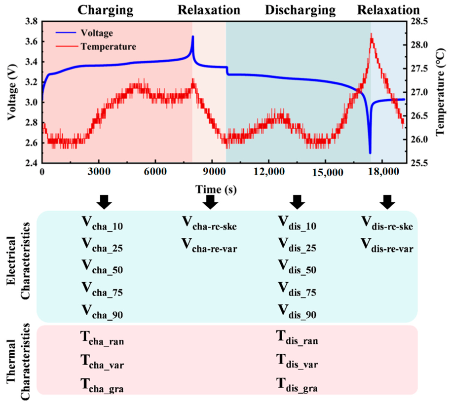
For typical 0.5P large-capacity energy storage batteries, approximately 15,000 data points are generated during each charge and discharge cycle. The tested commercial energy storage batteries are LiFePO₄/graphite large-capacity products provided by the China Electric Power Research Institute (Beijing, China) under a national key R&D project. All batteries were cycled following the GB/T 36276 constant-power (0.5P) charge/discharge protocol with 3.65 V upper cut-off voltage and 2.5 V lower cut-off voltage. Two datasets were established under different ambient temperatures: the 25 °C dataset contains 10 batteries covering five rated capacities (320, 153, 290, 29, and 155 Ah), and the 45 °C dataset includes 12 batteries from four rated capacities (280, 314, 314, and 340 Ah). All samples adopt a graphite anode and LiFePO₄ cathode, consistent with mainstream commercial LFP energy storage batteries. Detailed proprietary internal structural parameters (electrode coating loading, separator material, geometric dimensions, etc.) cannot be fully disclosed by the manufacturer; thus, only public commercial specifications and core electrochemical compositions of all tested batteries are reported. The vast amount of data imposes a significant burden on model training, and an excessive number of features results in the overfitting of the prediction model. In addition, some of the extracted features were redundant or irrelevant. Therefore, prior to model training, it is essential to filter out the health features that are highly correlated with battery aging. For example, Figure 1 illustrates the health features of energy storage batteries tested according to the GB/T 36276-2023 testing standards. Twenty health features were extracted from a complete charge and discharge cycle, including the 10th, 25th, median, 75th, and 90th percentiles of both charging and discharging voltages, range and variance of charging and discharging temperatures, gradient of charging and discharging temperatures, and skewness and variance of the relaxation voltage during charging and discharging. The temperature gradient indicates the rate of temperature change, whereas the skewness of the relaxation voltage reflects the symmetry of the relaxation voltage curve.

The correlation analysis between these 20 features and the SOH is conducted, introducing the Pearson correlation coefficient [27] ${\rho }_{\mathrm{x}\mathrm{y}}$, calculated as follows:

$${\rho }_{\mathrm{xy}}={\displaystyle \frac{{\displaystyle \sum (X-\overline{X})(Y-\overline{Y})}}{\sqrt{{\displaystyle \sum {(X-\overline{X})}^2·}{\displaystyle \sum {(Y-\overline{Y})}^2}}}}$$

(3)

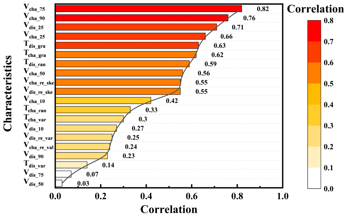
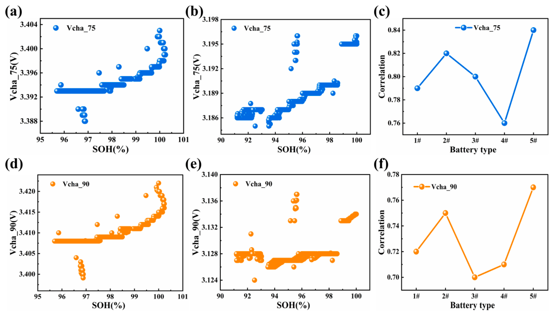
where $\overline{X}$ represents the average value of $X$, and $\overline{Y}$ represents the average value of $Y$. The closer the value of $\left|{\rho }_{\mathrm{x}\mathrm{y}}\right|$ is to 1, the stronger the correlation between the feature and SOH. Figure 2 shows the correlation results for all features with SOH. The feature with the highest correlation was the 75th percentile of the charging voltage, with a correlation coefficient of 0.82, followed by the 90th percentile of the charging voltage with a correlation coefficient of 0.76. Figure 3 illustrates the variation in some aging features with SOH, clearly demonstrating how health features change with SOH. Among the voltage feature parameters, the charging process of the energy storage battery cell is more correlated with the battery’s health status than the discharging process, and better reflects the aging information of the battery. Regarding the temperature parameters, the temperature range during charging and discharging was more strongly correlated with the health status of the battery. In this study, the three health features with the highest correlation were selected: the 75th percentile of the charging voltage, the 90th percentile of the charging voltage, and SOH. The step-like variation in Vcha_75 with SOH shown in Figure 3a,b does not show discrete electrochemical degradation stages. Instead, it results from cycle-wise statistical feature extraction, SOH measurement discretization, and plotting effects, whereas the underlying aging process remains continuous. The selected voltage features still exhibit strong monotonic correlation with SOH, for being suitable for LSTM-based life prediction. Pearson analysis is used only as a second-stage screening tool after mechanism-guided feature definition, while nonlinear degradation dynamics are modeled by the LSTM network. The three selected input features are consistently defined as the 75th percentile of charging voltage, the 90th percentile of charging voltage, and historical SOH. Pearson correlation analysis is employed to screen mechanism-defined candidate features rather than to replace physical feature design. Nonlinear degradation behavior is modeled by the LSTM network.

These two voltage features with the highest correlation coefficients were selected as model inputs. The selection is supported by both empirical data analysis and extensive literature evidence. In the later charging stages, active lithium loss is caused by two mechanisms: lithium-ion intercalation into the negative electrode and SEI (solid electrolyte interphase) layer growth [28]. The selected parameters are found to be consistent with the underlying electrochemical mechanisms. Additionally, lower correlation coefficients are observed in temperature signals compared to voltage signals. For large-capacity energy storage batteries, this discrepancy is potentially attributed to the delayed response between measured surface temperature and internal temperature, resulting in measurement deviations.

2.2. Input Data Processing

Owing to various factors such as the measurement conditions, significant outliers and noise were present in the original data. Appropriate processing methods must be applied to the dataset to address these anomalies and spurious data fragments while preserving the characteristics of the original data. In this study, the method of replacing outliers with the average of the preceding and following values was used for cases where the outliers were minor points after observing the data types. SG filtering was employed for the data that exhibited abnormal jitter segments. SG filter [29] is a mathematical tool used for data smoothing. Its core principle involves fitting the data points within a certain length window using a kth-order polynomial and determining the fitting parameters through the least-squares method, thus achieving data smoothing. The advantage of an SG filter is that it removes noise while preserving the shape and width of the data without altering the overall trend.

The parameter selection of the SG filter had a significant impact on the filtering effect. The window length and order of the polynomial (polyorder, denoted as k) are two key parameters. The window length determines the smoothness of the filter; a larger window length results in a more pronounced smoothing effect. The order of the polynomial affects the accuracy of the fitting, with a higher order leading to a fitting closer to the original data; however, an excessively high order may cause overfitting.

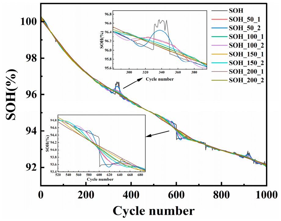
In this study, a full testing cycle of 1000 cycles and a feature data length of 1000 were considered. The window sizes of the SG filter were set to 50, 100, 150, and 200, and the polynomial orders were set to 1 and 2. The SOH data were then subjected to SG filtering, and the results are illustrated in Figure 4.

The filtering process must consider both the degree of smoothing and the similarity of the filtered data to the actual trend. Compared to the original data, the filtered curves were smoother without over-smoothing, which may obscure the true variations in the trend. The optimal combination of parameters was determined to be a window size of 150 and a polynomial order of 1. Window sizes smaller or larger than 150 did not yield satisfactory fitting results. When the polynomial order was set to 2, the filtering results emphasized the local features while neglecting the overall trend.

Gradient descent optimization algorithms rely on neural networks to update the parameters. If the range of feature values varies significantly, the update direction of gradient descent may become unstable, leading to slow training processes or convergence to local optima. If excessively large or small input values are provided to activation functions (such as Sigmoid or Tanh), output values may saturate, leading to vanishing gradients and preventing further learning by the model. Therefore, normalization, which scales all feature values to a consistent range (such as [0, 1] or [−1, 1]), results in a more uniform gradient descent update direction, thereby accelerating the convergence speed of the model and enhancing its stability. In this study, the maximum-minimum normalization method was used to normalize the input data, and the calculation formula is as follows:

$${\mathrm{x}}^{\prime }={\displaystyle \frac{x-x_{\min }}{x_{\max }-x_{\min }}}$$

(4)

After maximum–minimum normalization, the feature data were mapped to the [0, 1] interval.

2.3. Sliding Time Window Method

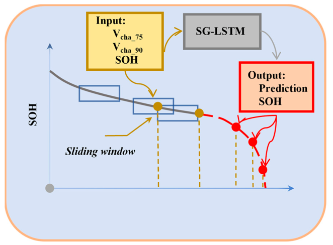
In time-series analysis, models that can capture patterns and trends evolving over time are necessitated by the dynamic nature of the data. Temporal dependencies present in the data are often overlooked by traditional static analysis methods. In contrast, this issue is addressed by sliding time window methods through the construction of training samples that maintain temporal continuity. In this study, deterministic time-series data is selected as the feature of maximum discharge energy, in which nonlinear changes in the charging and discharging energy of batteries are exhibited as the number of cycles increases. To enhance the understanding and predictive capabilities of the model regarding time-series data, a sliding time window method is proposed for the construction of training samples. A time window is defined as a fixed-length continuous period that is used to capture local dynamic characteristics within a time series. The sliding of the time window is accomplished by moving forward along the time axis with a specified stride. The data within each time window serves as a training sample, ensuring temporal continuity among samples. An adaptive window size approach is employed for the selection of time windows, allowing the window size to be dynamically adjusted based on the intrinsic features of the data to better accommodate different time-series characteristics. The principle of the sliding time window method is illustrated in Figure 5. The advantage lies in the fact that during training, vector windows are fully input into the model in the form of x–y for comprehensive training. In the prediction phase, only the first vector derived from early aging data needs to be input to predict subsequent sequence changes, and the results are then fed back into the input vector for continuous iteration, thereby achieving the remaining life prediction of the battery. The issue of significant model errors caused by insufficient utilization of limited experimental data is effectively addressed by the sliding window method.

The principle of time window sliding for predicting the RUL of the battery is as follows: Assume that the time window size is $N_{\mathrm{window}}$, each time window is a training sample, the length of a single battery data is $N_i$, and the inputs are $(V_{\mathrm{cha}\_75\_1},V_{\mathrm{cha}\_90\_1},{\mathrm{SOH}}_1)$, $(V_{\mathrm{cha}\_75\_2},V_{\mathrm{cha}\_90\_2},{\mathrm{SOH}}_2)$, …, and $(V_{\mathrm{cha}\_75\_N_{\mathrm{window}}},V_{\mathrm{cha}\_90\_N_{\mathrm{window}}},{\mathrm{SOH}}_{N_{\mathrm{window}}})$. After model training to obtain the predicted value $(V_{\mathrm{cha}\_75\_N_{\mathrm{window}+1}},V_{\mathrm{cha}\_90\_N_{\mathrm{window}+1}},{\mathrm{SOH}}_{N_{\mathrm{window}+1}})$, add the predicted value $(V_{\mathrm{cha}\_75\_N_{\mathrm{window}+1}},V_{\mathrm{cha}\_90\_N_{\mathrm{window}+1}},{\mathrm{SOH}}_{N_{\mathrm{window}+1}})$ to the input, slide the time window one step forward, and then use $(V_{\mathrm{cha}\_75\_2},V_{\mathrm{cha}\_\mathrm{9o}\_2},{\mathrm{SOH}}_2)$, $(V_{\mathrm{cha}\_75\_3},V_{\mathrm{cha}\_90\_3},{\mathrm{SOH}}_3)$, …, and $(V_{\mathrm{cha}\_75\_N_{\mathrm{window}+1}},V_{\mathrm{cha}\_90\_N_{\mathrm{window}+1}},{\mathrm{SOH}}_{N_{\mathrm{window}+1}})$ as the input, model output $(V_{\mathrm{cha}\_75\_N_{\mathrm{window}+2}},V_{\mathrm{cha}\_90\_N_{\mathrm{window}+2}},{\mathrm{SOH}}_{N_{\mathrm{window}+2}})$, etc., in a loop until the prediction of ${\mathrm{SOH}}_{N_i}$. When predicting that the state of the battery is less than 80% after a certain number of loops, we consider that the battery has reached its end of life and then substitute the predicted starting point and the number of loops into formula (2) to obtain the predicted RUL.

For a battery with a data sequence length N_i, when the time window is N_window, the number of samples that the battery can provide is N_i − N_window. Therefore, the total number of samples was $\mathrm{M}={\displaystyle \sum _1^m(N_i-N_{\mathrm{window}})}$, where i is the length of the feature data sequence for the mth battery. In this study, the impact of the time window size on the model accuracy was investigated by setting the time window sizes to 10, 50, 100, 150, 200, 250, and 300.

The complete step-by-step logic of the sliding window algorithm is shown in detail in Section 3.2. Set the total length of the feature sequence for a single battery as L, and the window size is set to w = 150.

Training Stage: Each sample takes the continuous cycle interval [t – w + 1, t] as input, with the state of health at cycle t (or the subsequent time step) as the label. The window slides forward by one cycle each time, generating L – w + 1 samples for each battery.

Prediction stage: starting from the first window formed by measured cycles, the model predicts the next SOH. The window then slides forward one cycle at a time. When measured data are unavailable, the predicted SOH is appended to the input sequence for recursive prediction.

3. Construction of Data-Driven Model

3.1. LSTM Neural Network

LSTM networks were utilized in this study to develop a prediction model for life prediction. The parameters for each layer, along with the model hyperparameters, are listed in

Table 1. The number of nodes in the LSTM model settings.

Network Layer	Parameters
First LSTM layer	64, 128, 256
Second LSTM layer	64, 128, 256
Fully Connected layer	32, 64, 128
Dropout layer	0.01~0.10
Learning rate	0.0001, 0.0005, 0.001

.

The performance comparison between automatic hyperparameter optimization (autotuning) and manual tuning methods is investigated by N. Shawki et al. [30]. The best combination of values listed in the table is identified to optimize the model’s node count, guided by empirical experience. The established prediction model is illustrated in Figure 6.

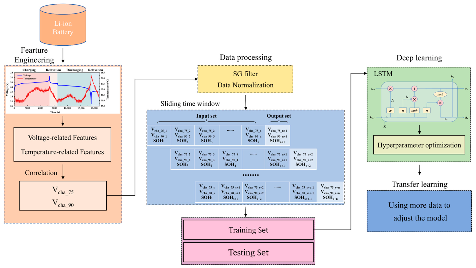
The proposed model can be divided into three stages: data preprocessing, feature extraction and selection, LSTM estimation, and model validation. First, data preprocessing is performed to remove outliers and noise from the raw measurement data, and health features that are highly correlated with SOH are extracted from the battery’s charge–discharge curves to describe its aging condition. Subsequently, the model was utilized to predict the SOH of the battery, and its effectiveness was validated by comparison with other machine learning methods.

3.2. Transfer Learning

When addressing various types of energy storage batteries, a static model struggles to predict the aging differences arising from the diverse characteristics of these batteries. A transfer learning module was introduced to improve the generalization capability of the model. The knowledge and experience gained by the existing model in the source domain (the battery type targeted by the base model) are utilized by this module to swiftly adapt to the prediction tasks in the target domain (new battery types). The substantial data and computational resources required to retrain the model are minimized for new battery types, thereby enhancing the prediction accuracy and adaptability across different battery models. For the aging data of the new energy storage battery types, transfer learning was performed using data from the 151st to the 300th cycle; specifically, certain hyperparameters of the base model were initially frozen to preserve its general feature extraction capabilities and fundamental temporal relationship capture abilities acquired in the source domain, and the unfrozen components of the model were retrained using data from the 151st to the 300th cycle of the new battery type, adjusting these parameters to align with the characteristics of the new battery. In this study, the I-LSTM layer remains frozen, whereas the weights and biases of certain units in the II-LSTM network are fine-tuned. This enables the model to learn the unique features and aging patterns of the new battery type more effectively.

3.3. Evaluation Indicators of the Prediction Model

The RMSE and mean absolute error (MAE) were chosen as evaluation metrics, and both positive and negative errors were regarded as prediction errors. Therefore, MAE was selected to assess the overall bias of the prediction model. In addition, the dispersion of the predicted values is a significant consideration. RMSE is chosen as a supplementary evaluation metric, and the combination of both metrics offers a comprehensive assessment of the model. The formulas for RMSE and MAE are presented below:

$$\mathrm{MAE}={\displaystyle \frac{1}{N}}{\displaystyle \sum _{i-1}^N\left|y_i-{\widehat{y}}_i\right|}$$

(5)

$$\mathrm{RMSE}=\sqrt{{\displaystyle \frac{1}{N}}{\displaystyle \sum _{i=1}^n{(y_i-{\widehat{y}}_i)}^2}}$$

(6)

The true value is $y_i$, the estimated value is ${\widehat{y}}_i$, and N is the sample size.

4. RUL Prediction and Transfer Learning

To assess the feasibility of the proposed life prediction method, aging tests were performed on large-capacity energy storage batteries across various models and temperatures.

4.1. Analysis of RUL Prediction

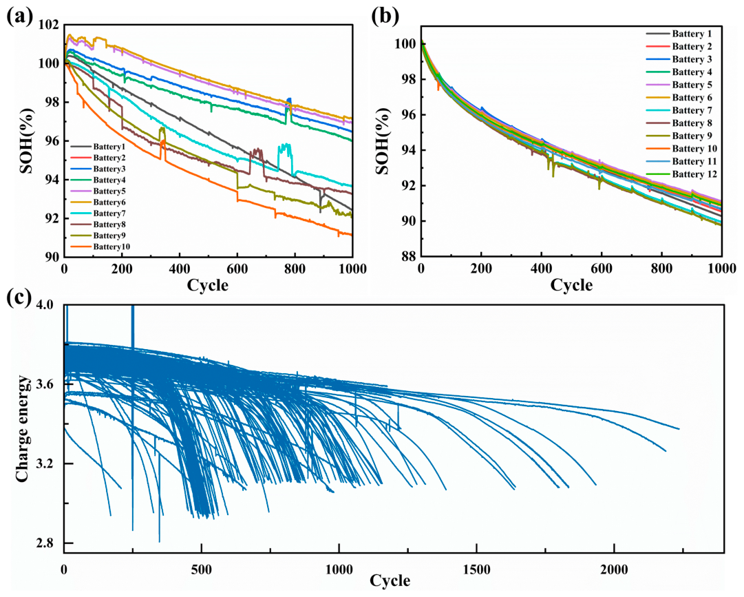
Five types of large-capacity energy storage batteries, totaling 10 units, were selected to perform aging tests and create an aging dataset. The rated capacities of the batteries were 320 Ah, 153 Ah, 290 Ah, 29 Ah, and 155 Ah. In the charge–discharge tests, in accordance with the testing requirements of the Chinese national standard GB/T 36276-2023, the batteries were charged at the rated power to 3.65 V and discharged to 2.5 V at a constant power of 25 °C. For each charge–discharge cycle, aging data, including voltage, current, temperature, and charge–discharge energy, were recorded. The tests were terminated after 1000 cycles. The relationship between the health state of the energy storage batteries and the number of cycles is illustrated in Figure 7a.

Batteries 1–8 were used as the training set, and Batteries 9 and 10 were designated as the validation set. Following previously described methods, the aging feature parameters were extracted for each cycle, and outlier and SG filtering techniques were applied. Subsequently, training vectors were generated, and the life prediction model was trained using the sliding window method. Hyperparameter optimization was conducted for the model based on the ranges listed in Table 1. An optimal set of hyperparameters for this batch of batteries at 25 °C is identified as [256, 256, 64, 0.05, 0.0005]. This indicated that the number of nodes in the first LSTM hidden layer was 256, the number of nodes in the second LSTM hidden layer was 256, the number of nodes in the FCL was 64, and the learning rate was 0.0005. The SOH feature included in the input sequence refers to historical measured SOH values within the sliding window SOH. Therefore, information leakage is avoided during training. In practical deployment, historical SOH can be obtained from measured capacity or BMS estimates, while recursive prediction may gradually use SOH values predicted when measured data are unavailable.

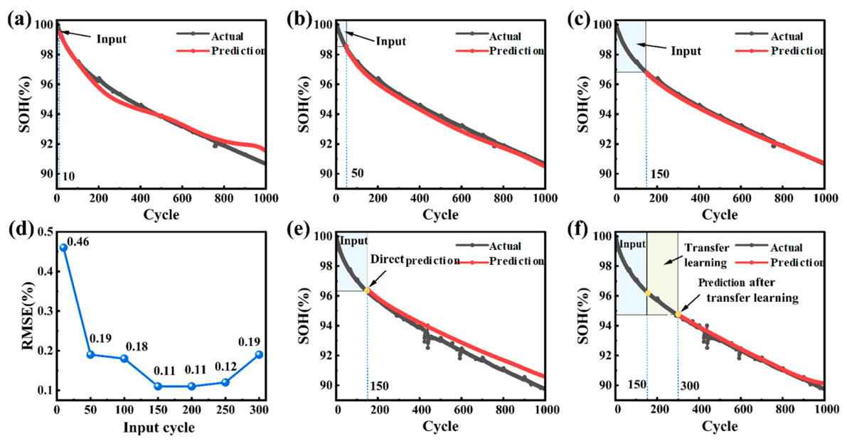
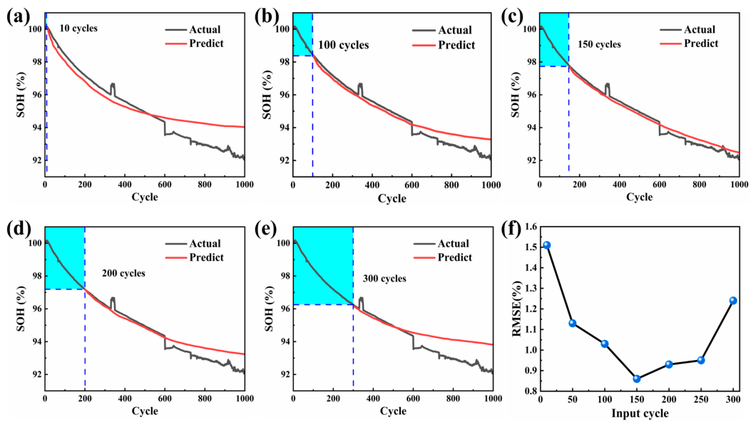
Initially, the effect of varying the input vector lengths (number of cycles) on the accuracy of the life prediction model was examined, and the results are presented in Figure 8. When only 10 cycles of aging data were utilized as the model input, a significant discrepancy was observed between the predicted SOH and the actual SOH (Figure 8a), with an average RMSE of 1.51% in the validation set. When the input window was expanded to 100 cycles (Figure 8b), the prediction accuracy improved marginally compared to the use of 50 cycles as the input, with the RMSE decreasing to 1.03%. When 150 cycles were utilized as the model input, the predicted curve closely matched the actual curve (Figure 8c), and the prediction accuracy increased significantly, with the RMSE decreasing to 0.86%. When the input window was expanded to 200 cycles (Figure 8d), the RMSE values was 0.93%, indicating a minimal difference compared with the use of 150 cycles. However, when the input window was expanded to 300 cycles, the RMSE unexpectedly increased to 1.24% (Figure 8e), which may be attributed to overfitting resulting from the excessive input length. Furthermore, as the input length increases, the number of training samples generated by the sliding window method decreases, which may also contribute to the increase in the prediction error despite the larger input window.

Smaller prediction errors signify higher prediction accuracy, whereas shorter input data lengths correspond to reduced actual battery testing and evaluation times. Considering both factors, 150 data cycles were selected as the optimal input vector length for the model. Second, to validate the superiority of LSTM neural networks, the performances of other conventional machine learning methods were compared in predicting the lifespan of large-capacity energy storage batteries, including support vector machines (SVMs), convolutional neural networks (CNNs), recurrent neural networks (RNNs), and Transformer. Because these methods have been extensively discussed in numerous papers, detailed information on them can be found in the literature [31,32,33,34]. All benchmark models adopt the same features of the preprocessing workflow, sliding-window settings, and dataset partition. Hyperparameters of the LSTM model are optimized within the ranges given in

Table 2. Structural configurations, training hyperparameters and prediction errors of all comparative models.

Model	Optimal Structure & Hyperparameters	Optimizer	Batch	Epoch	RMSE(%)
LSTM (This work)	LSTM (256→256) + FC (64), Dropout = 0.05, lr = 0.0005	Adam	32	300	0.86
RNN	RNN (256→256) + FC (64), Dropout = 0.05, lr = 0.0005	Adam	32	300	1.42
CNN	Conv1d (64, k = 5) + Conv1d (128, k = 3) + FC (64), Dropout = 0.05, lr = 0.0005	Adam	32	300	1.28
Transformer	d_model = 128, heads = 4, layers = 2, FFN = 256, Dropout = 0.05, lr = 0.0005	Adam	32	300	1.15
SVM	Flattened 450-dimensional input, RBF kernel, C = 10, γ = 0.01, ε = 0.05	—	—	—	1.56

. The benchmark models are tuned under the same input conditions to ensure comparison fairness.

Table 3. RMSE of RUL prediction with different machine learning methods.

Machine Learning Methods	SVM	CNN	RNN	Transformer	Proposed Methods (LSTM)
RMSE/%	1.37	1.32	1.1	1.15	0.86

presents the average RMSE of the life prediction models derived from the aforementioned machine learning methods applied to the same validation set. Compared to other machine learning methods, LSTM exhibits the lowest prediction error, further validating its superiority in addressing time-series data prediction challenges, which is attributed to its unique gating design of memory cells and forget gates.

4.2. Analysis of Transfer Learning Results

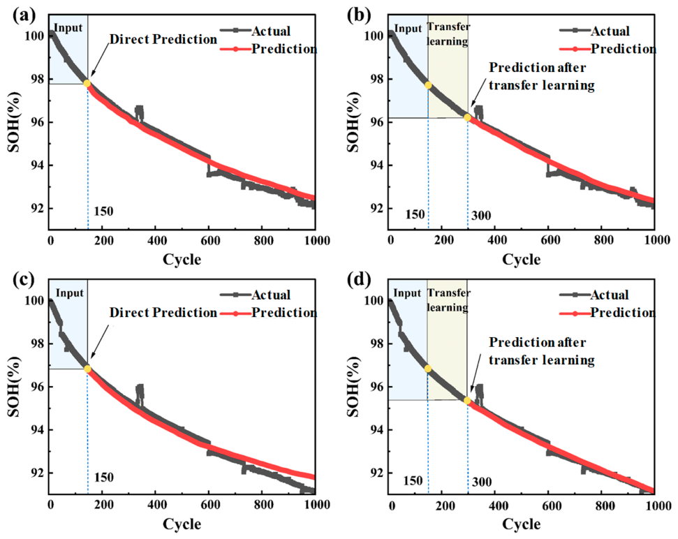
To assess the enhancements provided by transfer learning in the life prediction of energy storage batteries, the results of direct prediction were compared with those obtained after transfer learning using the basic life prediction model for new types of energy storage batteries, as shown in Figure 9. Figure 9a,c presents the lifetime prediction results when the model is directly applied to new types of energy storage batteries that are not included in the dataset without utilizing transfer learning. The life prediction deviation was substantial, with an RMSE of 0.86% over the entire 1000-cycle testing period. Figure 9b,d shows the life prediction results following transfer learning. Aging data from the 151st to 300th cycles were utilized to adjust the basic model in accordance with the method described in Section 3.2. Following transfer learning, the predicted health status of the energy storage battery was closely aligned with the actual health status, with the prediction error RMSE decreasing to 0.18%. These results indicate that transfer learning can effectively rectify deviations in life predictions for new types of energy storage batteries. In summary, when early battery data (300 cycles) are available, the combination of an LSTM-based life prediction model with transfer learning can yield accurate predictions of the remaining lifespan of energy storage batteries.

4.3. Verify the Robustness of the Model

To further validate the effectiveness of the model, the method proposed in this study for extracting health features from charge–discharge curves was applied to two additional battery datasets. The first dataset comprised aging data from 12 large-capacity energy storage batteries across four different models with rated capacities of 280 Ah, 314 Ah, 314 Ah, and 340 Ah. In the charge–discharge tests, in accordance with the testing requirements of the Chinese national standard GB/T 36276-2023, the batteries were charged at the rated power to 3.65 V and discharged to 2.5 V at a constant power at 45 °C. Aging data, including voltage, current, temperature, and charge–discharge energy, were recorded for each charge–discharge cycle, and the tests were terminated after 1000 cycles. Compared to the testing conditions of the previous battery set, the only change was an increase in testing temperature from 25 °C to 45 °C, while the other conditions remained unchanged. The relationship between the health state of the energy storage batteries and the number of cycles for this battery set is illustrated in Figure 7b.

The proposed method was applied to this dataset to extract the aging feature parameters for each battery cycle, manage outliers, and conduct SG filtering. The training vectors were subsequently generated, and the life prediction model was trained using the sliding window method. Batteries 1–9 were used as the training set, whereas batteries 10–12 were used as the validation set. The first 300 cycles of data from the validation set batteries were used for transfer learning to adjust the model. The prediction and transfer learning results are shown in Figure 10. The prediction results demonstrated that the feature extraction method and prediction model proposed in this study yielded favorable outcomes, accurately predicting the SOH of batteries throughout the entire national standard testing cycle in China (1000 cycles). Detailed error statistics are presented in Figure 10d, indicating that the MAE for direct predictions was less than 0.10%, and the RMSE for batteries 10–12 was below 0.15%. Following transfer learning, the RMSE for all three batteries decreased significantly. The comparative prediction results between direct forecasting and transfer learning approaches for Battery No. 10 are illustrated in Figure 10e,f. A reduction in RMSE from 0.50% to 0.10% is achieved through the implementation of transfer learning. In the data for battery no. 12, some cycles exhibited abnormal capacities; however, the model proposed in this study delivered accurate predictions for such scenarios, demonstrating the high reliability and accuracy of the proposed model and feature selection techniques.

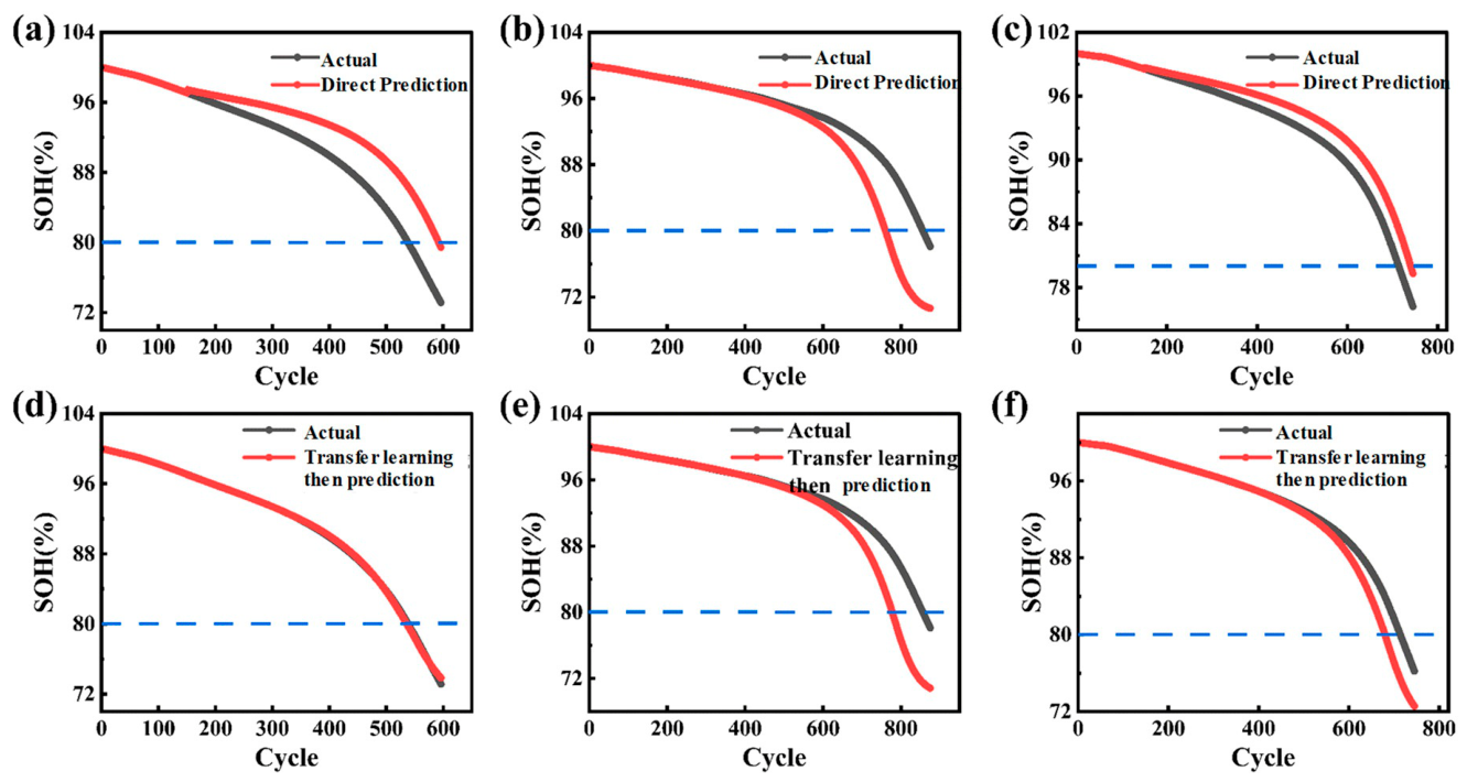
The second dataset was released by MIT [35]. This dataset comprised 124 commercial LiFePO₄/graphite batteries that were cycled under different fast-charging conditions but with the same discharge conditions (4C constant current). Fast-charging strategies include multistage constant current (MCC) charging and constant voltage (CV) charging. The format of MCC is “C1 (Q1)-C2,” where C1 and C2 are the current rates for the first and second steps, respectively, and Q1 is the SOC point at which the current is switched. The second step ended at 80% SOC, after which the battery was charged with a 1C current under constant-current and constant-voltage conditions. All batteries were cycled in an indoor environment at an ambient temperature of 30 °C until their capacity dropped below 80% of the nominal value. Compared with the previous two large-capacity energy storage battery datasets, the nominal capacity of this battery is only 1.1 Ah, with the upper and lower voltage limits being 3.6 V and 2.0 V, respectively. The lifespans of these 124 batteries varied widely, ranging from 400 to 2000 cycles. The method proposed in this study was also applied to this dataset by extracting aging features, processing the data, creating training vectors according to the sliding window method, and then inputting them into the model for prediction. Five batteries with lifespans of approximately 500 cycles and five batteries with lifespans of approximately 1200 cycles were randomly selected for validation, using the remaining batteries as the training set. Comparative experiments with varying input data lengths were conducted, and a minimal prediction error was observed at an input window of 150 time steps. No significant changes in prediction error are observed when the input window exceeds 150 time steps. Comparative experiments were also conducted with different lengths of input data. It was found that the prediction error was the lowest when the input window was 150 and remained almost unchanged as the input window continued to increase. Transfer learning was performed to refine the model using the first 300 cycles of data from the validation set of the batteries. Compared to the test conditions in the Chinese national standard GB/T 36276-2023, the MIT dataset test conditions differed in the charging mode, upper and lower voltage limits, and test temperature. The prediction and transfer learning results are shown in Figure 11. The prediction results for four batteries with varying lifespans are presented in Figure 11a–c, where the initial 150 cycles are utilized as input data. Transfer learning outcomes for the identical battery set are illustrated in Figure 11d–f, with cycles 151–300 serving as the input data. The prediction results indicate that the feature extraction method and prediction model proposed in this study have shown good predictive performance on the MIT open-source battery dataset, achieving accurate predictions of the full lifecycle of batteries of different lengths. The model can accurately predict the lifespan inflection points for batteries with lifespans of approximately 500 and 1200 cycles. The average prediction error RMSE for the batteries in the validation set being 4.3%. After transfer learning, the prediction error further decreased to 3.1%. Compared with the large-capacity datasets obtained under GB/T 36276, the MIT dataset differs substantially in nominal capacity, voltage limits, charging protocols, test temperature, and lifespan distribution. The higher RMSE (4.3%) on the MIT dataset should therefore be interpreted as a cross-domain validation result rather than a direct comparison with the in-domain performance on large-capacity batteries (<1%). In addition, the recursive prediction framework causes error accumulation over long horizons, which further affects the overall RMSE. Transfer learning reduces the MIT validation RMSE to 3.1%, indicating that the method remains applicable under heterogeneous conditions.

However, as shown in Figure 11, as the prediction window continued to slide backward, the prediction error gradually increased. This is because the data used as input later are all predicted based on early battery data, and the prediction error continues to accumulate as the prediction window slides backward, which is another drawback of this model. As shown in Figure 11b, a noticeable deviation between the predicted and actual SOH values appears around 600–800 cycles near the 80% SOH threshold. This is mainly caused by error accumulation in the recursive sliding-window prediction and the accelerated nonlinear degradation near end-of-life. The present method has inherent limitations in long-horizon autoregressive prediction, especially for batteries with fast-charging protocols and diverse lifespans. Future improvements may include online updating with measured data, transfer learning, hybrid physics-informed correction, and periodic recalibration near the end-of-life region. The increasing prediction error on the MIT dataset is mainly caused by error accumulation in recursive sliding-window prediction, rather than by insufficient LSTM alone. For ultra-long lifespan batteries, the baseline model can be combined with transfer learning and periodic recalibration using newly measured data to maintain long-term prediction accuracy.

The method and prediction model proposed in this study can not only accurately predict the SOH of large-capacity energy storage batteries within the Chinese national testing and evaluation cycle of GB/T 36276-2023 (1000 cycles) but also precisely predict the remaining full life cycle of small-capacity batteries. Exceptional performance was demonstrated by the model across datasets comprising batteries with different cycling test conditions, testing temperatures, and various models. Through data analysis, three key aging parameters, namely, the 75th percentile of the charging voltage, the 90th percentile of the charging voltage, and SOH, were selected from 20 aging features of the charge–discharge curve, highlighting the high reliability of the proposed method. Additionally, a transfer learning module was developed to refine the model using the first 300 cycles of data from new battery models, effectively improving the prediction accuracy of the model for new battery types and demonstrating the practical generalization ability of the prediction model. This study provides a practical technical method for actual energy storage battery testing and evaluation.

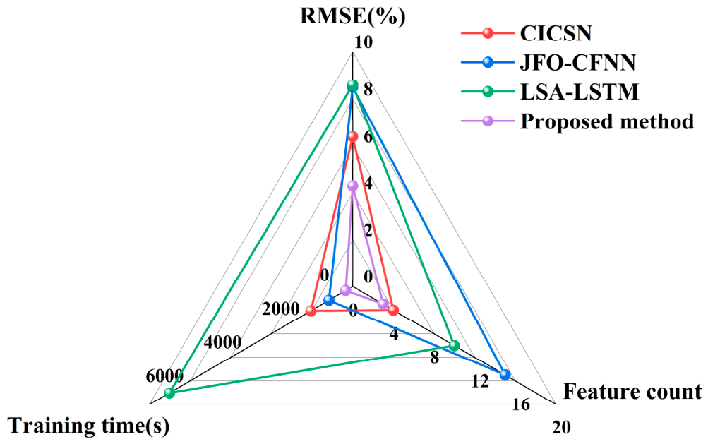
A comprehensive performance evaluation of the proposed model is conducted through comparison with several state-of-the-art models reported in the literature [19,36,37]. The evaluation is performed based on three critical performance metrics: RMSE, feature count, and training time. Cross-dimensional comparison is facilitated through radar chart visualization (Figure 12). A balanced performance profile of the proposed model is illustrated by the radar chart analysis. The proposed model’s superior predictive capability is demonstrated by achieving a lower RMSE compared to benchmark models. An RMSE reduction of 2% is achieved (4.3%) relative to the benchmark models’ mean RMSE. The proposed model achieves comparable performance with only three features, while benchmark models require more extensive feature sets. Training efficiency is significantly improved, with a reduced training time of 240 s compared to benchmark models (820 s–6300 s). Superior performance in accuracy, feature efficiency, and computational economy is revealed through the radar chart analysis. The model’s robustness and practical applicability for real-world scenarios are validated by the comprehensive performance metrics.

The training time recorded in this work corresponds to offline GPU workstation training rather than embedded on-board BMS operation. The present efficiency assessment focuses on algorithm-level offline performance, without fully quantifying edge-side overhead, including real-time inference latency, runtime memory footprint, data buffering cost, and parameter updating overhead brought by transfer learning. Comprehensive hardware deployment tests and quantitative measurement of embedded computational cost on real BMS chips will be conducted in follow-up research.

To assess model robustness, Gaussian noise with amplitudes of 1%, 5%, 10%, and 15% was added to the training-set input features. The validation RMSE of the proposed LSTM model under different noise levels is reported in

Table 4. Average validation RMSE under different training-set noise levels.

Noise Level of the Training Set	Average RMSE of Validation Set (%)
0% (no noise)	0.86
1%	0.94
5%	1.12
10%	1.28
15%	1.51

. The results show that the model maintains acceptable prediction accuracy under moderate measurement noise. When the noise amplitude reaches 15%, the average validation RMSE only rises to 1.51%, which is still within the error tolerance range for industrial energy storage battery aging evaluation. This stable performance demonstrates the strong anti-interference capacity of the mechanism–data co-driven framework, as the prior electrochemical feature screening effectively suppresses the interference of random measurement noise. Each noise-level experiment was repeated 10 times by random network initialization. The RMSE values listed in Table 4 correspond to the average results of repeated tests, which eliminates accidental bias from a single training run and improves the statistical reliability of the validation results.

5. Conclusions and Discussions

In this study, a method for predicting the lifespan of large-capacity energy storage batteries was proposed based on early battery aging data and transfer learning. This method was validated on other battery datasets, effectively addressing the challenges of reliability and generalizability encountered by current battery life prediction models in practical applications. First, 20 voltage- and temperature-related features were extracted from the charge–discharge curves. The three features with the highest correlation with the SOH were selected as the input features for the model. Subsequently, outliers were addressed by replacing them with mean values. SG filtering was proposed to eliminate the noise caused by measurements, with the optimal set of parameters determined through observation. A sliding window method was then introduced to create training samples, and a lifespan prediction model for energy storage batteries based on LSTM neural networks was developed. Finally, a transfer learning module was created to refine the model using the first 300 cycles of data from the new battery models, thereby enhancing prediction accuracy. The effectiveness of the feature extraction and prediction model was validated using a dataset of energy storage batteries tested in accordance with the Chinese national standard GB/T 36276-2023. The prediction results demonstrated very small overall errors, essentially aligning with the true values. Furthermore, the proposed feature extraction method and prediction model were validated using the MIT dataset, which yielded similarly low prediction errors (RMSE). This demonstrated the high reliability and robustness of the proposed model. Compared with other classic machine learning methods, the proposed LSTM model achieved the highest accuracy, with errors significantly lower than those of the alternative methods. This demonstrates its substantial advantages and reliability in predicting the lifespan of energy storage batteries. This method can decrease the number of battery test cycles and experimental time required for practical battery testing scenarios.

The primary contributions of this work are summarized as follows:

(1) It is demonstrated that the method of extracting and selecting features highly correlated with the SOH from battery charge–discharge curves effectively reduces the amount of input data while maintaining a high level of model prediction accuracy.

(2) A prediction model for the remaining lifespan of batteries was developed based on the LSTM network. The influence of input length on model accuracy was investigated. Considering both prediction accuracy and input data length, an input length of 150 cycles was ultimately chosen. This significantly decreased the experimental time required for practical battery testing and evaluation.

(3) A transfer learning module was created based on the life prediction model. For new types of energy storage batteries not included in the training data, the model was fine-tuned and optimized for adaptability using data from the 151st to 300th cycles. For the energy storage battery set tested in accordance with the Chinese national standard GB/T 36276-2023 at 25 °C (comprising five models and 10 batteries), the prediction error is reduced from 0.86% to 0.18%. This facilitates the precise prediction of the battery lifespan for any model of a large-capacity energy storage battery based on early aging data from the first 300 cycles throughout the complete testing cycle of the Chinese national standard.

(4) The methods and prediction models proposed in this study have wide-ranging application prospects in the field of energy storage battery production and testing. On the one hand, this study can significantly decrease the time required for R&D testing of energy storage batteries. However, it addresses the gap in cycle performance evaluation during random inspections of energy storage power station batteries, providing technical support for quality control and the efficient development of the battery energy storage industry.

Battery cycle life prediction is significantly affected by internal temperature variations and thermal delays. By integrating an optimized internal temperature estimation architecture with adaptive thermal feature extraction, the prediction performance degradation delays can be further reduced, thereby improving the long-term robustness and accuracy of the LSTM-based life prediction system. This work focuses on standardized constant-power aging tests for commercial storage batteries. Future work will draw on state-of-the-art electrothermal coupling models for lithium batteries to achieve more accurate internal battery temperature and refine thermal feature extraction with the validation under highly dynamic frequency regulation or peak-shaving grid profiles.

References

1. Tang, X.; Zou, C.; Wik, T.; Yao, K.; Xia, Y.; Wang, Y.; Yang, D.; Gao, F. Run-to-Run Control for Active Balancing of Lithium Iron Phosphate Battery Packs. IEEE Trans. Power Electron. 2020, 35, 1499–1512. [Google Scholar] [CrossRef]
2. Wu, Y.; Li, W.; Wang, Y.; Zhang, K. Remaining Useful Life Prediction of Lithium-Ion Batteries Using Neural Network and Bat-Based Particle Filter. IEEE Access 2019, 7, 54843–54854. [Google Scholar] [CrossRef]
3. Nair, P.; Vakharia, V.; Borade, H.; Shah, M.; Wankhede, V. Predicting Li-Ion Battery Remaining Useful Life: An XDFM-Driven Approach with Explainable AI. Energies 2023, 16, 5725. [Google Scholar] [CrossRef]
4. Lee, G.; Kim, J.; Lee, C. State-of-health estimation of Li-ion batteries in the early phases of qualification tests: An interpretable machine learning approach. Expert Syst. Appl. 2022, 197, 12. [Google Scholar] [CrossRef]
5. Tian, J.; Xiong, R.; Shen, W.; Sun, F. Electrode ageing estimation and open circuit voltage reconstruction for lithium ion batteries. Energy Storage Mater. 2021, 37, 283–295. [Google Scholar] [CrossRef]
6. Si, X.; Li, T.; Zhang, Q.; Hu, C. Prognostics for Linear Stochastic Degrading Systems with Survival Measurements. IEEE Trans. Ind. Electron. 2020, 67, 3202–3215. [Google Scholar] [CrossRef]
7. Rauf, H.; Khalid, M.; Arshad, N. Machine learning in state of health and remaining useful life estimation: Theoretical and technological development in battery degradation modelling. Renew. Sustain. Energy Rev. 2022, 156, 27. [Google Scholar] [CrossRef]
8. Dai, H.; Jiang, B.; Hu, X.; Lin, X.; Wei, X.; Pecht, M. Advanced battery management strategies for a sustainable energy future: Multilayer design concepts and research trends. Renew. Sustain. Energy Rev. 2021, 138, 110480. [Google Scholar] [CrossRef]
9. Lipu, M.S.H.; Hannan, M.A.; Hussain, A.; Hoque, M.M.; Ker, P.J.; Saad, M.H.M.; Ayob, A. A review of state of health and remaining useful life estimation methods for lithium-ion battery in electric vehicles: Challenges and recommendations. J. Clean. Prod. 2018, 205, 115–133. [Google Scholar] [CrossRef]
10. Liu, Y.; Sun, G.; Liu, X. Remaining useful life prediction of lithium-ion batteries based on peak interval features and deep learning. J. Energy Storage 2023, 73, 12. [Google Scholar] [CrossRef]
11. Tian, J.; Liu, X.; Li, S.; Wei, Z.; Zhang, X.; Xiao, G.; Wang, P. Lithium-ion battery health estimation with real-world data for electric vehicles. Energy 2023, 270, 12. [Google Scholar] [CrossRef]
12. Waag, W.; Fleischer, C.; Sauer, D.U. Critical review of the methods for monitoring of lithium-ion batteries in electric and hybrid vehicles. J. Power Sources 2014, 258, 321–339. [Google Scholar] [CrossRef]
13. GB/T 36276-2023; Lithium Ion Battery for Electrical Energy Storage. China Standards Press: Beijing, China, 2023.
14. Wang, F.K.; Mamo, T. A hybrid model based on support vector regression and differential evolution for remaining useful lifetime prediction of lithium-ion batteries. J. Power Sources 2018, 401, 49–54. [Google Scholar] [CrossRef]
15. Krupp, A.; Beckmann, R.; Diekmann, T.; Liebig, G.; Freg, E.; Schuldt, F.; Agert, C. Semi-empirical cyclic aging model for stationary storages based on graphite anode aging mechanisms. J. Power Sources 2023, 561, 13. [Google Scholar] [CrossRef]
16. Zhang, Y.; Xiong, R.; He, H.; Pecht, M.G. Long Short-Term Memory Recurrent Neural Network for Remaining Useful Life Prediction of Lithium-Ion Batteries. IEEE Trans. Veh. Technol. 2018, 67, 5695–5705. [Google Scholar] [CrossRef]
17. Hochreiter, S. Long Short-Term Memory; Neural Computation MIT-Press: Cambridge, MA, USA, 1997. [Google Scholar]
18. Sherstinsky, A. Fundamentals of Recurrent Neural Network (RNN) and Long Short-Term Memory (LSTM) network. Phys. D-Nonlinear Phenom. 2020, 404, 28. [Google Scholar] [CrossRef]
19. Xie, P.; Pang, X.; Wang, C.; Yang, W.; Zou, H.; Zhao, W.; Chen, S.; Liu, Z. A sequence to sequence prediction model for remaining useful life of lithium-ion batteries with Bayesian optimisation process visualization. J. Energy Storage 2024, 87, 12. [Google Scholar] [CrossRef]
20. Reza, M.S.; Hannan, M.A.; Mansor, M.; Ker, P.J.; Rahman, S.A.; Jang, G.; Mahlia, T.M.I. Towards enhanced remaining useful life prediction of lithium-ion batteries with uncertainty using optimized deep learning algorithm. J. Energy Storage 2024, 98, 18. [Google Scholar] [CrossRef]
21. Li, X.; Yu, H.; Wang, J.; Xia, Y.; Zheng, H.; Song, H. Prediction of state-of-health of lithium-ion battery based on CEEMDAN-SG-LSTM combined model. Mater. Today Sustain. 2024, 28, 25. [Google Scholar] [CrossRef]
22. Xing, X.Q.; Yan, T.T.; Xia, M. Early prediction of battery life using an interpretable health indicator with evolutionary computing. Reliab. Eng. Syst. Saf. 2025, 260, 110980. [Google Scholar] [CrossRef]
23. Hou, G.L.; Zhang, F.; Huang, C.Z.; Huang, T. Joint prediction of SOH and RUL for Lithium-ion batteries by an enhanced Transformer model with physical information constraints. Energy 2025, 336, 138435. [Google Scholar] [CrossRef]
24. Wang, F.J.; Zhai, Z.; Zhao, Z.B.; Di, Y.; Chen, X.F. Physics-informed neural network forlithium ion battery degradation stable modeling and prognosis. Nat. Commun. 2024, 15, 4332. [Google Scholar] [CrossRef] [PubMed]
25. Afshari, S.S.; Cui, S.; Xu, X.; Liang, X. Remaining Useful Life Early Prediction of Batteries Based on the Differential Voltage and Differential Capacity Curves. IEEE Trans. Instrum. Meas. 2022, 71, 9. [Google Scholar] [CrossRef]
26. Semeraro, C.; Caggiano, M.; Olabi, A.G.; Dassisti, M. Battery monitoring and prognostics optimization techniques: Challenges and opportunities. Energy 2022, 255, 124538. [Google Scholar] [CrossRef]
27. Pepe, S.; Ciucci, F. Long-range battery state-of-health and end-of-life prediction with neural networks and feature engineering. Appl. Energy 2023, 350, 11. [Google Scholar] [CrossRef]
28. Chen, L.; Ding, S.; Wang, L.; Zhu, F.; Zhu, X.; Zhang, S.; Dai, H.; He, X.; Gao, G.; Qiu, J.; et al. Electrochemical model boosting accurate prediction of calendar life for commercial LiFePO4|graphite cells by combining solid electrolyte interface side reactions. Appl. Energy 2024, 376, 12. [Google Scholar] [CrossRef]
29. Guo, F.; Wu, X.; Liu, L.; Ye, J.; Wang, T.; Fu, L.; Wu, Y. Prediction of remaining useful life and state of health of lithium batteries based on time series feature and Savitzky-Golay filter combined with gated recurrent unit neural network. Energy 2023, 270, 12. [Google Scholar] [CrossRef]
30. Zoltan, C.; Gheorghe, S.; Anca, H. AutomaticAI—A hybrid approach for automatic artificial intelligence algorithm selection and hyperparameter tuning. Expert Syst. Appl. 2021, 182, 115225. [Google Scholar] [CrossRef]
31. Xiong, W.; Xu, G.; Li, Y.; Zhang, F.; Ye, P.; Li, B. Early prediction of lithium-ion battery cycle life based on voltage-capacity discharge curves. J. Energy Storage 2023, 62, 9. [Google Scholar] [CrossRef]
32. Lin, M.; You, Y.; Meng, J.; Wang, W.; Wu, J.; Stroe, D.I. Lithium-ion battery degradation trajectory early prediction with synthetic dataset and deep learning. J. Energy Chem. 2023, 85, 534–546. [Google Scholar] [CrossRef]
33. Hammou, A.; Tala-lghil, B.; Makany, P.; Gualous, H. Multi-Step Ageing Prediction of NMC Lithium-Ion Batteries Based on Temperature Characteristics. Batteries 2024, 10, 384. [Google Scholar] [CrossRef]
34. Chen, D.; Hong, W.; Zhou, X. Transformer Network for Remaining Useful Life Prediction of Lithium-Ion Batteries. IEEE Access 2022, 10, 19621–19628. [Google Scholar] [CrossRef]
35. Severson, K.A.; Attia, P.M.; Jin, N.; Perkins, N.; Jiang, B.; Yang, Z.; Chen, M.; Aykol, M.; Herring, P.K.; Fraggedakis, D.; et al. Data-driven prediction of battery cycle life before capacity degradation. Nat. Energy 2019, 4, 383–391. [Google Scholar] [CrossRef]
36. Gao, M.; Fei, Z.; Guo, D.; Xu, Z.; Wang, M. A multi-stage time series processing framework based on attention mechanism for early life prediction of lithium-ion batteries. J. Energy Storage 2024, 84, 11. [Google Scholar] [CrossRef]
37. Ansari, S.; Ayob, A.; Lipu, M.S.H.; Hussain, A.; Abdolrasol, M.G.M.; Zainuri, M.A.A.M.; Saad, M.H.M. Optimized data-driven approach for remaining useful life prediction of Lithium-ion batteries based on sliding window and systematic sampling. J. Energy Storage 2023, 73, 22. [Google Scholar] [CrossRef]
Figure 1. 20 features extracted from a single cycle curve.
Batteries 12 00253 g001
Figure 2. In total, 20 features ranked by correlation with SOH.
Batteries 12 00253 g002
Figure 3. Evolution of Vcha_75 and Vcha_90 features with respect to SOH across five battery types: (a) Vcha_75 variation for Battery 1, (b) Vcha_75 variation for Battery 3, (c) the correlation between Vcha_75 and SOH for five types of batteries, (d) Vcha_90 variation for Battery 1, (e) Vcha_90 variation for Battery 3, (f) the correlation between Vcha_90 and SOH for five types of batteries.
Batteries 12 00253 g003
Figure 4. SOH degradation curves processed by Savitzky–Golay (SG) filtering.
Batteries 12 00253 g004
Figure 5. Schematic illustration of the sliding time window method.
Batteries 12 00253 g005
Figure 6. The proposed feature extraction and SG-LSTM model framework.
Batteries 12 00253 g006
Figure 7. SOH degradation curves for the three battery sets: (a) 10 energy storage batteries tested under GB/T 36276-2023, 25 °C conditions, (b) 12 energy storage batteries tested under GB/T 36276-2023, 45 °C conditions, (c) 124 LFP batteries for the MIT battery set.
Batteries 12 00253 g007
Figure 8. Prediction results for Battery 9 under different input windows: (a) 10 cycles, (b) 100 cycles, (c) 150 cycles, (d) 200 cycles, (e) 300 cycles, and (f) statistical distribution of RMSE across different input cycles.
Batteries 12 00253 g008
Figure 9. RUL prediction and transfer learning results for Battery 9 (a,b) and Battery 10 (c,d): (a,c) direct prediction results and (b,d) prediction results after transfer learning.
Batteries 12 00253 g009
Figure 10. Model verification results for GB/T 36276-2023 (45 °C) battery set. (ac) Predictions when input is 10, 50, or 100 cycles; (d) statistical distribution of RMSE across different input cycles; and (e,f) direct prediction and prediction after transfer learning results for Battery 10.
Batteries 12 00253 g010
Figure 11. Direct prediction and prediction after transfer learning results for 3 MIT batteries. (ac) Direct prediction results for 3 batteries, and (df) prediction after transfer learning for 3 batteries.
Batteries 12 00253 g011
Figure 12. Performance comparison between the proposed method and other approaches.
Batteries 12 00253 g012