Article

Online Internal Temperature Estimation Method for Prismatic Li-Ion Battery Using Embedded Physics-Informed Neural Networks


1
State Key Laboratory of Advanced Electromagnetic Technology, Huazhong University of Science and Technology, Wuhan 430074, China
2
XYZ Storage Technology Co., Ltd., Beijing 102400, China
3
Key Laboratory of Electrochemical Energy Safety, Ministry of Emergency Management, Beijing 102400, China
*
Author to whom correspondence should be addressed.
Batteries 2026, 12(6), 189; https://doi.org/10.3390/batteries12060189
Submission received: 15 April 2026 / Revised: 14 May 2026 / Accepted: 19 May 2026 / Published: 25 May 2026

Abstract

Accurate estimation of internal battery temperature is critical for the safety and state-of-health assessment of lithium-ion batteries, yet it remains challenging due to the trade-off between model accuracy and computational feasibility on resource-constrained edge hardware. This work targets stationary large-scale battery energy storage stations (BESS), where ambient temperatures are actively regulated within a narrow range (typically 15–35 °C), and is developed and validated on large-format prismatic LFP cells. We propose ThermaPhysLite, a lightweight physics-informed neural network (PINN) framework with three innovations: (i) a lightweight PINN architecture tailored for edge devices; (ii) integration of a simplified electro–thermal model—a lumped-parameter thermal circuit coupled with the Bernardi heat generation equation—into a multi-scale temporal convolutional network (MS-TCN) through the PINN paradigm; and (iii) real-time online deployment on the ESP32-S3 embedded platform. Ground-truth internal temperatures were obtained via side-drilled thermocouple embedding in disassembled cells. Offline validation under three operating conditions demonstrates RMSE values of 0.15–0.20 °C. Following INT8 quantization (compressed to 84.29 KB), online deployment yields RMSE values of 0.17–0.24 °C with single-cell inference latency of 120 ms, demonstrating practical viability for BMS in large-scale energy storage systems.

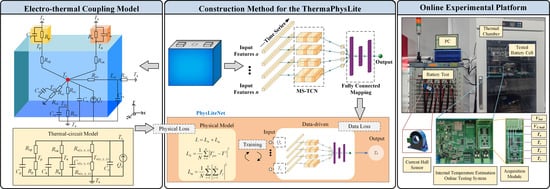
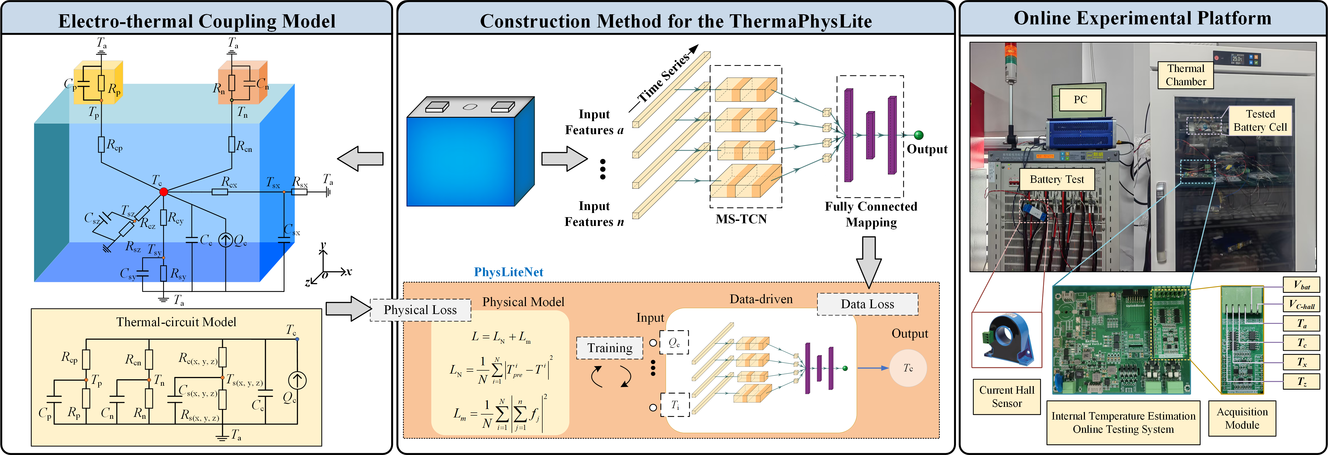
Graphical Abstract

1. Introduction

Lithium-ion batteries are widely used in electric vehicles, energy storage systems, and consumer electronics due to their superior performance. Temperature critically affects the performance and safety of lithium-ion batteries. At low temperatures, decreased electrochemical reaction rates and ion diffusion rates lead to capacity degradation [1]. Conversely, elevated temperatures exacerbate internal side reactions, accelerating battery aging and potentially leading to thermal runaway, resulting in fires and explosions [2]. Furthermore, temperature significantly influences the activity of battery materials, truth internal temperatures were obtained via side-drilling thermocouple embedding, impacting available power capacity, maximum charge–discharge speed, and rate of aging [3,4]. In addition, temperature is a key indicator of thermal runaway. When the rate of temperature increase exceeds a specific threshold, lithium-ion batteries can undergo thermal runaway, triggering a series of exothermic reactions [5]. The temperature difference between the surface and interior of a single cell can reach tens or even hundreds of degrees Celsius during high-rate charging or discharging [6]. Therefore, timely and accurate temperature monitoring is one of the most critical functions of a Battery Management System (BMS), while accurate estimation of internal cell temperature represents an important capability target for next-generation BMSs. Current BMSs typically employ thermocouples or resistance temperature detectors mounted on the battery surface to measure temperature. However, due to the temperature gradient between the battery surface and its interior, surface temperature measurements alone are insufficient. Consequently, internal battery temperature must be accurately estimated by leveraging other parameters and algorithms. It is worth noting that the present work is specifically motivated by stationary large-scale energy storage applications (e.g., grid-scale battery energy storage stations, BESS), where batteries operate within thermally controlled environments (typically 15–35 °C ambient) maintained by dedicated thermal management systems [7,8]. The methodology and validation scope of this work are accordingly bounded within this engineering context. Extension to scenarios involving significant ambient temperature drift (e.g., automotive applications) constitutes future work and is acknowledged in the Section 5.3 (Limitations).
Currently, there are three distinct approaches to battery temperature estimation: model-based, impedance-based, and data-driven methods. Model-based methods estimate internal battery temperature by establishing thermodynamic models (e.g., numerical models, electro–thermal models, and electrochemical-thermal models) and combining measurable parameters, such as voltage and current, with appropriate algorithms [9]. Although model-based methods generally offer high accuracy, they also entail significant modeling complexity and computational burden. Numerical battery models are typically described by nonlinear Partial Differential Equation (PDE) systems and boundary conditions. The accuracy and complexity of these models increase progressively from one-dimensional to three-dimensional representations. However, excessive complexity and computational cost can hinder practical applications. Therefore, when employing numerical battery models, rational simplification techniques are required to reduce the model order and approximate the PDEs, achieving a balance between accuracy and computational efficiency. Within this trade-off spectrum, lumped-parameter thermal models—such as RC thermal circuit models—occupy an attractive middle ground: they often achieve reasonable temperature estimation accuracy at significantly lower computational cost than full PDE-based numerical models, particularly when the engineering focus is on representative-point temperatures (e.g., core temperature and surface temperature) rather than fine-grained spatial distributions. This computational efficiency makes lumped-parameter approaches especially well-suited for edge-deployed BMS applications such as the one targeted in the present work. Electro–thermal models require both electrical circuit models and thermal circuit models to be established. They estimate the heat generation of the battery through parameters such as voltage and current, thereby solving for the internal battery temperature. While this approach can provide high accuracy, it also necessitates the identification of model parameters. Furthermore, many model parameters, for example, ohmic resistance, vary with temperature and State-of-Charge (SOC), making it challenging to simultaneously ensure both model generalization capability and computational efficiency. Reference [10] developed an electro–thermal model for a pouch cell with three heat sources. They calculated heat generation at the battery terminals and center position using a circuit model, and then derived the temperature distribution of the battery through a thermal circuit model and ambient temperature. Although this approach can obtain the temperature distribution of the entire battery, the resistances and capacitances in the model are subject to parameter identification by experiments, such as Hybrid Pulse Power Characterization (HPPC). These parameters change with temperature and SOC, which, in turn, affects the accuracy of temperature estimation. Reference [11] established a three-node electro–thermal model for a cylindrical battery, considering the impact of internal resistance and SOC variations on temperature estimation. This model can accurately estimate the radial temperature distribution; however, this also increases model complexity and computational burden. Furthermore, it requires Open-Circuit Voltage (OCV) calibration experiments and entropic coefficient calibration experiments, resulting in a substantial experimental workload. Reference [12] employed a physics-informed equivalent circuit model that considers the current dependence of the charge transfer resistance. The model parameters are continuously estimated using a dual extended Kalman filter to ensure the long-term validity of the equivalent circuit model. The thermal model is characterized using a physics-informed equivalent circuit model. Experiments show that this method maintains highly accurate temperature estimation over 800 full cycles, with a maximum RMSE of 1.2 °C.
Electrochemical Impedance Spectroscopy (EIS) contains information regarding battery temperature. Unlike voltage and current measurements, impedance spectra can fundamentally reflect the internal state of the battery. When battery temperature changes, processes such as diffusion and charge transfer also change within the battery, leading to alterations in the impedance spectra. Existing literature has explored battery temperature estimation based on the real part, imaginary part, modulus, and phase angle of impedance [13,14,15]. However, many studies focus on the relationship between impedance and the battery’s average bulk temperature, whereas a temperature gradient exists between the average bulk temperature and the internal temperature. Therefore, relying solely on impedance information can make it difficult to obtain an accurate estimation of the internal battery temperature. Reference [14] studied the relationship between impedance and SOC, SOH, and temperature, selecting impedance attributes that are weakly correlated with SOC but strongly correlated with temperature to estimate battery temperature. However, it can only estimate the bulk average temperature of the battery. Reference [15] theoretically derived the radial temperature distribution of a cylindrical battery, estimating internal battery temperature based on impedance and surface temperature. While this method is relatively simple and easy to implement, it does not consider the effect of ambient temperature on battery heat dissipation, and the generalization capability of the method remains to be verified. Reference [16] proposed a sensorless battery temperature estimation method that detects the zero-crossing frequency point of the battery phase. However, the accuracy of this method is generally limited, and it cannot characterize the non-uniformity of the battery temperature distribution. Furthermore, it requires frequency scanning, resulting in a slow response speed.
EIS is indeed a valuable characterization technique for the average bulk temperature of a battery. However, it typically requires integration with additional information or models to accurately estimate the battery’s internal temperature. Furthermore, for large-capacity cells, obtaining accurate impedance spectra can be challenging. Machine learning-based data-driven approaches are effective for battery temperature estimation, as they can accurately capture the nonlinear dynamics of battery systems. These methods have been widely applied in various battery state estimation applications. Reference [17] generated training data through an electro–thermal equivalent simulation model of the battery and employed a 2D Gated Long Short-Term Memory (GLSTM) model to learn the thermal characteristics of the battery. The proposed method generates the training set through simulation, which reduces the difficulty of data acquisition while providing high-quality data and achieving high temperature estimation accuracy. However, the electro–thermal model does not consider the influence of temperature and SOC on the parameters, and the ambient temperature of the training and test sets are identical. Therefore, the generalization ability of the model to actual operating conditions remains to be verified. Reference [18] extracted impedance features based on correlation coefficients and used a Support Vector Regression (SVR) model to learn the temperature characteristics of the battery, achieving high temperature estimation accuracy. However, it only estimated the average bulk temperature of the battery. Reference [19] proposed a method based on Long Short-Term Memory (LSTM) networks and Transfer Learning (TL) to estimate the internal temperature of lithium batteries. This method reduced the computational burden for estimating the internal temperature of other lithium batteries. The maximum RMSE obtained in the experiment was 0.3302 °C. Reference [20] proposed a Recurrent Neural Network (RNN) based on Gated Recurrent Units (GRU) to achieve high-precision battery surface temperature estimation. Reference [21] introduced a novel joint estimation method for battery internal temperature and SOC, which first estimates SOC through a 2D Convolutional Neural Network (2D-CNN), and then estimates internal temperature by combining the estimated SOC with collected voltage, current, and surface temperature information, verifying the effectiveness of classification-based deep learning methods in lithium battery internal temperature estimation applications.
Existing methods for estimating battery internal temperature struggle to simultaneously achieve high accuracy, low computational cost, and robust generalization performance. Model-based methods necessitate the identification of model parameters under various load profiles while maintaining a constant ambient temperature, leading to substantial computational and experimental burdens. EIS-based methods are less suitable for large-capacity lithium batteries due to the difficulty in accurately measuring impedance spectra. Data-driven methods require comprehensive, high-quality datasets.
To overcome the inherent limitations of purely data-driven deep learning methods in scientific computing and engineering applications, Karniadakis et al. proposed a novel framework based on deep learning for solving PDEs, termed PINN [22]. Researchers have since begun incorporating physical principles as constraints to enhance the physical interpretability of deep learning methods while simultaneously reducing the data requirements of deep learning models. Within the field of battery internal temperature estimation, several researchers have adopted Physics-Informed Machine Learning paradigms, exemplified by PINNs, and combined them with battery physics-based models to estimate battery internal temperature. Reference [23] estimated battery temperature based on a PINN, which incorporates the thermal equation into the loss function of a general neural network. This approach enables high-precision temperature prediction with limited amounts of data; however, it does not consider the difference between internal and external temperatures, and its network structure is complex, making the hyperparameters difficult to optimize. Reference [24] adopted the paradigm of PINNs, combining a battery thermal model, a temperature data preprocessing model, and a Multilayer Perceptron (MLP) network model to explicitly incorporate physical information into the neural network model. Empirical measurements demonstrated that the RMSE between the estimated temperature and the actual temperature obtained by this method is less than 0.8 °C. Reference [25] proposed a battery cell temperature estimation method based on a numerical model with an LSTM network. This technique extracts features from the numerical model, estimates the volume-averaged temperature through EIS, and uses an LSTM network to learn thermodynamic parameters and complex calculations. This approach leverages the strengths of each method to achieve accurate internal temperature estimation.
Despite the demonstrated potential of PINN methods for rapid and accurate battery internal temperature estimation, existing research predominantly focuses on algorithmic accuracy enhancement at the theoretical level. This often results in increasingly cumbersome and complex model structures, with a severe lack of consideration for deployment feasibility from an engineering perspective. Most existing PINN or deep learning models are developed and validated on high-performance GPU workstations, neglecting the critical constraint of extremely limited computing resources at the edge. This significant Engineering Gap between theoretical models and actual deployment environments severely hinders the industrial implementation of advanced algorithms.
This issue is particularly pronounced in large-scale energy storage system applications. These systems typically consist of thousands or even tens of thousands of battery cells, while commercial BMSs are constrained by cost and power consumption and therefore predominantly utilize low-end microcontrollers with limited computational power and memory. Direct deployment of complex deep learning models or high-order numerical models on such hardware is impractical. Although cloud-based solutions offer sufficient computing power, the transmission latency caused by long-distance communication links and the potential privacy risks associated with uploading data render them unsuitable for battery status monitoring tasks that demand high real-time performance and security. In contrast, edge computing, as a distributed computing paradigm that migrates data processing tasks to edge nodes near the data source, can effectively reduce latency, conserve bandwidth, improve real-time performance, and enhance data security, making it more suitable for large-scale energy storage applications.
To address the conflict between algorithmic precision and hardware constraints, this paper proposes ThermaPhysLite, a lightweight internal temperature estimation method that extends our preliminary work [26] into a more rigorous and complete framework. Distinguished from generalized models that pursue universal applicability, ThermaPhysLite adopts an engineering-oriented paradigm tailored to a specific deployment scenario—large-format prismatic LFP cells in thermally controlled stationary energy storage systems. Extension to other chemistries or form factors requires corresponding re-identification and re-training, as discussed in Section 5. By incorporating simplified physical constraints and focusing on stable operating environments (e.g., constant ambient temperature scenarios typical in data centers or grid storage), the proposed method achieves a significant reduction in computational load while maintaining high accuracy within its target domain. The methodology is structured as follows. First, physical constraints are formulated by constructing an electro–thermal coupled model. Redundant input variables are then trimmed through symmetry simplification and parameter identification results from the physical model. Second, a Temporal Convolutional Network (TCN) architecture is employed to learn the temporal transfer characteristics of temperature. Based on the parameter identification results of the physical model, an MS-TCN is designed, further optimizing the convolutional kernel size structure compared to traditional TCN. Third, the physical constraints of the electro–thermal coupled model are embedded into the training process of the MS-TCN through a PINN architecture. The physical information effectively guides the learning process of the neural network, thereby achieving enhanced performance with a reduced network size. The resulting model is specifically designed for edge computing in energy storage systems. Fourth, the ThermaPhysLite model is deployed on an ESP32-S3-based embedded platform using TensorFlow Lite. A prototype is designed, and online testing experiments are conducted to verify the operational efficiency and accuracy of the ThermaPhysLite model. This provides a novel method and engineering practice case for lithium battery state estimation in large-scale energy storage systems.

2. Principle of the Proposed Internal Temperature Estimation Method
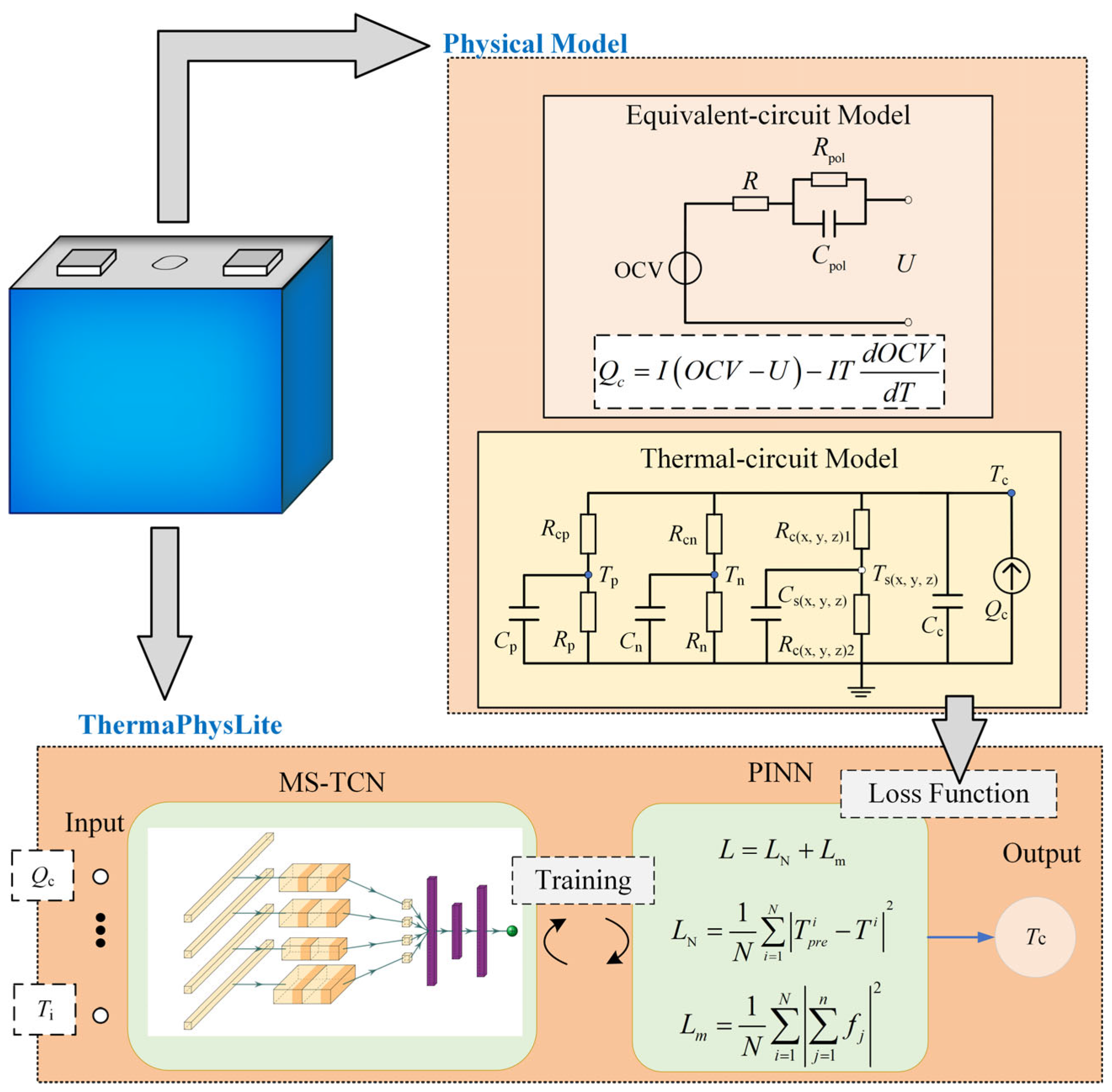
To address the limitations of existing temperature estimation methods, this paper proposes ThermaPhysLite, an edge computing model designed for large-scale energy storage systems. ThermaPhysLite estimates the internal temperature of lithium-ion batteries by integrating a PINN with an MS-TCN. The PINN incorporates physical constraints and data-driven features to guide the neural network towards adherence to physical laws, thereby enhancing learning accuracy and efficiency without increasing model complexity.
Common physics-informed elements include PDEs, Ordinary Differential Equations (ODEs), Stochastic Differential Equations (SDEs), system constraints, and intuitive physical principles. These can be embedded into various components of a neural network, including data processing, network architecture, loss functions, optimization methods, and inference algorithms. In this work, physical equations are extracted from the battery’s physical model to construct a physics-informed loss function. Additionally, based on parameter identification results from the physical model, the number of input variables for the neural network is reduced, thereby simplifying the model.
This approach effectively leverages prior knowledge from physical models while utilizing the MS-TCN to learn unknown parameters and complex computations. Consequently, it enables accurate internal temperature estimation at the edge with limited data and a lightweight model structure.
Figure 1 illustrates the construction of the proposed ThermaPhysLite framework, which consists of two primary components: 1. Development and simplification of the electro–thermal coupling model. 2. Establishment and training of the ThermaPhysLite model.
Figure 1. Schematic diagram of the construction method for the ThermaPhysLite temperature estimation model. The battery icon (top left) denotes the prismatic Li-ion cell under study, from which two gray block arrows indicate the flow of information to the two main branches of the framework: the Physical Model and the data-driven ThermaPhysLite model. In the Physical Model panel, the upper part shows two alternative heat-generation formulations—the equivalent-circuit model and the Bernardi equation (boxed)—of which the Bernardi equation is adopted in this work; the lower part shows the simplified thermal-circuit model of the prismatic battery (corresponding to Figure 2d). In the ThermaPhysLite panel, the dashed box on the left lists the model inputs (Qc, Ta, Tsx, Tsz); the central block illustrates the proposed MS-TCN architecture; the curved “Training” arrow denotes the iterative optimization process; the right block shows the PINN-based loss function combining the network loss LN and the physics-based loss Lm; and the blue arrow on the right indicates the model output, the internal temperature Tc. The gray block arrow from the Physical Model panel to the Loss Function indicates that physical constraints derived from the electro-thermal coupling model are embedded into the network training as a regularization term. Definitions of all symbols are given in Table 1.
Batteries 12 00189 g001
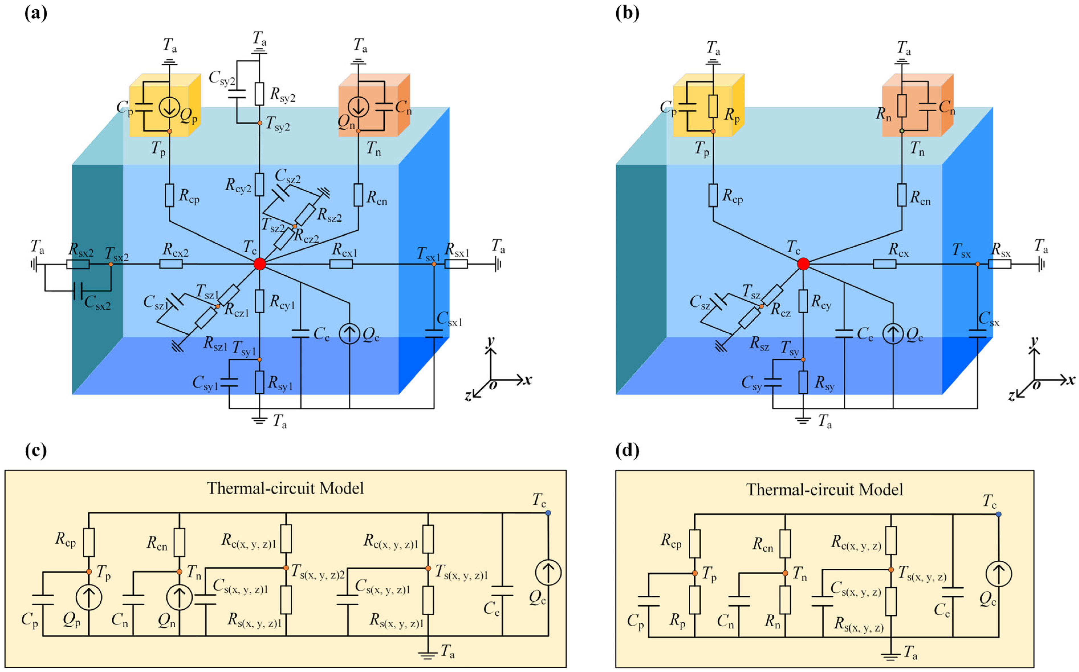
Figure 2. Electro-thermal coupling model of the prismatic battery: (a) 3D structure of the high-order model; (b) 3D structure of the simplified model; (c) high-order thermal circuit diagram; (d) simplified thermal circuit diagram. In (a,b), the yellow block denotes the positive tab of the battery, the orange block denotes the negative tab, and the blue body represents the battery cell. The red dot marks the internal temperature node Tc, and the orange dots mark the temperature nodes on the corresponding outer surfaces of the cell. Definitions of all symbols are given in Table 1.
Batteries 12 00189 g002
Table 1. Parameter definitions for the electro–thermal coupling model (Equations (3)–(9)).
SymbolDescription
QcInternal heat generation rate of the cell (Bernardi equation)
TcCore (internal) temperature
TaAmbient temperature
Tp, TnPositive/negative tab surface temperatures
Tsx, Tsy, TszSurface temperatures along x, y, z directions
CcThermal capacitance of cell core
Cp, CnThermal capacitances of positive/negative tabs
Csx, Csy, CszThermal capacitances of surface nodes
Rp, RnTab-to-ambient thermal resistances
Rcp, RcnCore-to-tab thermal resistances
Rcx1, Rcy1, Rcz1Core-to-surface thermal resistances (x, y, z)
Rcx2, Rcy2, Rcz2Surface-to-ambient thermal resistances (x, y, z)

2.1. Development and Simplification of the Electro–Thermal Coupling Model

Training neural networks solely using experimental data requires a large amount of high-quality data. By incorporating prior knowledge or physical models, the model can achieve better performance even with limited data and a simplified structure. Based on the thermal circuit model of a prismatic battery, this work applies appropriate approximations to reduce the number of parameters to be identified, thereby lowering model complexity. The extracted thermal model is then formulated as a loss function and integrated into an MS-TCN to enhance learning efficiency. The foundational modeling approach was initially explored in [26]; the present work substantially extends it by incorporating a higher-order thermal circuit, systematic parameter identification experiments, and a rigorous analysis of the physical rationale for constant-parameter assumptions.
Figure 2a illustrates the high-order equivalent thermal circuit model of a prismatic battery. This model is developed based on heat transfer principles and accounts for the anisotropic geometric structure of the battery through discrete modeling along the x-, y-, and z-axes. By leveraging structural symmetry, the temperature distribution at symmetric positions in each direction is assumed to be identical. The model differentiates between the metallic tab materials and the electrochemically active materials in the battery body. Given the substantial Joule heating generated by contact resistance, the positive and negative tabs are treated as independent heat source nodes, with their respective heat transfer processes to the ambient environment and battery body explicitly described.
Although the aforementioned high-order model captures the non-uniform internal temperature distribution and tab thermal effects through refined discretization, deploying such a complex model on resource-constrained edge devices (e.g., BMS slave modules) in large-scale energy storage systems presents dual challenges in computational capacity and cost. Adhering to the engineering principle that complexity does not necessarily ensure effectiveness, this paper performs model simplification tailored to edge computing scenarios.
Surface Measurement Point Simplification: Although temperature gradients exist on the actual battery surface, limited by sensor deployment costs and data acquisition channel constraints in practical engineering, the external measurement points are symmetrically reduced to three key points: one temperature sensor is placed at the geometric center of the surface along the x-, y-, and z-directions, respectively. Quantitatively, this reduces the surface measurement nodes from six (Tsx1, Tsx2, Tsy1, Tsy2, Tsz1, and Tsz2 in the high-order model) to three (Tsx, Tsy, and Tsz in the simplified model), with the associated thermal resistance/capacitance pairs reduced from twelve to six.
Tab Heat Transfer Simplification: Given that the battery tabs are composed of high-thermal-conductivity metals and connected via copper busbars, heat is easily dissipated to the environment; thus, their heat conduction influence on the battery interior is approximated as negligible. Specifically, the tab heat source terms (Qp, Qn) in the high-order model are removed, while the tab thermal capacitances (Cp, Cn) and the thermal resistance pathways (Rp, Rn, Rcp, Rcn) connecting the tabs to the core and ambient are retained as passive conduction nodes.
Heat Source Simplification: To adapt to the computational resource constraints of large-scale energy storage scenarios, the complex internal electrochemical heat generation of the battery is approximated as a single central concentrated heat source. Concretely, this consolidates the distributed multi-source representation into a single central heat source Qc, computed via the Bernardi equation.
It is worth noting that the single-source simplification adopted here is consistent with both physical observations and engineering practice for large-format prismatic cells. Recent investigations on large-capacity prismatic energy storage batteries have shown that the position of maximum heat generation progressively migrates from the tab-near region toward the central jellyroll region during sustained discharge [27], indicating that the overall thermal response is dominated by the central region rather than by localized tab heating. Furthermore, the metallic tabs are connected to high-thermal-conductivity busbars that efficiently dissipate tab-region heat directly to the ambient air, minimizing their contribution to the internal cell temperature field [28]. The empirical parameter identification results presented in Section 3.2 provide additional support: the tab-derived temperature estimates (Tc1, Tc2) yield identification RMSE values that are an order of magnitude worse than surface-derived estimates, confirming that the tab pathway is not well-suited as a primary internal temperature inference route. Any residual error introduced by this simplification falls within the short-term variation regime that the MS-TCN component is designed to compensate for (Section 2.2).
Through these simplifications, the reduced-order prismatic battery thermal circuit model depicted in Figure 2b is established. Meanwhile, the high-order and simplified thermal circuit models are illustrated in Figure 2c and Figure 2d, respectively. This model requires only five external temperature inputs from the x-, y-, and z-direction surfaces and the positive and negative tabs, preserving essential thermal dynamics while significantly decreasing computational complexity.
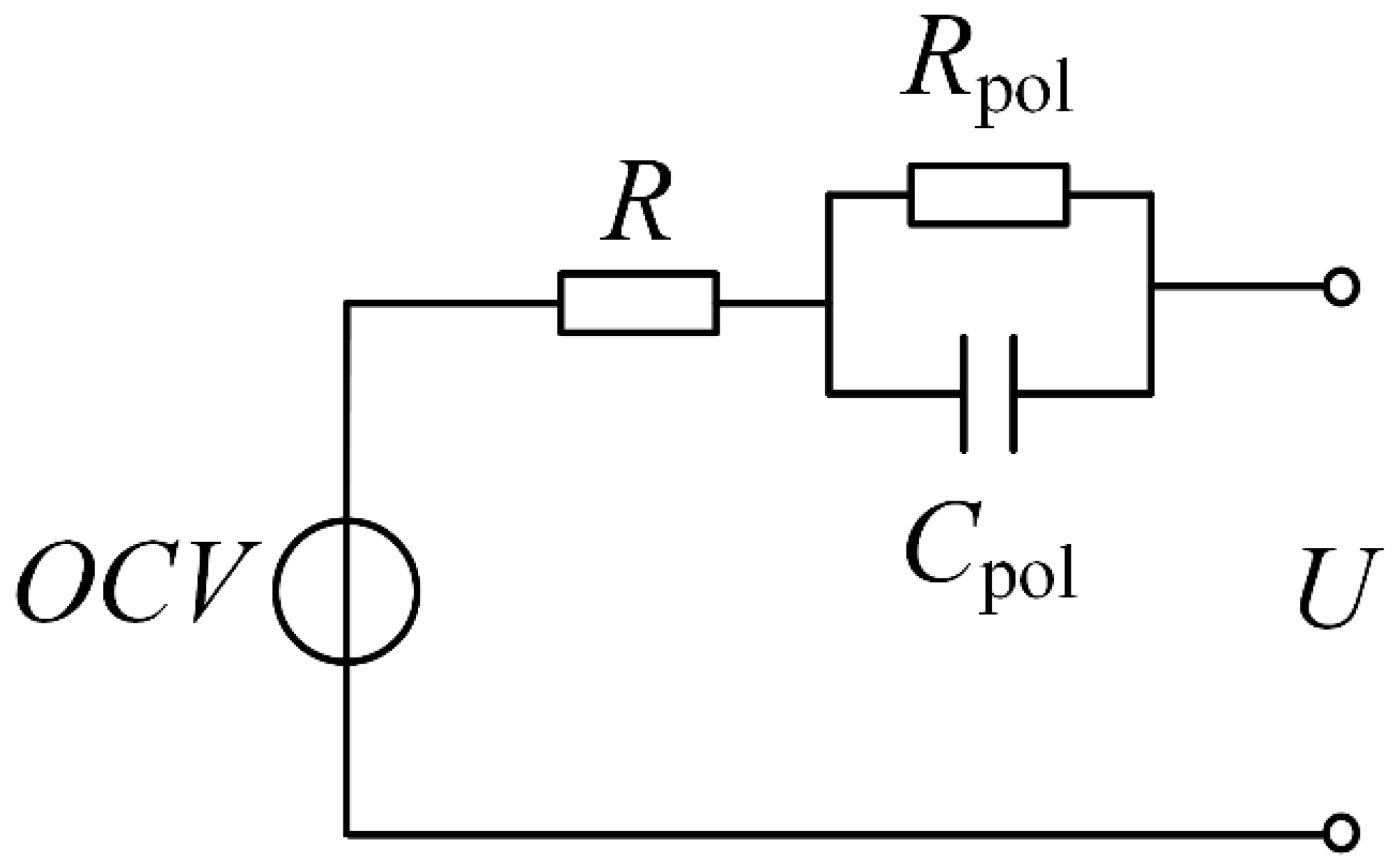
The heat source Qc in the thermal circuit model shown in Figure 2d cannot be directly determined from the thermal circuit itself; it must be obtained from the equivalent circuit model of the lithium-ion battery. The solved heat source Qc is then incorporated into the thermal circuit model, enabling the estimation of temperatures at various points. Regarding the calculation of heat source Qc, since the heat sources at the tabs have been simplified, the battery’s heat generation model can be simplified from a three-heat-source model to a single internal heat source model. This single heat source can be approximated using a first-order equivalent circuit model of the lithium-ion battery, as illustrated in Figure 3.
For the obtained first-order equivalent circuit, online parameter identification methods can be employed to identify the resistance and capacitance parameters of the equivalent circuit in real time. Subsequently, Joule’s law is applied to calculate the battery’s heat generation.
Q c = I 1 2 R + I 2 2 R p o l
where Qc represents the heat generation rate of the battery, I1 is the current flowing through resistor R, and I2 is the current flowing through resistor Rpol. It should be noted that Equation (1) is presented here for completeness in describing the ECM-based heat estimation methodology; however, this approach is not adopted in our actual implementation due to the limitations discussed below. The proposed ThermaPhysLite uses the Bernardi equation (Equation (2)) for heat generation calculation throughout both training and inference.
The method of obtaining the battery’s internal heat generation through online identification is highly real-time, accurate, and generalizable. However, it suffers from high computational complexity. In practical engineering applications, complex environmental noise can degrade its accuracy.
Therefore, this study employs the Bernardi heat generation equation to determine the battery’s internal temperature. The Bernardi equation is expressed as follows:
Q c = I O C V U I T d O C V d T
where I is the battery charge–discharge current, T is the battery temperature, U is the battery terminal voltage, and OCV is the open-circuit voltage. Qc is as defined in Equation (1).
Using the Bernardi equation to determine the battery’s heat generation rate requires establishing the functional relationship between OCV and SOC. It also necessitates obtaining the derivative of OCV with respect to battery temperature T to determine the polarization and reaction heat. This involves recording the OCV corresponding to different SOC values at various temperatures. Consequently, the internal heat generation Qc can be calculated from the battery charge–discharge current I, terminal voltage U, and SOC.
It is worth emphasizing that the aforementioned simplification scheme is not a compromise in physical model accuracy, but an optimized design for large-scale energy storage system application scenarios. In actual energy storage systems, batteries are typically standardized cells produced in large-scale batches, possessing high consistency in manufacturing processes and structural parameters, which to some extent provides an engineering basis for lumped parameter modeling. Furthermore, in large-scale energy storage systems, model complexity does not necessarily equate to improved prediction performance. Compared to high-dimensional distributed parameter models, a thermal circuit model with a concise structure and clear physical meaning is more conducive to online deployment, parameter identification, and fusion with data-driven models. Therefore, by appropriately simplifying the thermal circuit structure, this paper enhances the model’s practicality and scalability in complex engineering scenarios while ensuring physical rationality.
Based on the preceding analysis, a prismatic lithium-ion battery electro–thermal coupled model suitable for online internal temperature estimation is formulated. The mathematical expressions are given as follows:
Q c = I O C V U I T d O C V d T
C p d ( T p T a ) d t = T a T p R p + T c T p R cp
C n d ( T n T a ) d t = T a T n R n + T c T n R cn
C cx d ( T sx T a ) d t = T c T sx R cx1 + T a T sx R cx2
C cy d ( T sy T a ) d t = T c T sy R cy1 + T a T sy R cy2
C cz d ( T sz T a ) d t = T c T sz R cz1 + T a T sz R cz2
C c d ( T c T a ) d t = T p T c R cp + T n T c R cn + T sx T c R cx1 + T sy T c R cy1 + T sz T c R cz1 + Q c
Before discussing the parameter assumptions in detail, it is important to distinguish between two fundamentally different categories of parameters in the proposed electro–thermal coupled model:
(i)
Heat generation parameters: These include the OCV, the entropic coefficient dOCV/dT. These parameters are inherently SOC-dependent and are explicitly modeled as functions of SOC in our framework (see Section 3.2).
(ii)
Heat dissipation parameters: These include the thermal resistances and thermal capacitances in the thermal circuit model (Equations (4)–(9)). These parameters describe heat transfer pathways and intrinsic material thermal properties, which are governed by the battery’s geometric configuration and material thermophysical characteristics—not by the electrochemical state of charge.
The constant-parameter assumption discussed in the following paragraphs applies specifically to category (ii). The SOC dependence of category (i) parameters is explicitly handled through the experimental fitting in Section 3.2.
Unlike purely mathematical fitting models, thermal resistance R and thermal capacitance C are not abstract fitting parameters but thermodynamic quantities with clear physical meanings. Thermal resistance R characterizes the resistance encountered during heat transfer from the battery core to the surface, reflecting the magnitude of the spatial temperature gradient; thermal capacitance C characterizes the ability of battery materials to absorb heat, embodying the time lag and thermal inertia of the battery’s temperature response.
With respect to parameter stability, adopting constant thermal parameters is a widely accepted simplification in electro–thermal modeling, as validated by previous studies where similar models utilizing constant thermal resistance and capacitance achieved high estimation accuracy [29,30]. Quantitative evidence further supports this assumption. Literature [31] indicates that within the typical operating range of 15 °C to 35 °C, the specific heat exhibits marginal fluctuation of less than 5% (ranging from approximately 1143 to 1190 J·kg−1 °C−1). Moreover, research has confirmed that the heat dissipation parameters (thermal resistances and capacitances) of lithium-ion batteries are effectively independent of the State of Charge (SOC) [32], as these parameters are governed by geometric and material thermophysical properties rather than by the electrochemical state. As thermal resistances and capacitances are fundamentally dictated by the battery’s geometric configuration and material thermophysical properties, these parameters can be regarded as quasi-invariant with respect to operating condition fluctuations during typical charge and discharge cycles. This provides a solid physical rationale for adopting constant mean parameters to describe the thermal dynamics in our model.
After obtaining all parameters in Equations (3)–(9), the battery internal temperature can theoretically be calculated. However, as previously mentioned, thermal resistance and capacitance are, strictly speaking, non-linear parameters that vary with temperature and SOC. Although this variation is relatively small within the ambient temperature range, this paper does not evade the objective existence of parameter variations but addresses this challenge through the unique mechanism of the PINN framework.
In this method, the simplified physical equations play a role primarily during the training phase, specifically by internalizing the thermodynamic conservation laws into the neural network weights via the physics-informed loss term. The physical model here acts as a regularization constraint, guiding the network to search for optimal solutions within the solution space that conform to physical laws. In the inference phase, the fixed physical parameters no longer explicitly participate in the calculations; at this point, the trained network weights already embody the physical laws. More importantly, the pure data-driven part of the neural network possesses powerful non-linear mapping capabilities, enabling it to learn and partially compensate for the residuals caused by static parameter assumptions and unmodeled dynamic characteristics. Therefore, in essence, the physical model provides a theoretical boundary based on average parameters, while the data-driven part performs refined non-linear corrections on this basis, ensuring that the final prediction results maintain physical consistency while possessing robustness against minor parameter variations.

2.2. Construction and Training of the ThermaPhysLite Model

TCNs represent a time series processing approach founded on Convolutional Neural Networks (CNNs). TCNs employ causal convolutions to ensure causality between time steps, while incorporating dilated convolutions to capture dependencies in long time series. The primary mathematical expression is given as follows:
y t = k = 0 K 1 x t d × k w k ,     t 0
where y(t) is the output sequence, K is the kernel size, w is the kernel, x(t) is the given input sequence, and d is the dilation factor. The purpose of the dilation factor is to expand the receptive field of the convolutional operation on the input sequence. To ensure the causality of the model, causal convolutions are employed, which are achieved through appropriate truncation of the convolutional kernel. Finally, the final output y of the TCN is obtained by further processing the output of the last layer, typically using a fully connected layer to derive the desired result.
Based on the physical model analysis, the feature sequence input to the TCN includes the battery heat generation rate Qc(t) and multi-point surface temperatures Ti (t) (where I = n, p, x, y, z; the number of surface temperature measurement points can be reduced based on experimental results to further simplify the model). Additionally, as indicated by Equations (4)–(9), ambient temperature significantly influences battery heat dissipation and temperature. Therefore, the ambient temperature Ta(t) is also included as an input feature variable. The output is the lithium-ion battery’s internal temperature Tc, which is a single feature value.
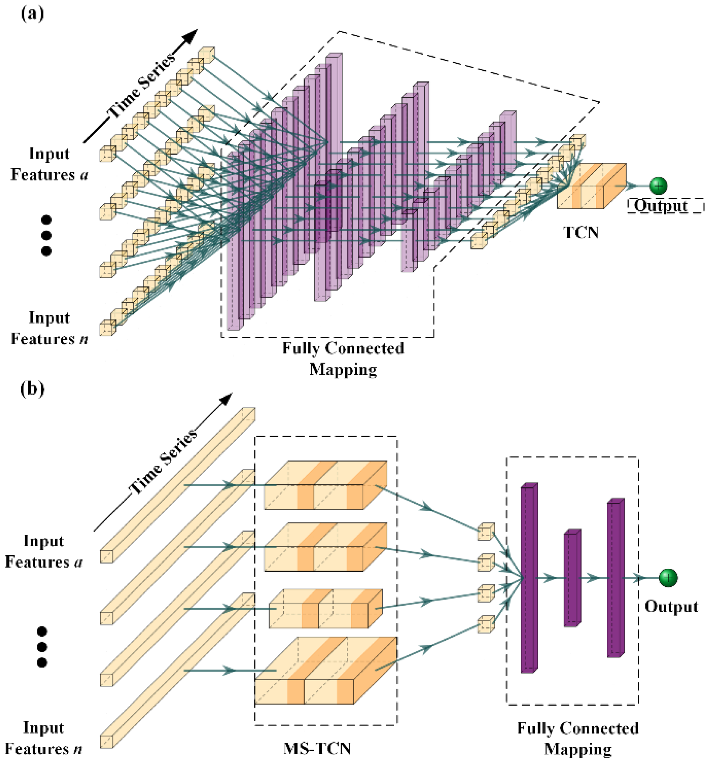
Given that the required network is designed for multi-feature sequence input and single feature value output, this study designed two network architectures tailored to the specific problem. Network architecture I, illustrated in Figure 4a, initially employs a fully connected layer to fuse all features acquired at the same time instant. Subsequently, temporal convolution operations are performed on the fused feature sequence. Finally, the temporal features resulting from multiple sets of convolutional kernel operations are subjected to fully connected mapping to obtain the internal temperature estimation result. This network architecture fuses features in the feature dimension before performing convolutional operations in the time series dimension. While this approach reduces the complexity of the convolutional operations, it overlooks the different time constants associated with the influence of different input features on the internal battery temperature. This simplification increases the complexity of the fully connected layer used for feature dimension fusion, as the fully connected layers required for feature fusion vary across different time instants in the time series. This ultimately increases the parameter complexity of the overall network model.
In contrast, Network Architecture II (MS-TCN), first introduced in [26] and further refined in this work, is explicitly designed to align with the physical thermal dynamics of the battery. Thermal conduction is inherently characterized by distinct hysteresis and inertia that depend on the heat source location and conduction pathways. Specifically, ambient temperature and surface temperatures influence internal temperature through relatively slow heat diffusion processes within the battery materials, thereby acting as slow-varying inputs with large time constants. Conversely, the internal heat generation rate serves as a direct source term, inducing rapid responses in the internal temperature field.
To capture these multi-scale thermal dynamics, Architecture II employs a multi-scale temporal convolution strategy. For the slow-varying input sequences (e.g., ambient and surface temperatures), larger convolutional kernel sizes and dilation factors are employed to expand the temporal receptive field, enabling the network to capture long-term dependencies and thermal lag effects. For the fast-varying input sequence (heat generation rate), smaller kernel sizes are adopted to preserve instantaneous variations and prevent excessive temporal smoothing of rapid thermal transients. The extracted temporal features from these multiple scales are subsequently fused and mapped to the final temperature prediction, as illustrated in Figure 4b.
Rather than calculating kernel sizes rigidly from fixed physical parameters, this study uses the estimated thermal time constants as heuristic guidance for determining the hyperparameter search range. This physics-inspired approach ensures that the network structure adheres to the laws of physics while avoiding the rigidity of purely model-based methods.
It is worth emphasizing that the proposed ThermaPhysLite hybrid architecture is designed to mitigate the impact of short-term parameter variations and unmodeled dynamics within its target operational envelope. In purely physics-based modeling approaches, fixed thermal parameters (i.e., thermal resistances and capacitances) cannot capture short-term variations associated with operating condition fluctuations.
In contrast, the MS-TCN within ThermaPhysLite operates as a powerful nonlinear compensator: while physical constraints based on average parameters provide approximate theoretical boundaries, the data-driven TCN layer compensates for residuals introduced by short-term parameter variations and unmodeled fast dynamics by learning residual patterns within the training distribution. This integrated approach is well-suited for stationary BESS applications operating within thermally controlled environments and within the typical health window. Long-term parameter drift caused by battery aging beyond the training distribution lies outside the inherent compensation scope of the MS-TCN; addressing such full-lifecycle drift requires the periodic model update strategy outlined in Section 5 (Future Work).
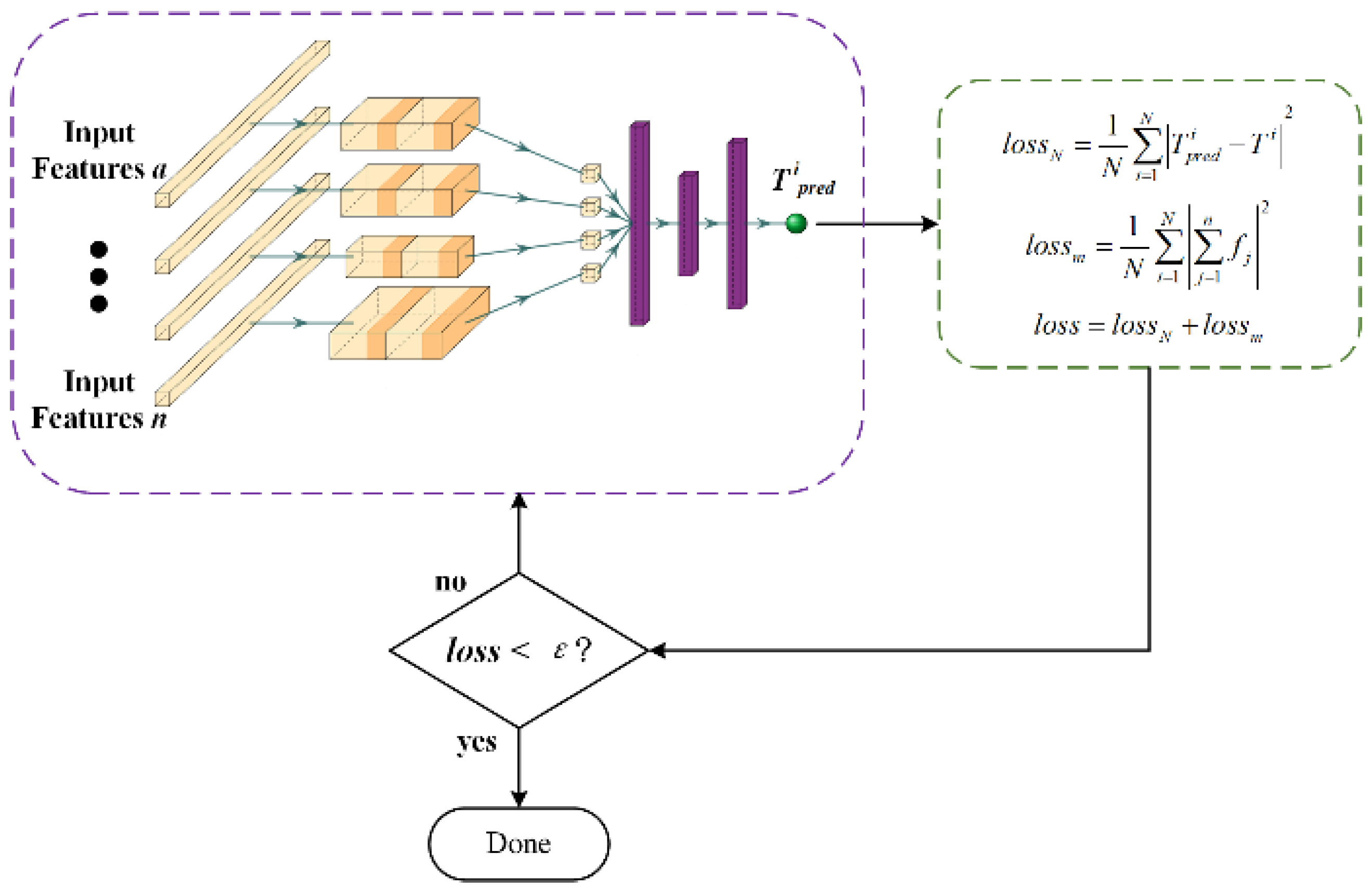
PINNs represent an emerging modeling paradigm that integrates deep learning with physical laws. Unlike traditional numerical methods (such as Finite Difference Method (FDM) or Finite Volume Method (FVM)) that rely on grid discretization to solve PDEs, PINNs utilize the universal approximation capability of neural networks to directly fit the non-linear mapping relationship among battery internal temperature, external measurement point temperatures, and heat generation rate, embedding physical governing equations as prior constraints into the training process. This study adopts the aforementioned MS-TCN as the backbone network; its core idea is to enforce satisfaction of physical laws while fitting experimental data by constructing a composite loss function.
To explicitly quantify this training objective, a composite loss function incorporating both data fidelity and physical consistency is constructed, as shown in Equations (11)–(13):
l o s s = λ N l o s s N + λ m l o s s m
l o s s N = 1 N i = 1 N T p r e d i T i 2
l o s s m = 1 N i = 1 N j = 1 n f j 2
where N is the number of samples in a mini-batch. Here, λN and λm are non-negative weighting coefficients that balance the contributions of the data fidelity term and the physics-informed regularization term, respectively. As widely documented in the PINN literature [33], the gradient magnitudes of physics-residual terms can differ substantially from those of data terms, leading to so-called gradient pathology issues during optimization. To mitigate this, λN is assigned a dominant weight, while λm is set to a smaller scale, ensuring that the physics-informed term provides effective regularization without overwhelming the data fidelity signal. The specific values of λN and λm were determined empirically by monitoring convergence behavior on the validation set, following common practice in PINN training [23]. Empirically, weight configurations within a moderate range yielded comparable convergence and final accuracy, suggesting the model is robust to precise weight selection within this regime.
The first term lossN is the data-driven loss, calculated as the Mean Squared Error (MSE) between the network-predicted internal temperature T p r e d i and the experimentally measured ground truth T i , ensuring the model captures the statistical patterns of the observed data.
The second term lossm is the physics-informed regularization term. Here, f j corresponds to the residuals of the physical governing equations formulated in Section 2.1 (Equations (4)–(9)). Specifically, the transient and thermal exchange terms from both sides of the differential equations are combined algebraically to compute the residual magnitudes. By minimizing the magnitude of these residuals, the optimization algorithm penalizes predictions that violate the conservation of energy. Ultimately, the total loss function loss drives ThermaPhysLite to find an optimal equilibrium solution between sparse experimental data points and continuous physical dynamic constraints, ensuring both accuracy and physical interpretability.
In summary, ThermaPhysLite achieves a deep synergy between physical mechanisms and data-driven learning, as illustrated in Figure 5. In the structural design phase, an MS-TCN architecture is customized based on the thermal dynamic differences in input features; in the model training phase, the simplified physical model is internalized as a loss function constraint via the PINN paradigm. This dual-integration strategy not only endows the model with the ability to leverage prior physical knowledge but also retains the neural network’s adaptability in handling parameter uncertainties and unmodeled dynamics, thereby guaranteeing the model’s generalization performance under variable operating conditions.

3. Experimental Design and Offline Model Validation

3.1. Experimental Environment and Preparations

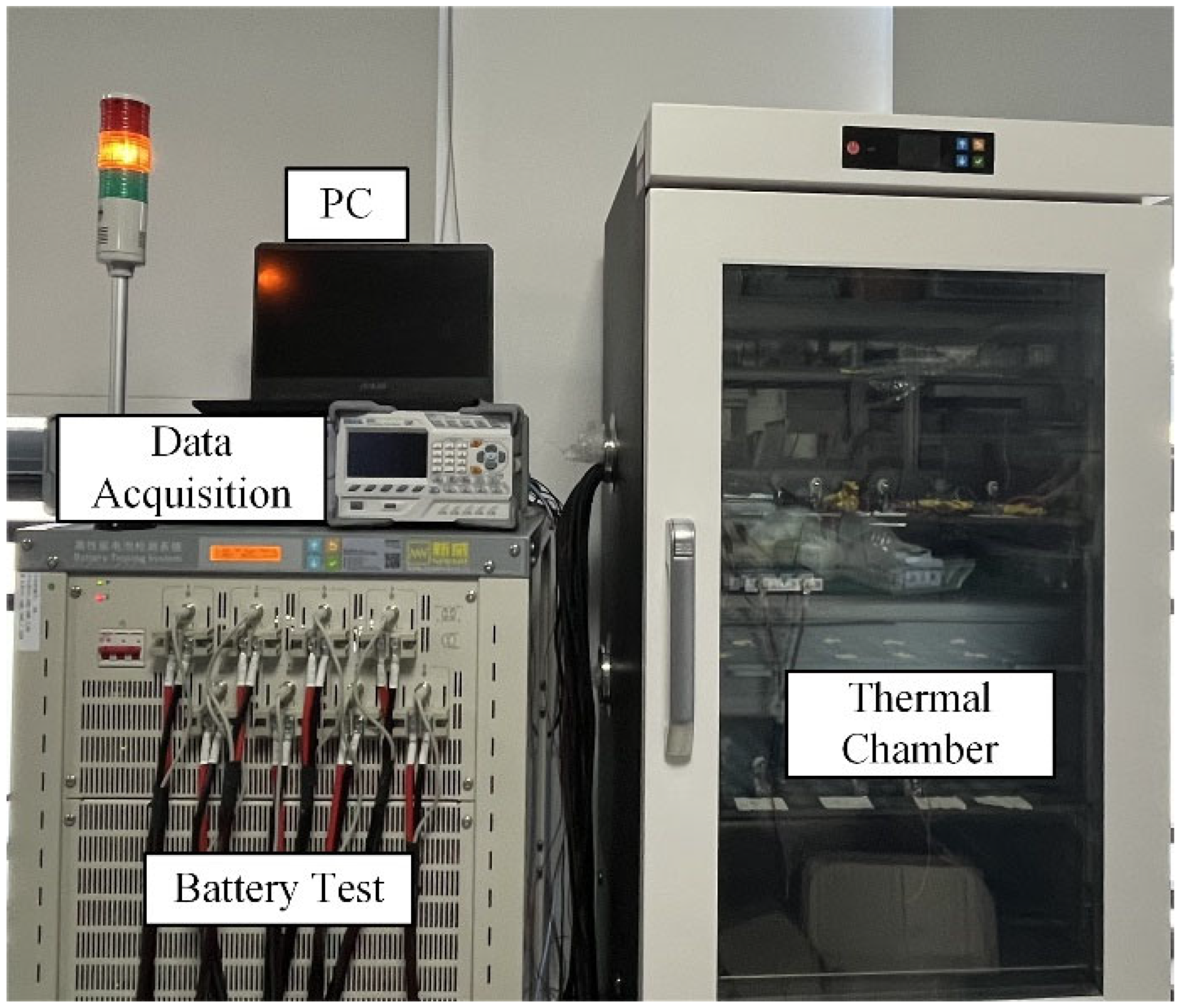
The experimental platform established in this study is shown in Figure 6. The research object is an EVE Energy LF105 prismatic hard-shell (EVE Energy Co., Ltd., Huizhou, China) Lithium Iron Phosphate (LFP) battery with a rated capacity of 105 Ah, a nominal voltage of 3.2 V, a charging cut-off voltage of 3.65 V, and a discharging cut-off voltage of 2.5 V. The battery charge–discharge cycler is a CT-4008-5V60A-NTA manufactured by NEWARE, (Shenzhen, China) which can use a multi-channel parallel method to make its charge–discharge current reach a maximum of 240 A, and the charge–discharge voltage range is 0 to 5 V. It can perform charge–discharge experiments on the battery under different working conditions and adjust the state of charge of the battery. The data acquisition system is an M300 data acquisition system produced by RIGOL, which is used to collect thermocouple temperature data from both the battery interior and multiple surface points. The temperature chamber (MHWX-2000) is manufactured by NEWARE, and its temperature adjustment range is 0 °C to 60 °C, which is used to control the ambient temperature in the experiment.
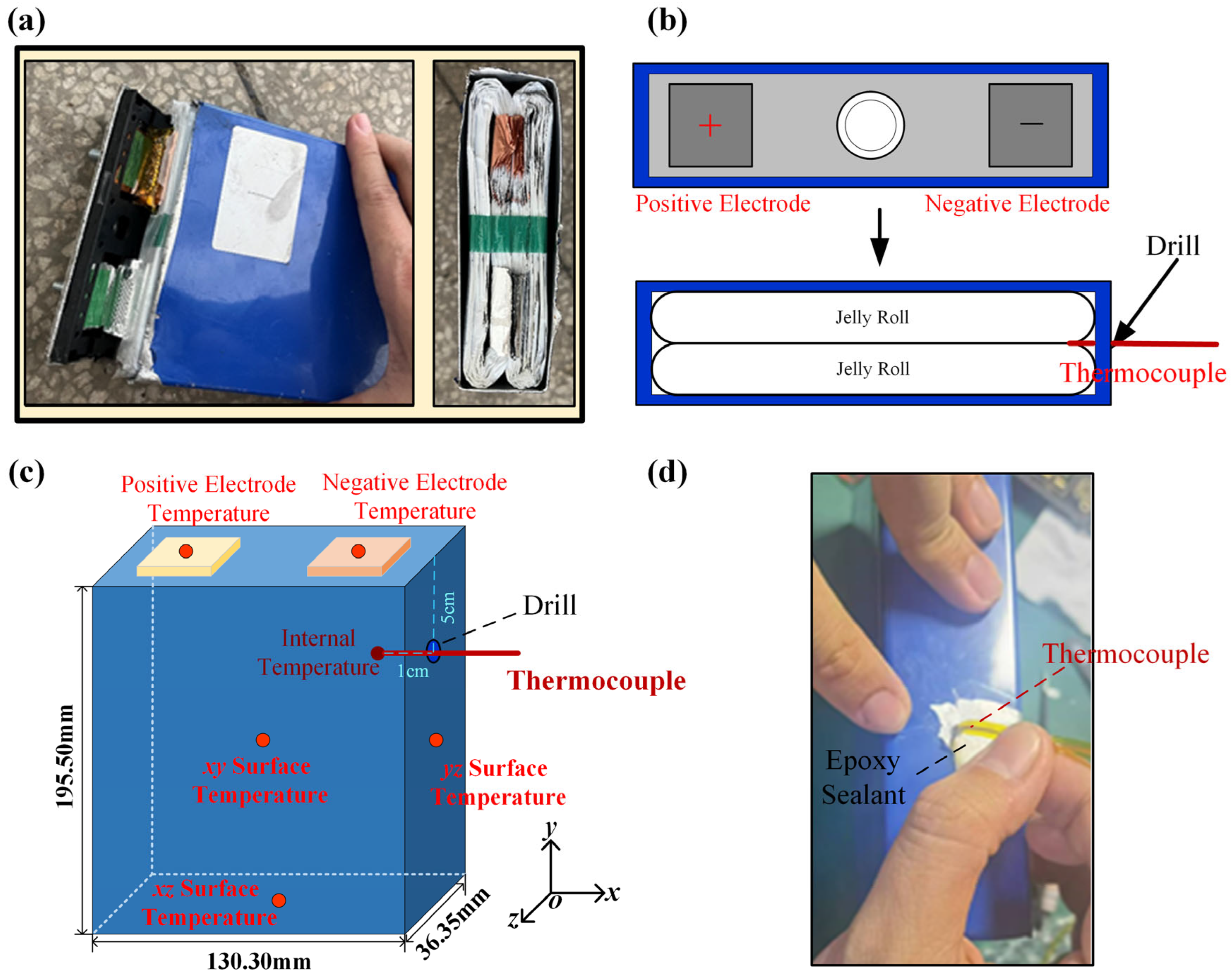
To measure the internal temperature of the battery, it is necessary to embed thermocouples without affecting the internal structure of the battery as much as possible. This requires disassembling the battery and fully understanding its internal structure before formulating an internal sensor embedding plan. The overall process is shown in Figure 7. First, a battery of the same batch and model is selected, and one of the batteries is discharged to SOC = 0. The battery is then disassembled. After disassembly, it is found that the battery has a double-layer winding core structure, as shown in Figure 7a. The winding core above the battery is densely wound, and there is no space for embedding a thermocouple. However, there is a gap in the crevice between the two winding cores on the side of the battery to embed the thermocouple. Therefore, this study uses a side-drilling method to implant the thermocouple from the side of the battery into the inside of the battery, so that it is close to the surface of the inner winding core of the battery. This step is carried out in a dry and clean environment as much as possible to prevent impurities or moisture from entering the battery. In terms of sensor selection, sensors with small diameters should be selected as much as possible to reduce the difficulty of sensor installation and its impact on the battery. The corresponding experimental steps are as follows:
First, discharge the target battery to SOC = 0. Then, use a small drilling machine to drill a hole on the side of the battery’s negative electrode, on the central axis near the top end cover. Bury an insulated K-type thermocouple into the center of the battery, as shown in Figure 7b,c. Finally, use epoxy sealant to seal the battery, as shown in Figure 7d. Capacity tests performed before and after the thermocouple embedding procedure showed that the battery capacity decreased from approximately 110 Ah (pre-embedding) to approximately 109 Ah (post-embedding), corresponding to a relative reduction in less than 1%. This change is within the typical cell-to-cell capacity variation observed across nominally identical commercial cells, and therefore the impact of burying the thermocouple on the battery is considered negligible for the purpose of internal temperature estimation validation.
It is worth noting that, due to the limitations of the existing ex situ preparation conditions in the laboratory, this study could not pre-embed sensors directly at the geometric center of the battery or the theoretical thermal hotspot during the winding or stacking production process, as battery manufacturers do. Existing studies indicate that these locations are typically the most significant areas for battery heat accumulation [34].
Nevertheless, the sensor implanted via side-drilling in this paper penetrates the gap between the two winding cores and is in close contact with the core surface, enabling sensitive and effective capture of the battery’s internal thermal dynamic response characteristics. For validation of the ThermaPhysLite online estimation approach, the experimental configuration provides sufficiently accurate ground-truth internal temperature data serving as validation references. Although this invasive post-processing method has physical limitations, it fully demonstrates the potential of the proposed estimation algorithm in capturing internal thermal dynamics. Furthermore, our team plans to explore sensor embedding techniques deeply integrated with battery manufacturing processes or use multi-physics simulations to assist in determining more precise hotspot locations in future research, thereby further enhancing the comprehensiveness of verification experiments.

3.2. Lithium Battery Heat Generation Estimation and Thermal Circuit Parameter Identification

The calculation of the heat source Qc in the electro–thermal coupling model constructed in Section 2.1 requires the relationship between battery SOC and OCV. The measurement of the OCV was mainly carried out with reference to the battery manual, and the experimental steps are as follows:
(1)
Set the temperature inside the constant temperature chamber to 25 °C;
(2)
Discharge the battery to SOC = 0, let it stand for 2 h, and record the OCV;
(3)
Perform constant current charging at 0.5C for 12 min, let it stand for 30 min, and record the OCV;
(4)
Repeat step (3) until the SOC increases to 100%;
(5)
Set the temperature inside the constant temperature chamber to 30 °C and then 35 °C, and repeat steps (2) through (4);
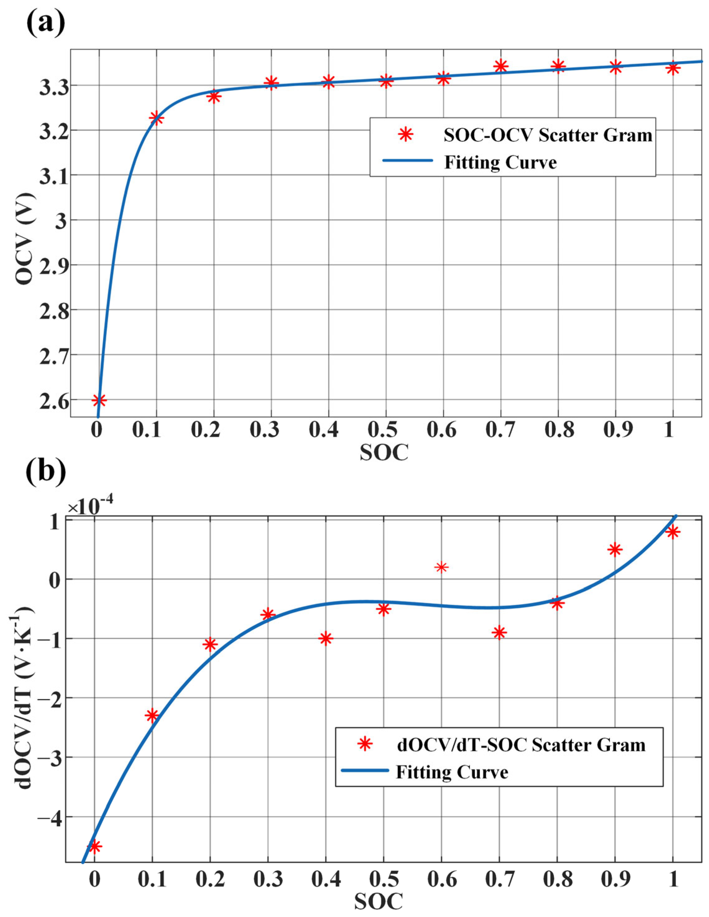
A second-order exponential equation was used to fit the functional relationship between SOC and OCV at 25 °C, as shown in Figure 8a. The expression is:
O C V = 3.2773 e 0.0217 × SOC 0.6808 e 24.3960 × SOC
Goodness-of-fit: R2 = 0.9987.
References [35,36] indicate that within the normal operating temperature range, the entropy coefficient is primarily dominated by SOC variations and exhibits low sensitivity to temperature changes. Similarly, the drift of the OCV curve with temperature is relatively weak in the ambient temperature range. Therefore, calculating the heat generation source Qc under all operating conditions based on curves fitted at a fixed temperature (25 °C) introduces deviations that remain within an acceptable range for engineering applications. The polynomial fitting result of dOCV/dT as a function of SOC is shown in Figure 8b, expressed as:
d O C V d T = 0.002272 × SOC 3 0.003916 × SOC 2 + 0.002175 × SOC 0.000431
Goodness-of-fit: R2 = 0.9401. Consequently, the heat generation Qc of the battery can be calculated using Equation (3).
To accommodate the edge computing resource constraints in large-scale energy storage scenarios, this paper approximates the thermal circuit parameters as constants that do not vary with SOC and temperature. A pulse charge–discharge experiment at 25 °C is designed to maintain an approximately constant battery SOC. The internal temperature of the battery is increased by applying pulse currents for charging and discharging. Multi-point temperatures of the battery are acquired, and the least squares method is employed to identify the thermal circuit parameters in the thermal circuit model represented by Equations (4)–(9).
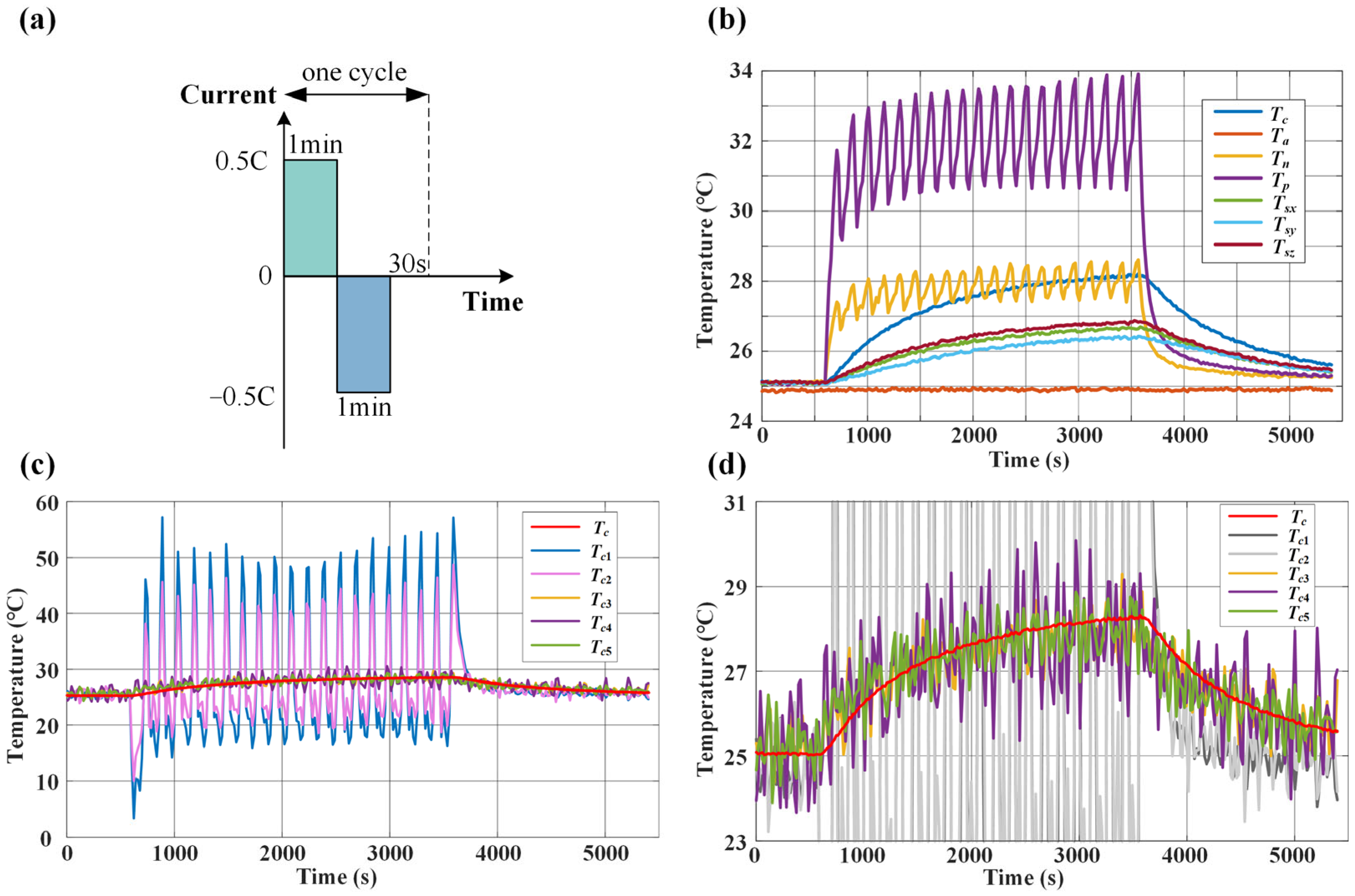
The specific experimental steps are as follows: 1. Adjust the initial SOC of the battery to 50%; 2. Set the temperature chamber to 25 °C and allow it to stand for 2 h to equilibrate the battery’s internal and external temperatures; 3. Conduct a 0.5C pulse charge–discharge experiment on the battery, where the battery is charged for 1 min, discharged for 1 min, and then rested for 30 s. This sequence is repeated for 10 cycles; 4. Record the data, using a data logger to record temperature data at different points and a charge–discharge cycler to record electrical data, maintaining a constant data sampling period. The experimental profile is shown in Figure 9a.
The least-squares parameter identification procedure proceeds as follows. First, each governing equation in Equations (4)–(8) is discretized using a first-order backward-difference scheme for the time derivative dT/dt, with the sampling period (approximately 1 s, consistent with the data logger configuration) chosen to be much smaller than the smallest expected thermal time constant of the system. After discretization, each equation becomes linear in the unknown parameter combinations (Ri Ci pairs), enabling direct closed-form least-squares solution. For each thermal branch i, the parameters are obtained by minimizing the sum of squared residuals between the branch-predicted core temperature Tci(k) and the measured ground-truth core temperature Tc(k):
J i = k = 1 N ( T c i ( k ) T c ( k ) ) 2
where N is the number of sampled time steps within the pulse identification window. The branches are identified independently. The resulting identification RMSEs (Table 2) quantify the goodness-of-fit of each branch and directly inform the subsequent model simplification: branches with large identification RMSE values (Tc1 from positive tab: 18.97 °C; Tc2 from negative tab: 14.22 °C) are pruned in favor of low-RMSE surface-derived branches (Tc3, Tc5 from x and z directions, both below 0.6 °C), leading to the final 4-input simplified model (Equation (17)).
Following the experimental steps outlined above and based on the formulated physical model Formulas (4)–(9) in Section 2, the least squares method is used to identify each set of thermal circuit parameters. The raw data from the pulse charge–discharge experiment and the parameter identification results are shown in Figure 9b–d. In Figure 9c,d and Table 2, Tc1 to Tc5 represent the internal temperature estimations obtained from the least squares identification results of the corresponding physical Equations (4)–(8). Table 3 presents the parameter identification results for Equations (4)–(8).
Specifically, Tc1 and Tc2 reflect the estimated internal temperature values obtained through the battery’s positive and negative terminal temperatures and the corresponding thermal circuit calculations. In Table 3, RpCp and RcpCp, and RnCn and RcnCn are the parameters of the transfer equations from the surface temperature of the positive and negative electrode tabs to the internal temperature of the battery, respectively. Their identification results and internal temperature estimates are different from the surface temperatures in the x, y, and z directions of the battery surface. The appearance of negative values in the identification results is primarily due to the metallic materials of the positive and negative electrode tabs, which have small specific heat capacities and are in direct contact with the air. This leads to a very low thermal resistance to the environment. Consequently, the temperature rises rapidly during charging and discharging and drops rapidly during rest. Therefore, the model constructed in Section 2 can be optimized by not considering the heat conduction effect of the battery electrode tab temperatures Tn and Tp on the internal temperature.
Tc4 reflects the internal temperature obtained from the Y-axis surface temperature and the corresponding thermal circuit calculation. Rsy1Csy and Rsy2Csy represent the transfer equation parameters from the thermal branch of the Y-direction surface temperature to the battery internal temperature. Theoretically, the Y-axis surface measurement point is farthest from the geometric center of the winding core and therefore belongs to a non-primary heat conduction path. From a data perspective, the differences in identified time constants corroborates the hysteresis of its thermal response and its weak correlation with the core temperature. This convergence of theoretical analysis and experimental validation indicates that retaining the Y-axis input contributes marginally to accuracy improvement while substantially increasing both the sequence length and computational burden on the edge microprocessor. Consequently, the final model is optimized to retain only the X- and Z-axis surface temperatures and ambient temperature as inputs.
Based on the above analysis and the parameter identification results provided in Table 2 and Table 3, the model input parameters can be further simplified, and the number of temperature measurement points in practical applications can be reduced. The model parameters are ultimately simplified to the battery surface temperatures Tx and Tz along the x-axis and z-axis directions, the ambient temperature Ta, and the battery heat generation Qc. Simultaneously, the constraints of the physical model are optimized and modified as follows:
C cx d ( T sx T a ) d t = T c T sx R cx1 + T a T sx R cx2 C cz d ( T sz T a ) d t = T c T sz R cz1 + T a T sz R cz2 C c d ( T c T a ) d t = T sx T c R cx1 + T sz T c R cz1 + Q c

3.3. Training and Offline Validation of the ThermaPhysLite Model

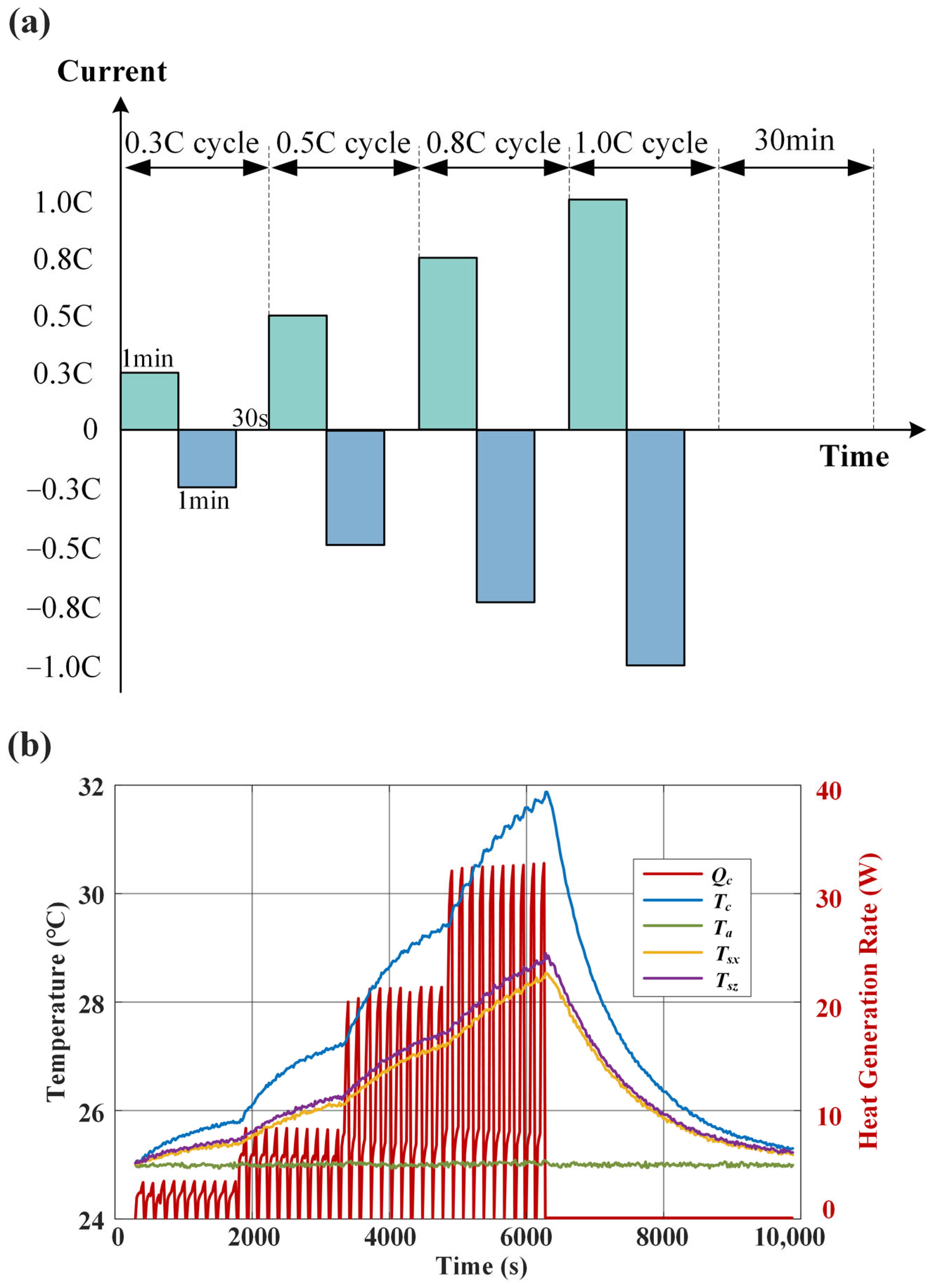
Pulsed charge–discharge experiments are designed to excite sufficient thermal dynamics for parameter identification while maintaining an approximately constant SOC. The short pulse duration ensures that SOC variations within the identification window are negligible, thereby isolating the thermal response from electrochemical state changes. The variable current pulse charge–discharge experimental condition for the battery is shown in Figure 10a. The battery is sequentially subjected to 0.3C, 0.5C, 0.8C, and 1.0C pulse charge–discharge, where the battery is charged for 1 min, discharged for 1 min, and then rested for 30 s; the pulse condition at each current is repeated for 10 cycles, and after completing the pulse condition at all currents, it is allowed to stand for 30 min.
The obtained training set data are shown in Figure 10b. It can be seen from the figure that within the normal operating temperature range, the internal temperature rise in the battery reaches approximately 7 °C, the maximum surface temperature rise is approximately 4 °C, and the maximum temperature difference between the battery surface temperature and the internal temperature can reach approximately 3 °C, accounting for 75% of the surface temperature rise. These results fully demonstrate the importance of internal temperature estimation for battery state assessment. The training set data are divided according to the data format required by ThermaPhysLite. Then, the identification results of the thermal circuit parameters and the sampling period are analyzed. The selected sequence length must satisfy the condition that the overall time scale is greater than the maximum time constant of any branch in the thermal circuit model. The proposed ThermaPhysLite is designed as an internal temperature estimation model that maps external observable variables (Ta, Tsx, Tsz, Qc) over a historical context window of length 64 to the internal temperature Tc at the same time instant. The internal temperature Tc does not appear in the model input; the historical window is employed to provide thermal dynamics context (e.g., capturing the surface-to-core heat conduction lag), rather than to infer future values from past values of the target variable. This estimation paradigm structurally precludes the chronological data leakage concern that arises in forecasting tasks.
After sliding-window construction from the training experiment data (Figure 10), 70% of the resulting sequences are used for parameter optimization, while the remaining 30% for monitoring the validation loss during training (Figure 11). Additionally, the MS-TCN architecture employs causal convolutions (Equation (10)), which structurally preserve chronological causality at the architectural level. The principal evaluation of model generalization is conducted on three independently acquired experiments (Testing Conditions I-III, also described in this section), which were acquired separately under operating profiles distinct from those of the training experiment.
The hyperparameter settings for the training process are shown in Table 4.
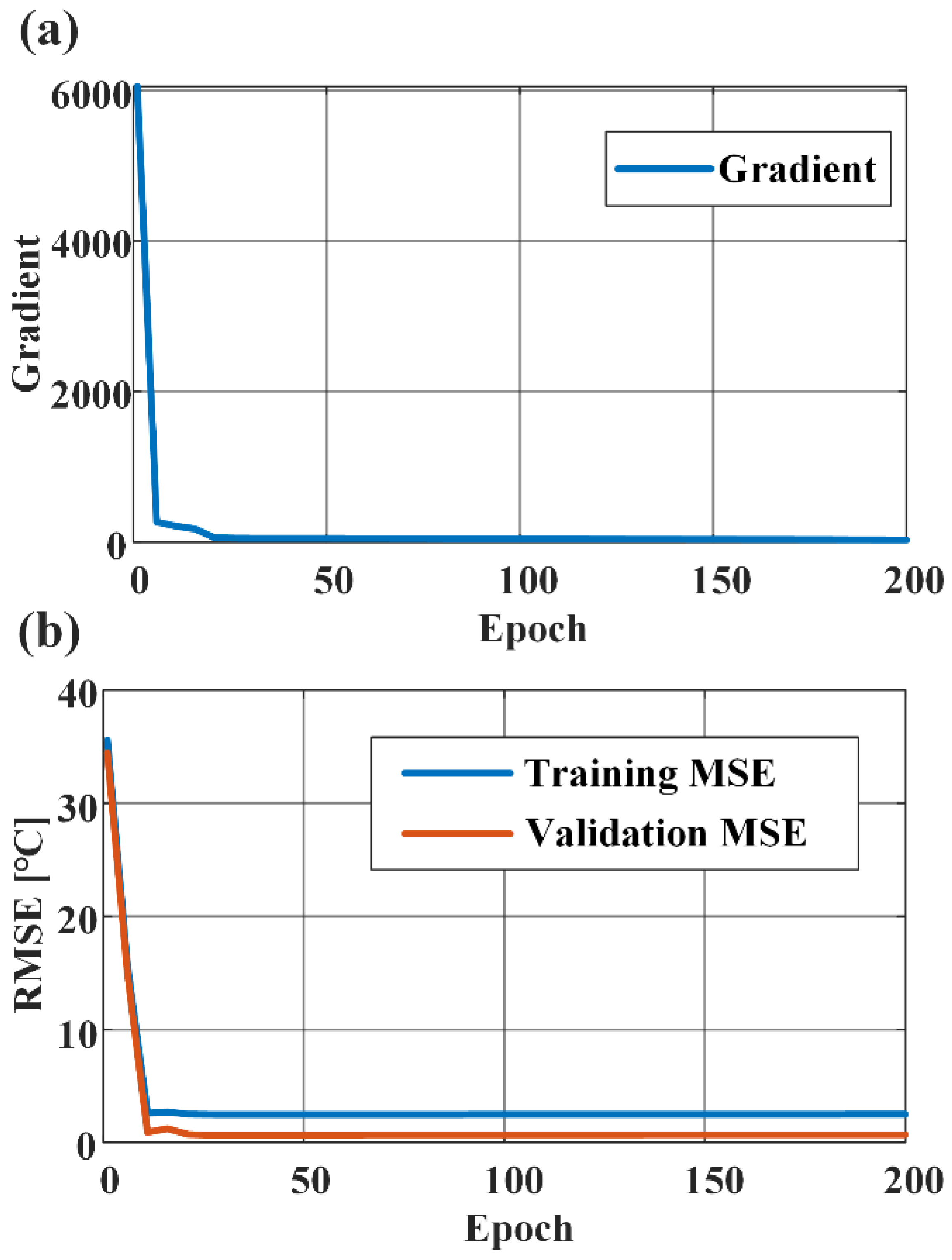
ThermaPhysLite was implemented and trained using the Tensorflow library in Python 3.7.0. The training dynamics of ThermaPhysLite are shown in Figure 11, which presents the gradient changes and RMSE values for the training and validation sets.
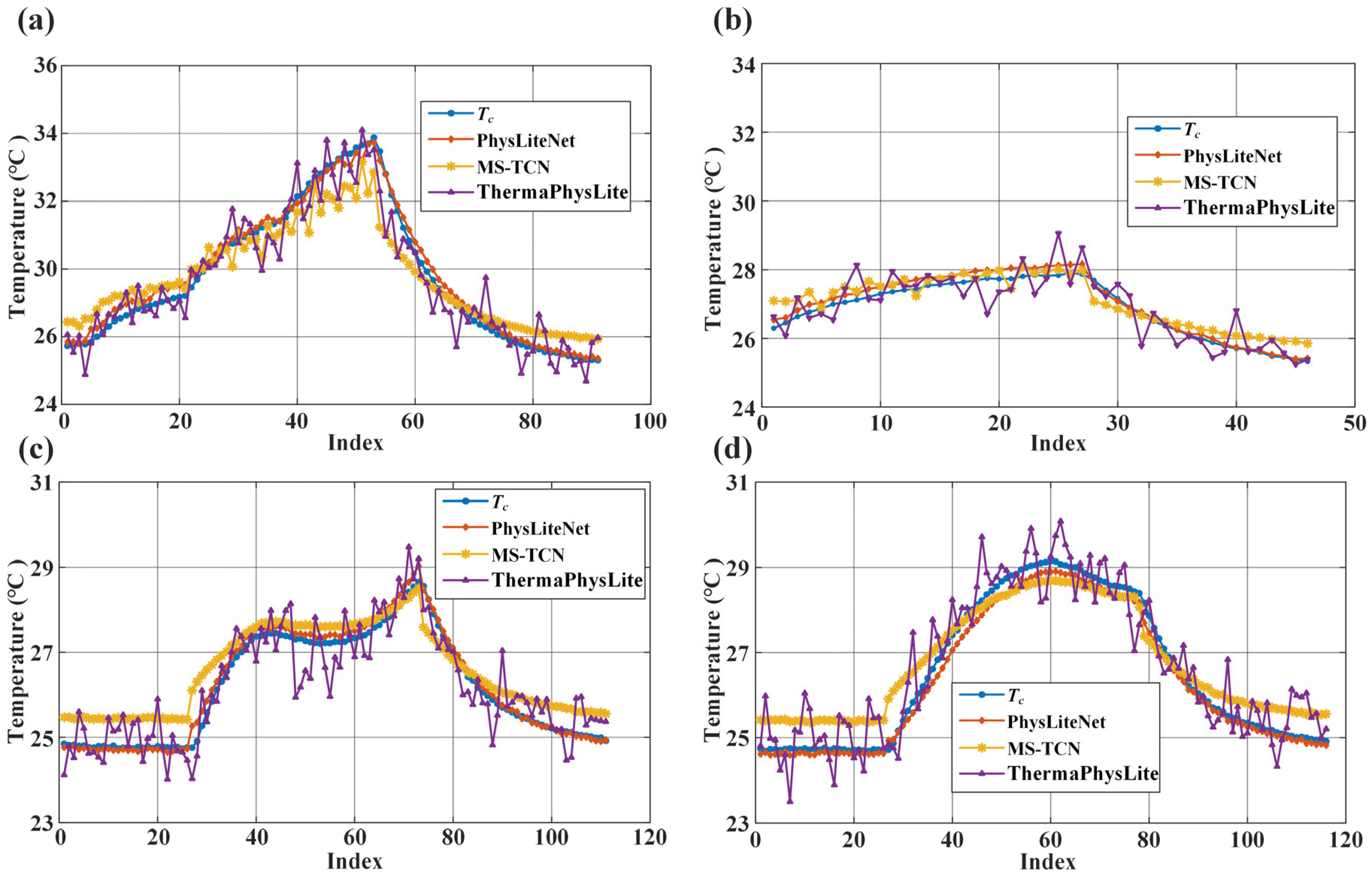
The training results are depicted in Figure 12a. We trained and evaluated the proposed ThermaPhysLite, the MS-TCN, and the physics-based model formulated from Equation (17). The performance of each model was assessed by calculating the RMSE and the maximum absolute error between the predicted internal temperature and the actual internal temperature.
To validate the generalization capability and accuracy of the proposed model, a series of experiments was designed to test the model under various operating conditions. The specific testing conditions are detailed below:
Testing Condition I: The battery underwent pulsed charge–discharge cycles at a constant ambient temperature of 25 °C. Each cycle consisted of one-minute charging at 0.6C, followed by a one-minute discharge at 0.6C. This sequence was repeated for 10 cycles, followed by a 30 min rest period.
Testing Condition II: The battery was subjected to constant current discharge at 0.5C at a constant ambient temperature of 25 °C. The battery was discharged from 100% SOC to 0% SOC.
Testing Condition III: The battery was subjected to constant current charging at 0.5C at a constant ambient temperature of 25 °C. The battery was charged from 0% SOC to 100% SOC.
Based on the experimental conditions described above, the collected data were subjected to offline analysis, and the results of the three sets of test conditions are shown in Figure 12b–d.
The training and testing errors for ThermaPhysLite, the MS-TCN, and the physics-based model are summarized in Table 5 and Table 6, respectively.
These results indicate that the proposed ThermaPhysLite model offers higher accuracy than the compared methods. ThermaPhysLite consistently achieved the lowest error metrics across all testing conditions. Specifically, the RMSE values were 0.19 °C, 0.15 °C, and 0.20 °C, while the maximum absolute error values were 0.31 °C, 0.48 °C, and 0.46 °C for the three testing conditions, respectively.
Synthesizing the aforementioned offline validation results, the strengths and limitations of different modeling paradigms can be scrutinized from a methodological perspective.
Traditional physics-based methods are constrained by the static parameter assumption. Despite possessing the strongest interpretability, the fixed thermal resistance and capacitance parameters struggle to dynamically adapt to the complex non-linear electrochemical environment of the battery. Consequently, this leads to a bottleneck in inference accuracy under variable operating conditions, as evidenced by the relatively higher RMSE values.
In contrast, while the purely data-driven MS-TCN model can capture latent trends during charge–discharge processes by learning from extensive datasets, it fundamentally remains a black-box approach. Such models exhibit strong dependence on both training sample size and the representativeness of operating conditions in the training data. In practical engineering scenarios often characterized by limited high-fidelity measurements, purely data-driven models are susceptible to overfitting when encountering extreme conditions absent from the training set. These models may even generate predictions that violate fundamental thermodynamic principles, thereby lacking essential physical interpretability and safety guarantees.
However, the PINN-based approach (ThermaPhysLite) proposed in this study successfully addresses the limitations of both traditional physics-based models that rely on complex analytical solutions and data-driven methods that demand extensive training datasets. By embedding physical constraints within the neural network loss function, ThermaPhysLite constrains the optimization process to a solution space that respects thermodynamic laws. This mechanism not only substantially enhances learning efficiency in data-scarce regimes but also ensures physical consistency: physical priors guarantee the plausibility and robustness of predictions, while the neural network’s nonlinear approximation capability effectively compensates for simplifications in the physical model. This integration of physics-based constraints and data-driven flexibility demonstrates significant practical value for battery state estimation applications where reliability is critical.

4. Design and Validation of an On-Line Internal Temperature Estimation Device for Lithium-Ion Batteries

Sensorless internal temperature estimation for lithium-ion batteries, utilizing heat generation information derived from external temperature measurements and electrical signals (voltage and current), is of paramount importance for battery state estimation and proactive safety monitoring. This study aims to develop a computationally efficient model structure based on a low-complexity physical model. By incorporating a priori knowledge from the physical model, the reliance of the ThermaPhysLite model on extensive data during the training phase is mitigated. Ultimately, an online internal temperature estimation device suitable for practical engineering applications is designed and implemented on an embedded platform supporting tensor operations.
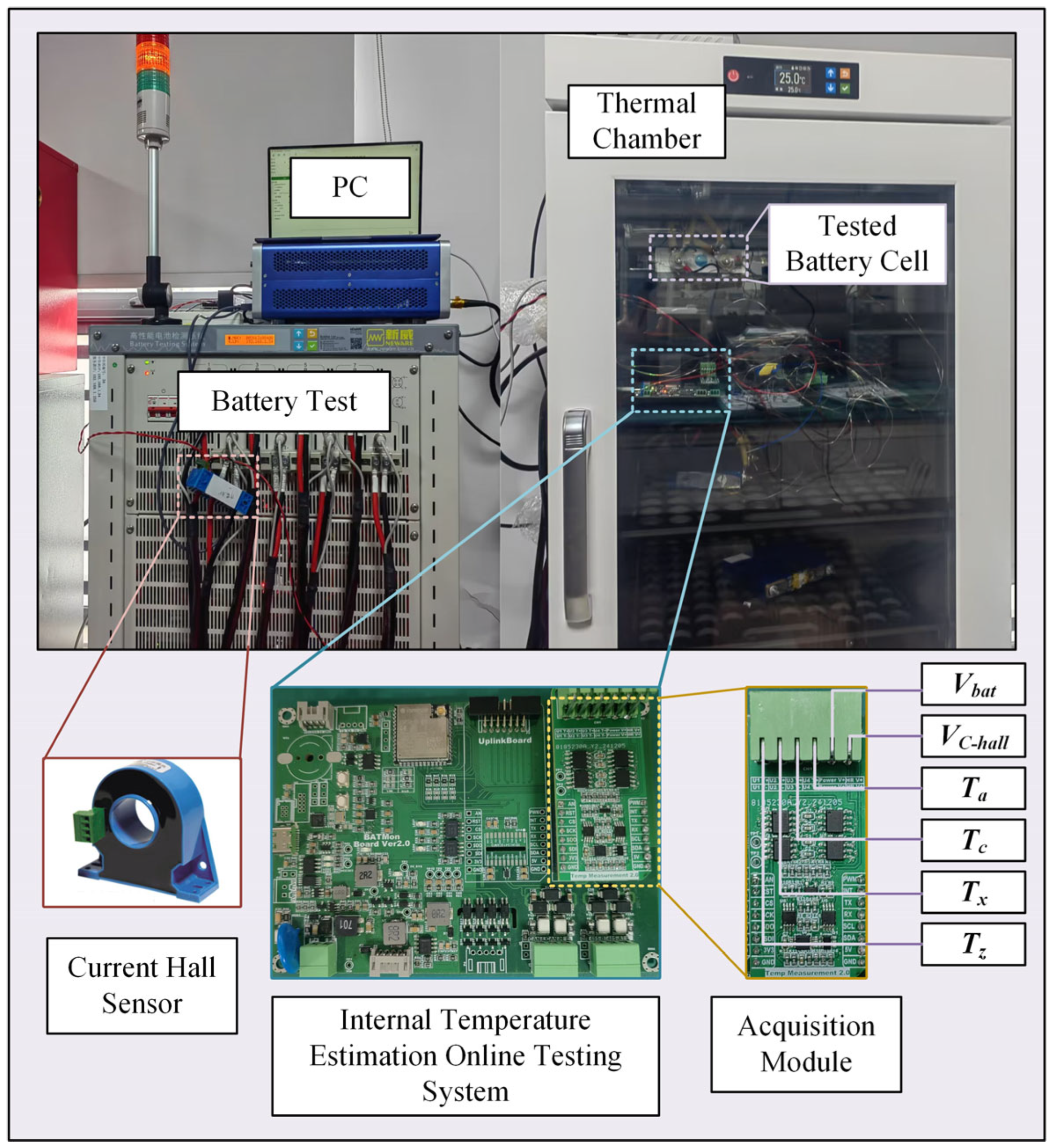
The online internal temperature estimation system designed in this study utilizes the ESP32-S3 microcontroller (Espressif Systems, Shanghai, China) as the edge computing platform, supporting TensorFlow Lite model deployment. The ESP32-S3 is a high-performance, low-power edge-class microcontroller tailored for Internet of Things (IoT) applications, featuring an integrated vector processor specifically designed to accelerate machine learning and neural network inference tasks. Furthermore, it supports machine learning frameworks such as TensorFlow Lite, enabling the seamless porting of trained models to the device. The feasibility of this deployment pipeline was preliminarily demonstrated in [26], where INT8 quantization reduced the model size to 84.29 KB with a compression ratio of 16.02×, achieving inference latency below 120 ms while retaining estimation accuracy. The overall architecture of the online experimental platform is depicted in Figure 13. Adopting a modular design approach, the system integrates standardized acquisition modules via SPI and I2C interfaces. The key hardware components are detailed in Table 7.
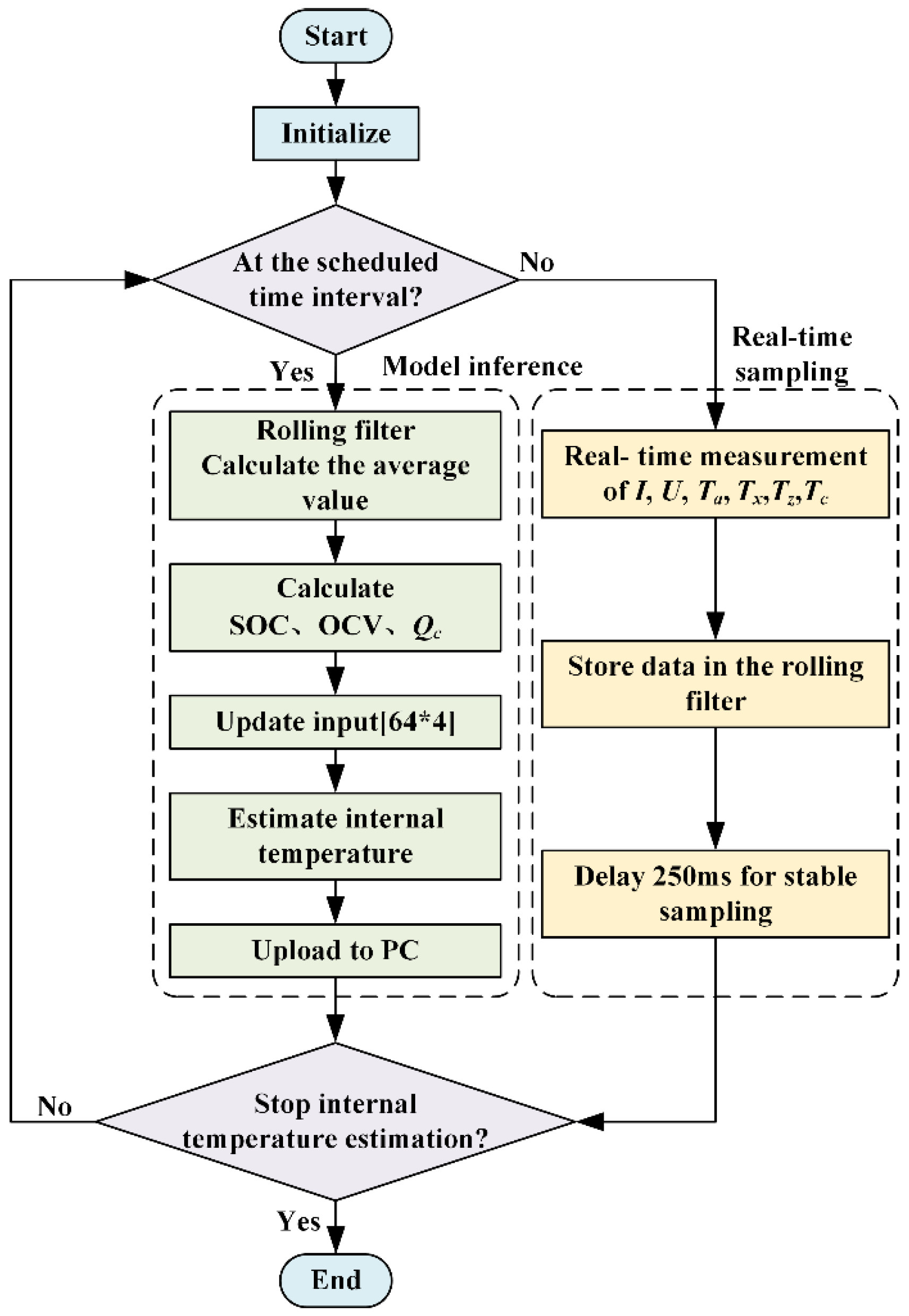
The software architecture of the system is illustrated in Figure 14 and comprises three primary modules: Initialization, Real-time Sampling, and Model Inference. Following initialization, the Real-time Sampling module operates continuously, utilizing a moving average filter to synchronously acquire five key feature variables: ambient temperature Ta, battery surface temperatures Tx, Tz, battery terminal voltage Vbat, and the current signal VC-hall. The Model Inference module is designed to be triggered at predetermined intervals. It inputs the processed feature sequence into the ThermaPhysLite model deployed on the MCU, and the calculated internal temperature estimate Tpred is output to the host computer in real time for online state estimation.
To validate the engineering applicability of the proposed model following its transfer to the embedded platform, online experiments were designed to verify the generalization capability and accuracy of the internal temperature estimation system. The designed experimental conditions are as follows:
Test Condition I: At a constant temperature of 25 °C, the battery was subjected to pulsed charge–discharge currents of 0.4C and 0.5C (i.e., charging for 1 min, discharging for 1 min and then resting for 30 s) for 20 cycles. The current was then changed, and the pulsed cycling was repeated, followed by a 30 min rest period.
Test Condition II: The battery was discharged at a constant current of 0.5C from 90% SOC to 10% SOC while maintaining a constant ambient temperature of 25 °C.
Test Condition III: The battery was charged at a constant current of 0.5C from 10% SOC to 90% SOC while maintaining a constant ambient temperature of 25 °C.
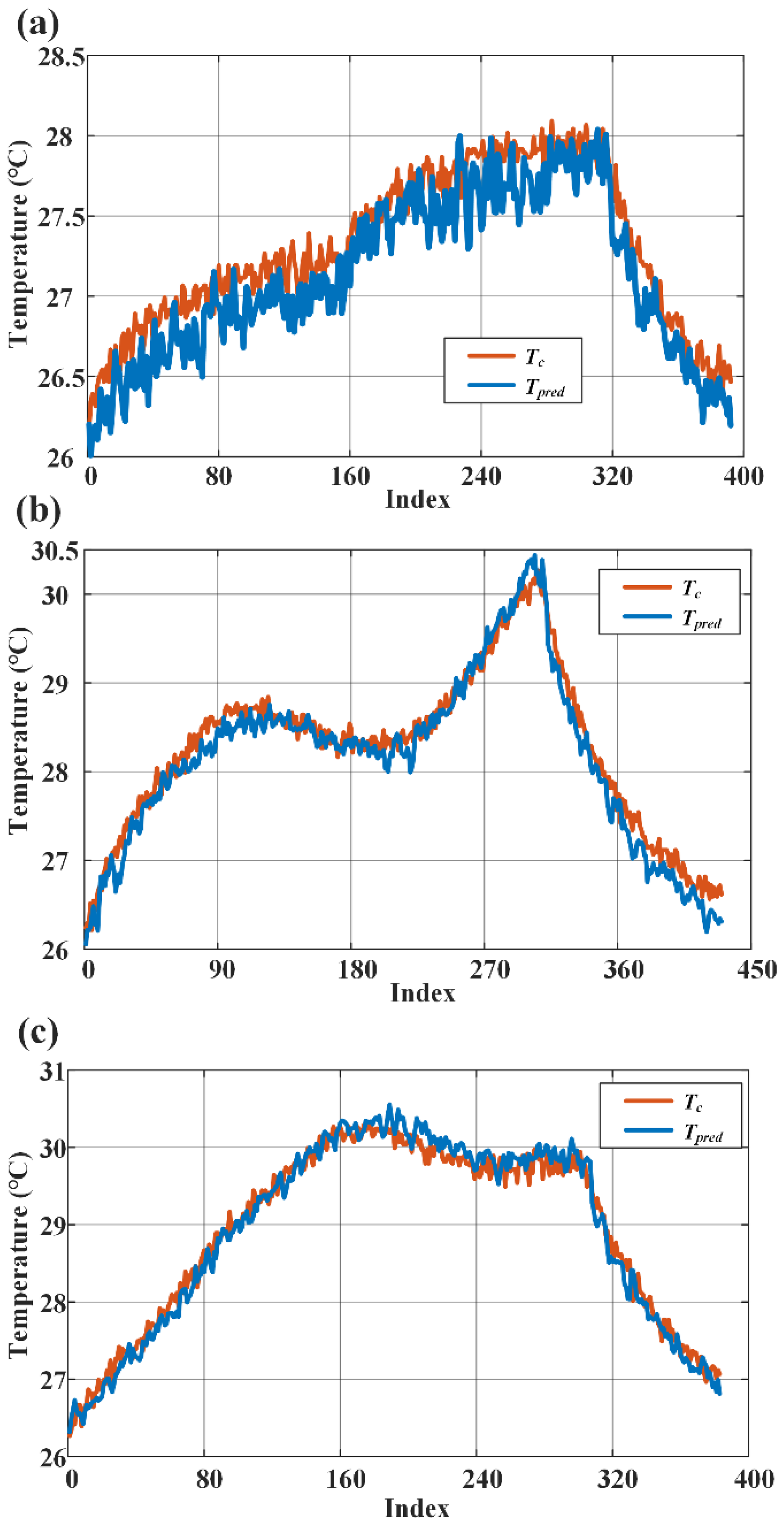
During the experiments, the actual internal temperature of the lithium-ion battery (Tc) and the estimated internal temperature Tpred obtained from the online testing system were collected. The results for each testing condition are depicted in Figure 15. It is noted that these online test conditions are consistent with those reported in [26], where a prototype system based on the same embedded platform was validated; the present work provides a more complete experimental characterization alongside the systematic offline validation in Section 3.
The RMSE of the ThermaPhysLite model for the overall test set is shown in Table 8.
In summary, the ThermaPhysLite model proposed in this study demonstrates high accuracy, even when running online. The RMSE for the three test sets were only 0.24 °C, 0.20 °C, and 0.17 °C. The average processing times for single-cell internal temperature estimation under different test conditions is 119.44 ms, 119.67 ms, and 119.40 ms, respectively. Based on the online test results in Table 8 and the hierarchical architecture characteristics of large-scale energy storage stations, the engineering application value of this method is discussed in depth below from three dimensions: edge computing adaptability, real-time response capability, and cloud–edge collaboration architecture fusion.
First, the experimental results verify the high fidelity and feasibility of the proposed method on resource-constrained edge devices. Although ThermaPhysLite is deployed on the computationally limited ESP32-S3 embedded platform, its online estimation RMSE under various dynamic conditions remains within the range of 0.17~0.24 °C. These empirical data strongly support the effectiveness of the model simplification strategy in Section 2—namely, retaining the core thermodynamic characteristics of the model while significantly reducing computational complexity through physical model dimensionality reduction and MS-TCN non-linear compensation. This indicates that the algorithm possesses the engineering potential for large-scale embedded deployment on low-cost BMS slave modules, overcoming the computational bottleneck that prevents traditional high-order physical models from landing at the edge.
Second, addressing the real-time requirements of large-scale energy storage systems, the inference latency of this paper is within the safe threshold permitted by engineering standards. Empirical data shows that the single-cell inference time is approximately 120 ms. Considering the Distributed Architecture commonly adopted by commercial storage BMS, where a single slave microcontroller typically manages 12 to 24 battery cells in series, it is estimated that a full temperature scan of a module takes about 1.44 s. Given the significant Large Thermal Inertia characteristic of the lithium-ion battery temperature field, as a slow-varying state quantity, a second-level refresh frequency is sufficient to meet the thermal management system’s need to capture early signs of thermal runaway. Furthermore, addressing potentially stricter latency constraints in the future, Model Quantization and Pruning techniques [37] can serve as technical paths for subsequent optimization, further compressing model size and increasing inference speed with minimal sacrifice in precision.
To make the algorithm scheduling more concrete in the context of actual BMS operation, we propose a time-triggered serial inference scheme suitable for integration into the distributed BMS architecture. At each refresh period Trefresh, the slave microcontroller sequentially performs ThermaPhysLite inference on its 12–24 managed cells: for each cell, the already-sampled inputs (Ta, Tsx, Tsz, and the Bernardi-equation-derived Qc from the existing voltage/current sampling) are fed into the deployed model, and the estimated internal temperature Tc is uploaded to the master BMS via standard SPI/CAN interfaces. ThermaPhysLite therefore does not replace the high-frequency voltage/current/surface-temperature sampling routines of mainstream BMSs—it adds an internal temperature-estimation layer on top of the existing data pipeline.
Based on the measured per-cell inference latency (120 ms), the theoretical full-module scan rate for a 12-cell module is approximately 1.44 s. However, taking into account practical engineering overhead—including data acquisition synchronization, communication latency on the SPI/CAN buses, computational buffering, and BMS task scheduling—a tentative engineering-oriented refresh period on the order of 3–5 s at the module level is suggested for practical deployment. This proposed refresh period remains well within the internal data refresh rate envelope (≤20 s) recommended for high-energy BESS applications in international BMS standards [38], leaving substantial margin for additional system-level overhead. The corresponding comparison is summarized in Table 9.
Notably, for millisecond-scale fault protection (e.g., immediate response to short-circuit events), conventional hardware-level threshold protection on surface temperature remains the primary mechanism; ThermaPhysLite serves a complementary role by providing continuous internal temperature estimation for thermal management and early-stage thermal-anomaly detection. We emphasize that the scheduling scheme described above is offered as a proposed engineering plan derived from our algorithmic measurements combined with general BMS engineering considerations, rather than a fully implemented BMS-level system; comprehensive system-level integration is identified as an important direction for follow-up work (Section 5).
Building upon the proposed scheduling scheme, the scaling of ThermaPhysLite from cell-level to module/pack-level follows the standard hierarchical BMS architecture along three dimensions. First, at the module level, the 120 ms single-cell inference time translates to the module-level scan times discussed above. Second, at the pack level, the cell-level temperature estimates from multiple slave microcontrollers can be aggregated by a master BMS controller, providing pack-level thermal distribution information for system-level decision-making such as cell balancing, fault detection, and thermal-management coordination. This hierarchical aggregation pattern aligns with standard BESS BMS designs. Third, it should be noted, however, that the current cell-level model does not explicitly account for inter-cell thermal crosstalk (e.g., heat conduction through busbars, shared cooling-plate effects); for tightly packed module configurations with significant inter-cell temperature non-uniformity, a module-level model incorporating thermal coupling would be required, which is designated as future work (Section 5).
Furthermore, this method effectively enables a cloud–edge collaborative architecture for modern energy storage management systems. Traditional monitoring systems in energy storage stations are constrained by vertically layered communication structures, where long-distance data transmission between the EMS and field devices introduces significant latency, hindering rapid responses to millisecond-scale thermal safety events. The edge deployment capability of ThermaPhysLite addresses this critical safety gap by enabling low-latency onsite temperature estimation and fault detection at the BMS edge layer, it ensures operational safety at short timescales, while computationally intensive tasks such as fleet-level data analytics and SOH assessment are offloaded to cloud infrastructure. This hierarchical task allocation strategy not only resolves the inherent trade-off between communication bandwidth and real-time performance but also provides a practical framework for developing high-safety, high-efficiency energy storage systems in modern power grids.

5. Summary

5.1. Summary of Findings

Recognizing the critical influence of battery temperature on performance and safety, this paper proposes ThermaPhysLite, a lightweight physics-informed neural network (PINN) framework for online internal temperature estimation of large-format prismatic Li-ion cells in stationary energy storage applications. The proposed framework integrates a simplified electro–thermal coupled model—a lumped-parameter thermal circuit coupled with the Bernardi heat generation equation—into a multi-scale temporal convolutional network (MS-TCN) through the PINN training paradigm. The physical model is systematically simplified through structural reduction and data-driven input pruning to enable edge deployment, while the embedded physics-informed loss term preserves physical consistency in the learned mapping.
Offline validation under three distinct operating conditions demonstrates RMSE values below 0.20 °C and maximum absolute errors below 0.48 °C. The framework is further deployed on an ESP32-S3 embedded platform via TensorFlow Lite, with the INT8-quantized model size reduced to 84.29 KB (16× compression). Online experiments under three additional independent testing conditions confirm RMSE values of 0.17–0.24 °C with a single-cell inference latency of approximately 120 ms, validating the engineering viability of the proposed approach for resource-constrained BMS deployment.

5.2. Engineering Significance

Beyond the algorithmic contribution, ThermaPhysLite addresses three key engineering needs in stationary BESS applications. First, the lightweight design enables internal temperature estimation directly on low-cost BMS slave microcontrollers, overcoming the computational bottleneck that prevents traditional high-order physical models or unconstrained deep learning models from being deployed at the edge. Second, the proposed time-triggered serial inference scheme (Section 4) is compatible with the distributed BMS architecture commonly used in commercial BESS, with an engineering-oriented refresh period of 3–5 s per module that is consistent with mainstream LFP-BMS practices and within the international BMS standard envelope for BESS applications. Third, the approach naturally fits into the cloud–edge collaborative paradigm: low-latency continuous internal temperature estimation at the edge can be complemented by cloud-side analytics for fleet-level health assessment and periodic model updates, enabling a hierarchical, safe, and efficient BESS management framework.

5.3. Limitations

Despite the demonstrated effectiveness of the proposed method, we honestly acknowledge several limitations bounding the current scope of this work:
(1)
Operating temperature envelope: The current experimental validation was conducted at a controlled ambient temperature of 25 °C, representative of the typical operational window (15–35 °C) of thermally controlled BESS [7,8]. Within this thermally controlled envelope, both the constant-parameter assumption and the chosen validation conditions were well-justified for the intended engineering application. Extension to scenarios with significant ambient temperature drift (e.g., automotive applications spanning −20 °C to 50 °C) lies outside the scope of this work.
(2)
Aging-related boundary: The current validation was conducted exclusively on fresh cells. The MS-TCN residual-learning mechanism was designed to compensate for short-term parameter variations within the training distribution; long-term parameter drift caused by battery aging—particularly when SOH degrades beyond the typical BESS operational window (the standard EOL criterion of SOH = 80%)—lies outside the inherent compensation capability of the current model. While existing studies suggest that operationally relevant aging-induced changes to thermal dissipation parameters remain within a moderate range within this window, this assumption was not experimentally verified in the present work.
(3)
Applicability boundary—chemistry, geometry, and scale: The methodology has been developed and validated on large-format prismatic LFP cells. Extension to other Li-ion chemistries (e.g., NMC, NCA) requires re-acquisition of chemistry-specific OCV-SOC and dOCV/dT characteristics, re-identification of thermal circuit parameters, and re-training of the MS-TCN. Extension to cylindrical or pouch form factors would require corresponding adaptation of the thermal circuit topology. Furthermore, the current cell-level model does not explicitly account for inter-cell thermal crosstalk (e.g., conduction through busbars, shared cooling-plate effects) in tightly packed modules.
(4)
Hardware instrumentation considerations: The current ground-truth acquisition employs invasive side-drilling thermocouple embedding on cells of the same batch, which is suitable for offline model development and validation but is not practical for in-field BESS deployment. Future versions of the framework would benefit from less invasive sensing techniques.

5.4. Future Work

Building upon the current work, several concrete directions are identified for future research:
(1)
Full-lifecycle adaptation via cloud–edge collaboration: To address the aging challenge in a manner consistent with the engineering deployment scenario, we propose extending the present framework with a periodic update mechanism that exploits the cloud–edge collaborative architecture described in Section 4. The proposed pathway consists of: (a) periodic online parameter re-identification on representative cells during scheduled BESS maintenance windows; (b) cloud-side model re-training with the updated parameters and edge re-deployment of the new model; and (c) introducing SOH as an auxiliary input variable into the MS-TCN to enable learning of SOH-dependent residual patterns. Recent aging-integrated battery temperature estimation work [39] supports the feasibility of this direction.
(2)
Module-level thermal management extension: Extending the research object from single cells to realistic module environments, focusing on liquid-cooling-plate heat exchange boundaries and thermal crosstalk effects between adjacent batteries, to construct a system-level temperature estimation model closer to actual energy storage station scenarios.
(3)
System-level BMS integration: While the present work has demonstrated the algorithm-level feasibility of ThermaPhysLite on a representative embedded platform, comprehensive system-level integration into commercial BMS architectures—including detailed task scheduling, communication protocol optimization, and field validation in actual BESS deployments—remains an important engineering direction for follow-up work.
(4)
Comprehensive deployment metrics benchmarking: Systematic measurement and reporting of runtime memory footprint, peak heap usage, and power consumption under inference on the embedded platform, following emerging benchmarking practices in the embedded machine learning community.
(5)
Deeper interpretability analysis: While the proposed hybrid framework provides physical consistency through embedded thermodynamic constraints, a more comprehensive interpretability analysis—including feature attribution analysis on MS-TCN inputs, sensitivity analysis of the physics-informed loss term, and visualization of the learned residual patterns—remains a valuable direction for future research. Such analyses would provide deeper insight into how the data-driven and physics-based components interact, supporting more transparent and trustworthy deployment in safety-critical BESS applications.
(6)
Advanced sensing technologies: Exploring integration of wireless passive sensors or fiber-optic sensors with battery manufacturing processes to obtain more precise internal temperature field distributions, thereby further perfecting the validation framework.

Supplementary Materials

The following supporting information can be downloaded at: https://www.mdpi.com/article/10.3390/batteries12060189/s1.

Author Contributions

Z.L.: conceptualization, methodology, software, validation, formal analysis, data curation, visualization, writing—original draft. Y.W.: supervision, project administration, funding acquisition, resources, writing—review and editing. P.G.: supervision, resources, funding acquisition. H.L.: methodology, software, validation, investigation, data curation. T.C.: supervision, project administration, writing—review and editing. G.S.: investigation, data curation. Z.W.: investigation. Y.M.: resources, writing—review and editing. All authors have read and agreed to the published version of the manuscript.

Funding

This work was supported by the Key Laboratory of Electrochemical Energy Safety, Ministry of Emergency Management (No. EES2025KF07).

Data Availability Statement

A representative dataset corresponding to Testing Condition III (online deployment validation) is provided as Supplementary Information (including the complete data pipeline from raw electrical signals through to the ThermaPhysLite predictions, accompanied by an README and a CC BY 4.0 license). The complete data supporting the findings of this study are available from the corresponding author upon reasonable request.

Conflicts of Interest

Authors Yan Wang, Ping Gao and Yuxin Meng were employed by the company XYZ Storage Technology Co., Ltd. The remaining authors declare that the research was conducted in the absence of any commercial or financial relationships that could be construed as potential conflicts of interest.

References

  1. Zhang, S.S.; Xu, K.; Jow, T.R. The low temperature performance of Li-ion batteries. J. Power Sources 2003, 115, 137–140. [Google Scholar] [CrossRef]
  2. Chen, Y.; Xiao, R.; Cui, Y.; Chen, M. Research review on early warning and suppression technology of Lithium-ion battery fire in energy storage power station. Chin. J. Electr. Eng. 2022, 17, 72–87. [Google Scholar]
  3. Liu, K.; Hu, X.; Wei, Z.; Li, Y.; Jiang, Y. Modified Gaussian process regression models for cyclic capacity prediction of lithium-ion batteries. IEEE Trans. Transp. Electrif. 2019, 5, 1225–1236. [Google Scholar] [CrossRef]
  4. Divakaran, A.M.; Minakshi, M.; Bahri, P.A.; Paul, S.; Kumari, P.; Divakaran, A.M.; Manjunatha, K.N. Rational design on materials for developing next generation lithium-ion secondary battery. Prog. Solid State Chem. 2021, 62, 100298. [Google Scholar] [CrossRef]
  5. Zhao, R.; Liu, J.; Gu, J.; Zhai, L.; Ma, F. Experimental study of a direct evaporative cooling approach for Li-ion battery thermal management. Int. J. Energy Res. 2020, 44, 6660–6673. [Google Scholar] [CrossRef]
  6. Parhizi, M.; Ahmed, M.B.; Jain, A. Determination of the core temperature of a Li-ion cell during thermal runaway. J. Power Sources 2017, 370, 27–35. [Google Scholar] [CrossRef]
  7. Mdachi, N.K.; Choong-koo, C. Comparative Review of Thermal Management Systems for BESS. Batteries 2024, 10, 224. [Google Scholar] [CrossRef]
  8. Alawi, A.; Saeed, A.; Sharqawy, M.H.; Al Janaideh, M. A Comprehensive Review of Thermal Management Challenges and Safety Considerations in Lithium-Ion Batteries for Electric Vehicles. Batteries 2025, 11, 275. [Google Scholar] [CrossRef]
  9. Xiong, R.; Li, X.G. Battery internal temperature estimation method through double extended Kalman filtering algorithm. Chin. J. Mech. Eng. 2020, 56, 146–151. [Google Scholar]
  10. Guo, Z.; Xu, J.; Xu, Z.; Mubashir, M.; Wang, H.; Mei, X. A three-heat-source electro-thermal coupled model for fast estimation of the temperature distribution of a lithium-ion battery cell. IEEE Trans. Transp. Electrif. 2022, 8, 288–297. [Google Scholar] [CrossRef]
  11. Xie, Y.; Li, W.; Hu, X.; Lin, X.; Zhang, Y.; Dan, D.; Feng, F.; Liu, B.; Li, K. An enhanced online temperature estimation for lithium-ion batteries. IEEE Trans. Transp. Electrif. 2020, 6, 375–390. [Google Scholar] [CrossRef]
  12. Rodríguez-Iturriaga, P.; Anseán, D.; López-Villanueva, J.A.; González, M.; Rodríguez-Bolívar, S. A method for the lifetime sensorless estimation of surface and core temperature in lithium-ion batteries via online updating of electrical parameters. J. Energy Storage 2023, 58, 106260. [Google Scholar] [CrossRef]
  13. Beelen, H.; Shivakumar, K.M.; Raijmakers, L.H.J.; Donkers, M.C.F.; Bergveld, H.J. Towards impedance-based temperature estimation for Li-ion battery packs. Int. J. Energy Res. 2020, 44, 2889–2908. [Google Scholar] [CrossRef]
  14. Fan, W.; Zhang, Z.; Dong, M.; Ren, M. On-line estimation method for internal temperature of lithium-ion battery based on electrochemical impedance spectroscopy. In Proceedings of the 2021 IEEE Electrical Insulation Conference (EIC), Denver, CO, USA, 7–28 June 2021; IEEE: Piscataway, NJ, USA, 2021; pp. 247–251. [Google Scholar]
  15. Richardson, R.R.; Ireland, P.T.; Howey, D.A. Battery internal temperature estimation by combined impedance and surface temperature measurement. J. Power Sources 2014, 265, 254–261. [Google Scholar] [CrossRef]
  16. Hussein, A.A.; Fardoun, A.A. An adaptive sensorless measurement technique for internal temperature of Li-ion batteries using impedance phase spectroscopy. IEEE Trans. Ind. Appl. 2020, 56, 3043–3051. [Google Scholar] [CrossRef]
  17. Surya, S.; Samanta, A.; Marcis, V.; Williamson, S.S. Hybrid electrical circuit model and deep learning-based core temperature estimation of Lithium-ion battery cell. IEEE Trans. Transp. Electrif. 2022, 8, 3816–3824. [Google Scholar] [CrossRef]
  18. Ouyang, K.; Fan, Y.; Yazdi, M.; Peng, W. Data-driven-based internal temperature estimation for Lithium-ion battery under variant state-of-charge via electrochemical impedance spectroscopy. Energy Technol. Ger. 2022, 10, 910–919. [Google Scholar] [CrossRef]
  19. Yuan, A.; Cai, T.; Luo, H.; Song, Z.; Wei, B. Core temperature estimation of lithium-ion battery based on numerical model fusion deep learning. J. Energy Storage 2024, 102, 114148. [Google Scholar] [CrossRef]
  20. Yao, Q.; Lu, D.D.; Lei, G. A surface temperature estimation method for Lithium-ion battery using enhanced GRU-RNN. IEEE Trans. Transp. Electrif. 2023, 9, 1103–1112. [Google Scholar] [CrossRef]
  21. Li, Y.; Ma, C.; Liu, K.; Chang, L.; Zhang, C.; Duan, B. A novel joint estimation for core temperature and state of charge of lithium-ion battery based on classification approach and convolutional neural network. Energy 2024, 308, 13272. [Google Scholar] [CrossRef]
  22. Karniadakis, G.E.; Kevrekidis, I.G.; Lu, L.; Perdikaris, P.; Wang, S.; Yang, L. Physics-informed machine learning. Nat. Rev. Phys. 2021, 3, 422–440. [Google Scholar] [CrossRef]
  23. Cho, G.; Wang, M.; Kim, Y.; Kwon, J.; Su, W. A physics-informed machine learning approach for estimating Lithium-ion battery temperature. IEEE Access 2022, 10, 88117–88126. [Google Scholar] [CrossRef]
  24. Xiong, R.; Li, X.; Li, H.; Zhu, B.; Avelin, A. Neural network and physical enable one sensor to estimate the temperature for all cells in the battery pack. J. Energy Storage 2024, 80, 110387. [Google Scholar] [CrossRef]
  25. Wang, N.; Zhao, G.; Kang, Y.; Wang, W.; Chen, A.; Duan, B.; Zhang, C. Core Temperature Estimation Method for Lithium-Ion Battery Based on Long Short-Term Memory Model with Transfer Learning. IEEE J. Emerg. Sel. Top. Power Electron. 2023, 11, 201–213. [Google Scholar] [CrossRef]
  26. Liu, Z.; Tao, C.; Luo, H.; Xiong, C. An online internal temperature estimation method for lithium-ion batteries based on physics-informed neural networks and embedded deployment. In Proceedings of the 12th Frontier Academic Forum of Electrical Engineering (FAFEE2025); Lecture Notes in Electrical Engineering; Springer: Singapore, 2026; Volume 1510, pp. 97–104. [Google Scholar]
  27. Lin, X.-W.; Jiang, Y.; Yu, H.T.; Shi, M.Y.; Liu, B.; Wen, X.L.; Zhou, Z.F. A comprehensive investigation on the electrochemical and thermal inconsistencies for 280 Ah energy storage lithium-ion battery. Energy Convers. Manag. 2024, 315, 118750. [Google Scholar] [CrossRef]
  28. Xu, S.; Wang, Y.; Shao, J.; Li, J.; Yu, Q. An electrochemical-thermal coupling model for prismatic lithium-ion batteries over wide temperature range. Appl. Therm. Eng. 2022, 217, 119282. [Google Scholar] [CrossRef]
  29. Damay, N.; Forgez, C.; Bichat, M.P.; Friedrich, G. Thermal modeling of large prismatic LiFePO4/graphite battery. Coupled thermal and heat generation models for characterization and simulation. J. Power Sources 2015, 283, 37–45. [Google Scholar] [CrossRef]
  30. Samba, A.; Omar, N.; Gualous, H.; Capron, O.; Van den Bossche, P.; Van Mierlo, J. Impact of tab location on large format lithium-ion pouch cell based on fully coupled tree-dimensional electrochemical-thermal modeling. Electrochim. Acta 2014, 147, 319–329. [Google Scholar] [CrossRef]
  31. Sheng, L.; Su, L.; Zhang, H.; Fang, Y.; Xu, H.; Ye, W. An improved calorimetric method for characterizations of the specific heat and the heat generation rate in a prismatic lithium ion battery cell. Energy Convers. Manag. 2019, 180, 724–732. [Google Scholar] [CrossRef]
  32. Barsoukov, E.; Jang, J.H.; Lee, H. Thermal impedance spectroscopy for Li-ion batteries using heat-pulse response analysis. J. Power Sources 2002, 109, 313–320. [Google Scholar] [CrossRef]
  33. Wang, S.; Teng, Y.; Perdikaris, P. Understanding and mitigating gradient flow pathologies in physics-informed neural networks. SIAM J. Sci. Comput. 2021, 43, A3055–A3081. [Google Scholar] [CrossRef]
  34. Kleiner, J.; Komsiyska, L.; Elger, G.; Endisch, C. Thermal modelling of a prismatic lithium-ion cell in a battery electric vehicle environment: Influences of the experimental validation setup. Energies 2019, 13, 62. [Google Scholar] [CrossRef]
  35. Wang, T.; Tseng, K.J.; Zhao, J. Development of efficient air-cooling strategies for lithium-ion battery module based on empirical heat source model. Appl. Therm. Eng. 2015, 90, 521–529. [Google Scholar] [CrossRef]
  36. Chen, S.C.; Wan, C.C.; Wang, Y.Y. Thermal analysis of lithium-ion batteries. J. Power Sources 2005, 140, 111–124. [Google Scholar] [CrossRef]
  37. Li, J.; Zhao, Y.; Xue, Z.; Cai, Z.; Li, Q. A survey of model compression for deep neural networks. Chin. J. Eng. 2019, 41, 1229–1239. [Google Scholar] [CrossRef]
  38. Tadoum, D.D.; Berger, F.; Krause, F.; Wasylowski, D.; Ringbeck, F.; Li, W.; Sauer, D.U. Standards and Regulations for Battery Management Systems in Germany: Review and Improvement Potentials. Glob. Chall. 2025, 9, e00129. [Google Scholar] [CrossRef]
  39. Jia, Y.; Brancato, L.; Giglio, M.; Cadini, F. Online core temperature estimation for lithium-ion batteries via an aging-integrated ECM-1D coupled model-based algorithm. Batteries 2025, 11, 160. [Google Scholar] [CrossRef]
Figure 3. First-order equivalent circuit model of the prismatic battery.
Batteries 12 00189 g003
Figure 4. Architectures of the internal temperature estimation networks: (a) Network Architecture I (Standard TCN); (b) Network Architecture II (MS-TCN with multi-scale design). In (a), the orange short blocks on the left represent the input feature sequences (Input Features a to n) arranged along the time-series dimension, as indicated by the thick black arrow at the top; the three purple bars in the first dashed box denote the Fully Connected Mapping layer that fuses all features at each time instant; the orange blocks and the subsequent orange elongated block in the second dashed box denote the Standard TCN, which performs temporal convolution on the fused feature sequence; and the green dot on the right represents the output node, corresponding to the estimated internal temperature. In (b), the orange long bars on the left represent the input feature sequences (Input Features a to n) arranged along the time-series dimension; the orange elongated blocks and the four orange short blocks in the first dashed box denote the MS-TCN, in which multiple convolutional branches with different kernel sizes and dilation factors are applied in parallel to features of different time scales; the three purple bars in the second dashed box denote the Fully Connected Mapping layer that fuses the extracted multi-scale temporal features; and the green dot on the right represents the output node, corresponding to the estimated internal temperature. Dark green arrows in both subfigures indicate the data-flow direction between layers.
Batteries 12 00189 g004
Figure 5. ThermaPhysLite network architecture and training diagram. The structure enclosed in the purple dashed frame on the (upper left) corresponds to the MS-TCN architecture detailed in Figure 4b.
Batteries 12 00189 g005
Figure 6. Experimental platform architecture diagram.
Batteries 12 00189 g006
Figure 7. Thermocouple embedding scheme: (a) battery disassembly; (b) thermocouple embedding scheme diagram I; (c) thermocouple embedding scheme diagram II; (d) thermocouple embedding result.
Batteries 12 00189 g007
Figure 8. Parameter fitting results for heat generation calculation: (a) Fitting results of OCV and SOC; (b) Fitting results of dOCV/dT and SOC.
Batteries 12 00189 g008
Figure 9. Thermal circuit parameter identification process: (a) Experimental profile (showing a single cycle schematic, whereas the actual test repeats this sequence 10 times); (b) Raw data; (c) Parameter identification results; (d) Details of parameter identification results.
Batteries 12 00189 g009
Figure 10. Training set experimental conditions and data: (a) Schematic diagram of training set experimental conditions. Note that while only a single cycle is shown for each C-rate to illustrate the pulse pattern, the actual test repeats this charge-rest-discharge sequence 10 times at each respective C-rate (0.3C, 0.5C, 0.8C, and 1.0C). (b) Training set data.
Batteries 12 00189 g010
Figure 11. Training performance of the ThermaPhysLite: (a) Gradient curves; (b) RMSE curves for the training and validation datasets.
Batteries 12 00189 g011
Figure 12. Offline validation results of the ThermaPhysLite model: (a) Comparison of training results; (b) Validation under Testing Condition I; (c) Validation under Testing Condition II; and (d) Validation under Testing Condition III (Supplementary Materials).
Batteries 12 00189 g012
Figure 13. Hardware architecture of the online experimental platform.
Batteries 12 00189 g013
Figure 14. Software flow of the online experimental platform.
Batteries 12 00189 g014
Figure 15. Comparison of online test results: (a) Test Condition I: 0.4C and 0.5C pulse charge–discharge; (b) Test Condition II: 0.5C constant current discharge; (c) Test Condition III: 0.5C constant current charge.
Batteries 12 00189 g015
Table 2. Parameter identification results for the thermal circuit model in pulse charge-discharge experiments.
Physical EquationEstimated Internal Temperature Based on Parameter Identification ResultsRMSE of Model After Parameter Identification (°C)
C p d ( T p T a ) d t = T a T p R p + T c T p R cp Tc118.9689
C n d ( T n T a ) d t = T a T n R n + T c T n R cn Tc214.2282
C sx d ( T sx T a ) d t = T c T sx R cx1 + T a T sx R cx2 Tc30.5272
C sy d ( T sy T a ) d t = T c T sy R cy1 + T a T sy R cy2 Tc40.9981
C sz d ( T sz T a ) d t = T c T sz R cz1 + T a T sz R cz2 Tc50.5498
Table 3. Parameter identification results of the thermal circuit model in pulse charge-discharge experiment.
Thermal Path ParametersIdentification Results (s)Thermal Path ParametersIdentification Results (s)
RpCp476.09Rsx2Csx495.88
RcpCp−303.48Rsy1Csy910.13
RnCn6392.91Rsy2Csy771.34
RcnCn−639.44Rsz1Csz393.25
Rsx1Csx422.60Rsz2Csz558.91
Table 4. ThermaPhysLite hyperparameter settings.
HyperparameterSettings
Input channels4
Output channels1
Sequence length64
Kernel size[3, 5, 9]
Max epoch200
Batch size20
Dilation2
Learning rate10−4
Table 5. Training and testing RMSE (°C) for offline validation.
Physical ModelThermaPhysLiteMS-TCN
Training Set0.620.180.64
Testing Condition I (Offline Validation)0.460.190.35
Testing Condition II (Offline Validation)0.540.150.53
Testing Condition III (Offline Validation)0.600.200.52
Table 6. Training and testing maximum absolute error (°C) for offline validation.
Physical ModelThermaPhysLiteMS-TCN
Training Set1.760.361.85
Testing Condition I (Offline Validation)1.210.310.79
Testing Condition II (Offline Validation)1.360.481.40
Testing Condition III (Offline Validation)1.640.461.23
Table 7. Key hardware components of the online internal temperature estimation system.
Module NameModule FunctionsMain Parameters
Main controller chip ESP32-S3Acquires voltage, current, and temperature signals; executes the ThermaPhysLite model inference; and outputs estimation results.Frequency: 240 Hz
Dual-Core LX7 Processor
Built-in 512 KB SRAM with TCM
Current Hall Sensor CHB-100SG/5V (Beijing Yubo Co., Ltd., Beijing, China)Acquires the battery charge–discharge current and converts it to a voltage signal VC-hall.Measurement Range: ±100 A
Output Voltage Range: ±5 V
Accuracy: ±0.8% (25 °C)
ADC Chip ADS1115 (Texas Instruments, Dallas, TX, USA)Acquires the battery terminal voltage signal Vbat and the voltage signal VC-hall from the current Hall sensor and transmits these voltage signals to the ESP32-S3 via the IIC bus.Input Range: ±6.144 V
Resolution: 16 bit
K-Type Thermocouple TT-K-30-SLE (Omega Engineering, Norwalk, CT, USA)Measures temperatures at various locations on the battery and the ambient temperature.Temperature Measurement Range:
−40~260 °C
Temperature Resolution: 0.1 °C
Thermocouple Reader Chip
MAX6675 (Maxim Integrated, San Jose, CA, USA)
Acquires temperature readings from the thermocouples and transmits these temperature signals to the ESP32-S3 via the SPI bus.Temperature Measurement Range: 0~1024 °C
Temperature Resolution: 0.25 °C
Table 8. Testing RMSE (°C) for online validation.
Test ConditionsRMSE (°C)Average Processing Time for Single-Cell Internal Temperature Estimation (ms)
Online Test Condition I0.24119.44
Online Test Condition II0.20119.67
Online Test Condition III0.17119.40
Table 9. Comparison of update cycles in the proposed ThermaPhysLite scheduling scheme and mainstream BMS practices for BESS applications.
ItemUpdate Cycle/IntervalReference/Source
Voltage/current sampling (mainstream BMS)1 ms–100 msStandard AFE chip capability
Theoretical full-module scan (proposed ThermaPhysLite)1.44 s
(for 12-cell module)
This work
Internal temperature refresh (proposed ThermaPhysLite)3–5 s
(per module)
This work
Internal data refresh rate (BESS standard recommendation)≤20 s[38]
Internal data refresh rate (EV/HEV standard recommendation)≤10 s[38]
Disclaimer/Publisher’s Note: The statements, opinions and data contained in all publications are solely those of the individual author(s) and contributor(s) and not of MDPI and/or the editor(s). MDPI and/or the editor(s) disclaim responsibility for any injury to people or property resulting from any ideas, methods, instructions or products referred to in the content.