


Abstract
Lithium iron phosphate batteries have seen a recent rise in usage in electric vehicles and battery energy storage systems. For these applications, reliability is of paramount importance, influences long-term adoption and high return on investment, especially regarding battery replacement. Remaining Useful Life (RUL) prediction is at the core of avoiding unexpected failure and enabling proactive battery maintenance. Physics-based and data-driven methods have been explored by researchers, whilst Physics-Informed Neural Networks (PINNs) can combine their strengths in estimating battery RUL. This paper investigates the integration of the Gompertz function, an inherently interpretable white-box model, into Long Short-Term Memory (LSTM) networks to follow the physical laws of degradation, capture downward monotonic behavior and long-term dependencies from data resulting in Gompertz-Informed LSTMs (GILSTMs). Pure LSTMs are regarded as black box systems and critical infrastructure operators such as battery energy storage system (BESS) operators may refrain from using such systems. Gray-box models such as GILSTMs may get over this hurdle by increasing model interpretability and helping industry adopters know when they will benefit from data-driven modeling. This study explores two GILSTM architectures. The first uses an LSTM to predict Gompertz parameters, which are then converted into RUL via the inverse Gompertz equation. The second uses the inverse Gompertz equation as a verification step to cross-check the RUL values generated by the LSTM. The first type of GILSTM was constrained by both a physics loss and an inverse Gompertz layer to predict RUL while the second verified the results of an LSTM, despite that the GILSTMs failed to generalize. The first type of GILSTM achieved an average RMSE of 22.97%, while the second type achieved an average RMSE of 26.99%. The models in this paper are also benchmarked on the first 100 cycles, a current state of art for battery degradation testing. The best overall implementation was an LSTM that predicted RUL by recursively predicting SoH achieving an average RMSE per cycle of 9.18% and a 100th cycle RMSE of 17.02%. This study evaluates the trade-off between the predictive accuracy of black-box LSTMs and physical interpretability of Gompertz models. While pure LSTMs provide superior accuracy, the Gompertz parameters stabilize by 85% SoH. This 85% threshold serves as an interpretable confidence trigger, informing BESS operators when to rely on LSTM RUL forecasts.
1. Introduction
An ideal power grid can match power supply and power demand by seamlessly balancing generation and consumption of power in real time. With the global rise in the use of solar and wind sources, renewable and cheap energy is now more accessible. Unfortunately, solar and wind energy are intermittent power sources, thus cannot be ramped up and down at will to match instantaneous electricity demand and stabilize the grid. Battery energy storage systems (BESS) help wind and solar systems mitigate these issues, increasing the environmentally friendly nature of many countries’ energy grids. Moreover, use of BESS improves the financial returns of renewable energy installations and improves the reliability of electricity grids by reducing energy curtailment, reducing the System Average Interruption Duration Index (SAIDI) of electricity grids [1] and reducing dependency on diesel power generation [2,3], thus improving the overall resilience of electric grids. Issues regarding power grid reliability will be exacerbated with the installation of data centers which are very sensitive to shifts in power grid frequency and can cause catastrophic blackouts [4,5,6]. Lithium iron phosphate battery-based BESS play a crucial role in storing excess energy and dispatching it when needed, energy arbitrage and providing support to maintaining the frequency of power grids [7].
However, these batteries degrade over time and can cause unintended failures to occur if not managed properly. Knowing when to replace or derate the batteries is crucial. This paper looks at understanding lithium iron phosphate (LFP) battery lifespan by conducting a comparative study on the Gompertz model, Long Short-Term Memory networks (LSTMs) and Gompertz-Informed LSTM methods toward estimation of the battery lifespan. The paper also addresses the potential implications and the ability of the methods to be interpretable by following physical degradation laws particularly the downward monotonic behavior of LFP battery capacity degradation.
2. Background and Prior Work
This section details the technical and economic context for the research, beginning with a comparative analysis of energy storage technologies to highlight the advantages of lithium ion as a storage method. It then provides a detailed examination of the electrochemical properties and operational parameters related to LFP cells. This section builds up the necessary foundation to understand battery degradation mechanisms and the technical variables such as State of Health (SoH) and Remaining Useful Life (RUL) that are essential for the predictive modelling discussed later in this paper.
2.1. Batteries and Their Characteristics
There are over 60 types of batteries, one of which is the lithium ion battery (LiB) [8,9]. There are several chemistries within LiBs, the most prominent are lithium nickel manganese cobalt oxide (NMC), lithium nickel cobalt aluminum oxide (NCA) and lithium iron phosphate (LFP) batteries. In this paper, the focus is on LFP batteries as they have recently eclipsed NMC and NCA batteries due to lower costs per kWh, thermal stability and safety [10].
Among the different types of batteries commonly used for grid scale or consumer energy applications, the choice typically depends on key factors such as storage efficiency, energy density, lifespan, discharge duration, and peak power capacity. Table 1 outlines a detailed description of common battery types. LiBs have seen increasing adoption in small- and large-scale systems due to their growing practicability [11,12]. For instance, pumped hydro costs from USD 1700 to USD 5100 per kilowatt (on average USD 3400) while LiB systems are priced from USD 2500 to USD 3900 per kilowatt (on average USD 3200) [13] yet unlike LiB-based BESS which can be deployed almost anywhere with varying scale depending on the use case, pumped hydro tends to require locations with two adjacent areas of low and high elevation and are thus constrained by geography. In addition, pumped hydro implementations require very large capital costs, keeping pumped hydro out of reach for most people, organizations and some countries.
Table 1.
Battery and their storage capacities.
Beyond cost, LiBs offer advantages in terms of modularity and ease of development, especially in urban areas, where most electricity is used. LiB systems can be implemented at household, factory and grid levels; therefore, they are expected to play an increasingly large role in the transition to renewable, decarbonized energy systems. These advantages of LiBs would be of benefit to power grids, especially regarding reducing SAIDI, integration of wind and solar energies, massively reducing the amount of grid energy that is curtailed and playing as a substitute to expensive fossil fuel power plants.
2.2. Characteristics of LFP Batteries
Lithium iron phosphate batteries (LFPs) are a safer and a more thermally stable variant of lithium ion batteries, known for their lower risk of thermal runaway [8,9,10,11], with a thermal runaway threshold ranging from 180 to 250 °C, as seen in Table 2. LFPs typically offer a lifespan ranging from 1000 to 10,000 charge–discharge cycles, which translates to approximately 2.74 to 27.4 years when used at a rate of one cycle per day. In 2024, LFPs accounted for approximately 40% to 59% of electric vehicle (EV) battery deployments, and dominated the BESS market with an estimated 80% market share [12]. Their increasing popularity is driven by their durability, cost effectiveness, and the elimination of critical materials like cobalt and nickel, making them more sustainable and geopolitically secure for large-scale energy storage and transportation applications [12].
Table 2.
Usage-related properties of LFP batteries.
The Remaining Useful Life (RUL) of LiBs refers to the number of charge–discharge cycles a battery can undergo while still maintaining an acceptable capacity. The definition of acceptable capacity is industrially defined as about 70–80% of its nominal capacity [13]. For example, an unused LFP battery with a nominal capacity of 1100 mAh may have a RUL ranging from 1000 to 10,000 cycles, depending on the manufacturer, operating conditions and usage. With each cycle, the battery undergoes gradual degradation, causing its capacity to decrease. When the capacity drops to 770–880 mAh (70–80% of 1100 mAh), the RUL reaches zero, signaling the end of its effective service life, thus a need for replacement.
The maximum capacity that the battery can draw at any point in time, relative to its capacity when new, is known as the State of Health (SoH). SoH is typically expressed as a percentage and serves as a real-time indicator of battery aging [13]. While RUL provides a forecast of how many more cycles a battery can deliver, SoH provides a snapshot of the battery’s present condition. Usage-related properties such as those in Table 2 may inform the gradual change in SoH for LFP batteries. These two parameters, SoH and RUL, are closely related and are both critical in battery management systems (BMS) for ensuring safe operation, optimizing performance, and planning timely replacements in grid scale and consumer applications. By monitoring the usage-related properties of an LFP battery, with reference to those in Table 2, the SoH and RUL of an LFP battery can be estimated. The SoH values are fixed percentage points dependent on cycling conditions while the RUL varies greatly based on usage.
Battery users may usually be more concerned with the status of the battery within each charge–discharge cycle, the proportion of energy remaining in the battery relative to its nominal energy. This proportion of energy remaining in a battery relative to its nominal energy is referred to as the State of Charge (SoC) and is usually indicated using a battery status bar or battery indicator; the nominal energy is a result of multiplying the nominal voltage with the nominal capacity and is expressed in Watt-hours (Wh) [20]. This SoC is typically expressed as a percentage ranging from 0% (fully discharged) to 100% (fully charged). If a battery is discharged below 0% SoC or charged beyond 100% SoC, irreversible chemical reactions tend to occur, leading to accelerated degradation and a significant drop in the SoH. Therefore, battery engineers have developed charging and discharging limits to properly approximate this SoC based on usage related properties as seen in Table 2.
One method for approximating SoC that has become very common for continuously operating battery systems is the Coulomb Counting (CC) method. The method is simple, standardized and is accurate for short-term calculations [21]. The method uses the Coulomb Counting SoC estimation formula shown in Equation (1) [22,23]. Where is the initial state of charge of the battery based on open-circuit voltage or predictive means. is the nominal capacity of the battery/cell when it is new. is the battery current, is the initial time and t is the time when charging or discharging occurs. This equation simply calculates the area under the curve of current over time.
The coulomb counting equation does not directly address battery decay; thus, it can be erroneous due to long-term drift of the battery capacity from the rated capacity [21]. Enhanced coulomb counting methods have been proposed to address long-term drift [14,15,24], each of which highlights the need to include battery decay by including the shift in SoH over time as shown in Equation (2).
This improvement is the integration of SoH into the traditional coulomb counting method used for State of Charge (SoC) estimation. By accounting for the reduction in usable capacity over time can provide more accurate real-time SoC estimates. To achieve the inclusion of SoH, causes of degradation need to be well understood. Charging above the maximum charge voltage can lead to overcharging, which has been found to accelerate degradation. Discharging below the minimum discharge voltage limit can result in over-discharge, leading to irreversible chemical changes that degrade the battery’s capacity and potentially render the cell unusable. Higher speeds of discharging/charging of the cells relative to the nominal capacity (C-rate) may increase internal resistance and thermal stress, leading to faster degradation. Studies show capacity fade correlates with cycles, temperature, and depth of discharge [16]. Proper estimation of SoC is usually employed to mitigate this degradation thus extending battery life. To control degradation, modern battery systems are equipped with a battery management system (BMS) that monitors and regulates SoC ensuring safe operation. SoC estimation has a direct influence on the SoH and the RUL of the battery, SoH estimation also has a direct influence on SoC and RUL. Accurate RUL prediction is essential for ensuring the reliability, safety and efficiency of battery-powered systems such as electric vehicles and renewable energy storage.
2.3. SoH and RUL Estimation Methods
The health and lifespan of any industrial equipment is very important, so is their SoH and RUL to aid in the maintenance of good operations. A battery can be defined specifically as equipment that stores and releases electrical energy. Equipment tends to suffer wear and tear and with time need to be replaced and renewed, in the case of LiBs, degradation is caused by collection of solid electrolyte interfaces (SEI) on the graphite anodes [5,25,26,27,28,29] reducing the amount of lithium ions available in the battery, termed loss of lithium inventory (LLI), this causes shorter operating durations at a specific power output. Capacity degradation occurs in two forms called calendar aging and cycle aging, representing loss of capacity when at rest and loss of capacity during usage respectively [29]. This paper primarily investigates cycle aging. If the time for this replacement (RUL) is not monitored, a battery or system of batteries may fail to provide the required energy at a critical juncture. More recently, the RUL and SoH of lithium ion batteries have become matters of scientific research focus because of the growth currently occurring in the clean, green and sustainable energy sectors [21,29,30,31,32,33,34,35,36,37,38,39]. Several methods are used to predict RUL, including data-driven methods utilizing Neural Networks [27,28,29,30], Gaussian processes [31,40] and LSTMs [32,34]. Moreover, physics-based methods have recently been of interest in battery parameter estimation [36,37,40]. Despite these advancements in RUL prediction, model interpretability remains a significant challenge due to the nonlinear, time-variant nature of battery degradation and the strict reliability requirements of critical applications such as electric vehicles and battery energy storage systems. To address this, this paper proposes integrating the Gompertz degradation model with LSTM architecture. This approach aims at enhancing model interpretability by using the Gompertz model not only as a key health indicator but also as a mechanism to enforce physics constraints in the network’s real-time predictions.
The study evaluates three distinct modeling strategies: (1) a physics-based Gompertz method that models the SoH-RUL relationship as a deterministic decay process (2) purely data-driven Long Short-Term Memory (LSTM) models used to capture temporal dependencies and (3) a hybrid framework called Gompertz-Informed LSTM (GILSTM). By constraining data-driven learning with the Gompertz parameters (k, a, and b), the GILSTM approach is designed to combine the predictive power of LSTMs with the interpretability and adherence to physical laws offered by the Gompertz model.
The remaining paper sections are structured as follows: Section 3 presents the methodology which includes the rationale for using the Gompertz function, the dataset, dataset analysis and dataset preprocessing; modeling approaches and the modeling rationale, Section 4 presents the experimental results, Section 5 presents the discussion of comparative evaluation and key limitations, then finally Section 6 presents the paper conclusion, key takeaways and suggestions for future work.
3. Materials and Methods
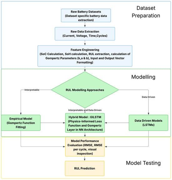
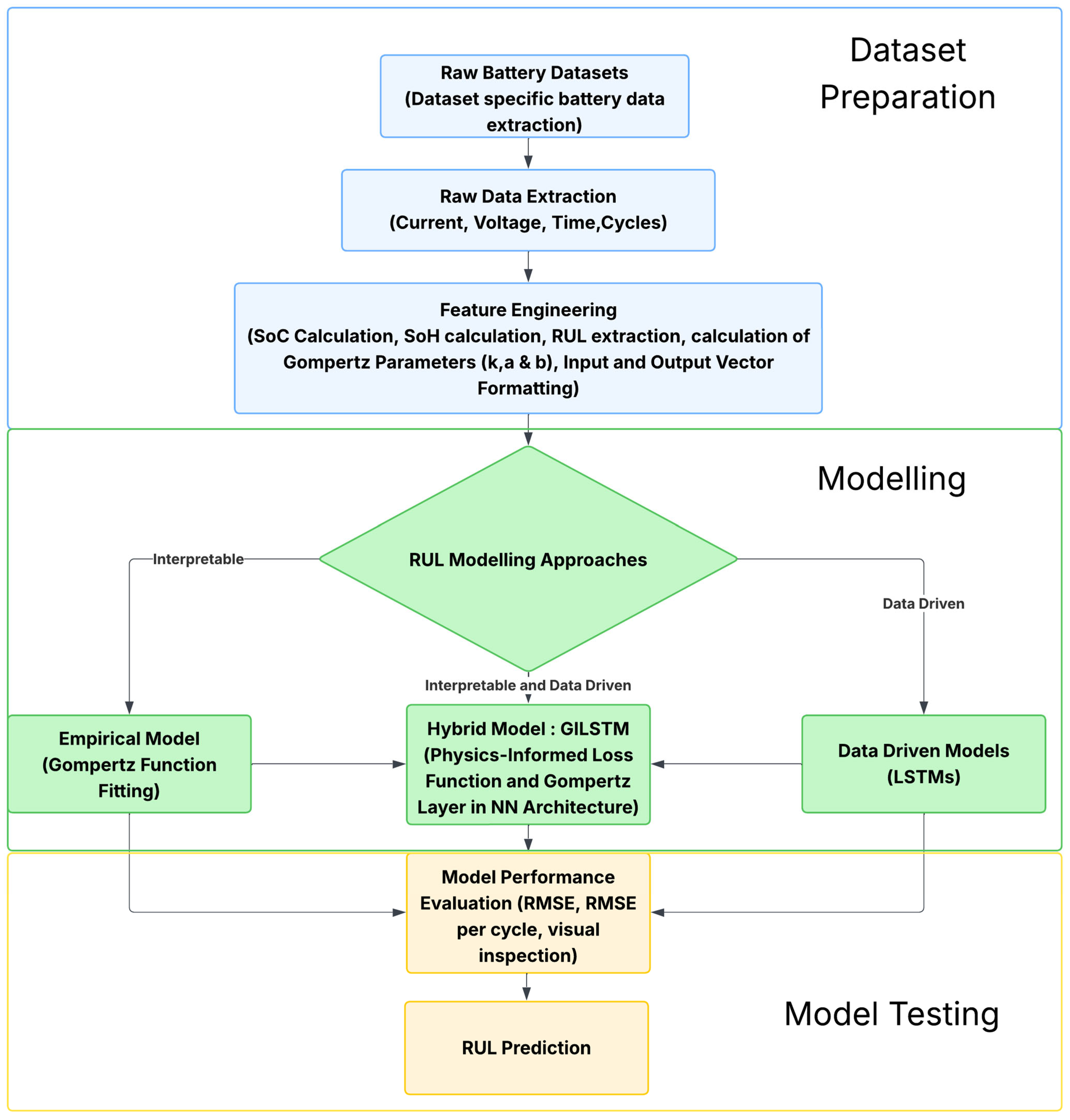
This section outlines the basis for using the Gompertz function, the dataset characteristics and the methodological framework employed in this study. It describes and explores the dataset used, the implementation of pure data-driven models utilizing LSTMs, empirical modeling based on the Gompertz decay function and a novel hybrid approach: Gompertz-Informed LSTM (GILSTM). This hybrid architecture proposes combining the generalizability of the data-driven techniques with the interpretability and robustness of an empirical modelling approach to accurately estimate Remaining Useful Life (RUL) at specific State of Health (SoH). The overall workflow adopted for this study is visualized in Figure 1 below.
Figure 1.
Data and machine learning pipeline.
The key parts of Figure 1 were dataset preparation, modelling and model testing. Dataset preparation involved acquisition of available online LFP battery datasets, conversion of the raw data to pandas data frames where variables such as current, voltage, time and cycles were extracted from the dataset and using Equation (1), these data was feature-engineered to calculate SoC thus, by obtaining the maximum SoC relative to nominal capacity, the SoH of each cell at each cycle was computed. The RUL was extracted for each cell at 70% normalized SoH and the resultant SoH curves were used to compute the Gompertz parameters (k, a, and b) to be used as physical constraints for hybrid models. Modelling involved comparing three distinct approaches to predict RUL. Model testing was the final stage used to evaluate each model’s effectiveness.
3.1. Basis for Using Gompertz Parameters for RUL Prediction
3.1.1. Monotonicity and RUL Prediction
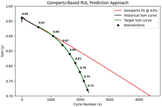
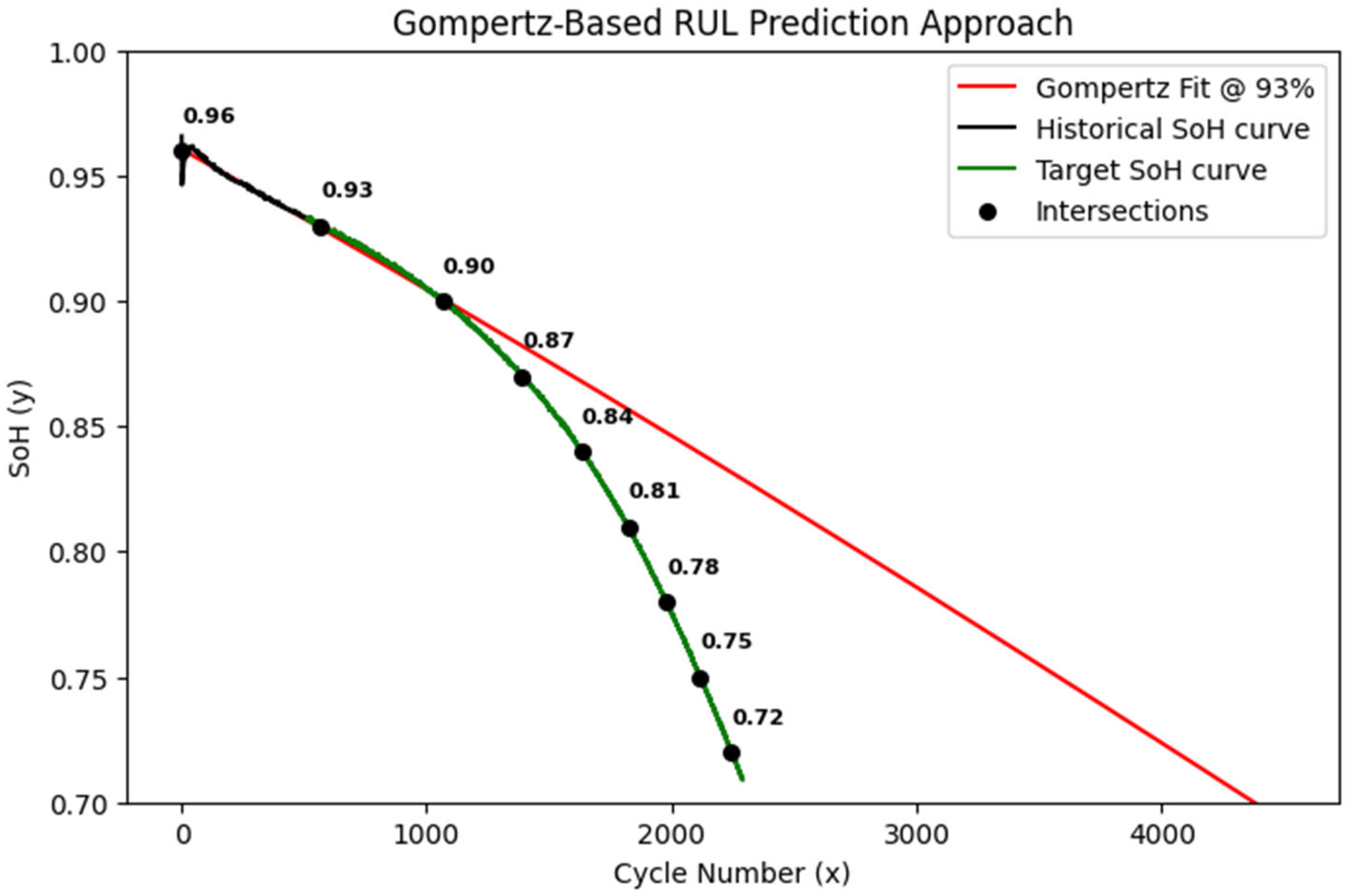
LiB capacity degradation is inherently a downward monotonic process. While predicting the SoH at future cycles is a common approach to estimating the RUL, direct multistep forecasting often suffers from error accumulation (drift) as the prediction horizon increases. To address this contention around predicting RUL, this study proposes an inverse mapping strategy. Rather than predicting the SoH for a given cycle, the model predicts the number of cycles required to reach 0.7 SoH threshold. Thus, RUL prediction is reformulated as determining the number of cycles the battery in its current state will take to reach its End of Life (EoL) threshold. This approach leverages the monotonic nature of capacity degradation, mapping observed data to a specific destination (the RUL at EoL). As illustrated in Figure 2, the proposed method predicts the point of failure by estimating the number of cycles required to reach a SoH of 0.7, enforcing a strict monotonic decay consistent with physical capacity degradation.
Figure 2.
Schematic of the proposed inverse mapping prediction.
Unlike traditional methods that forecast SoH from cycles or predict RUL, this paper’s approach uses an LSTM to predict the k, a and b (Gompertz parameters) and uses the inverse Gompertz equation to calculate the corresponding RUL from the x-axis. The Gompertz model can on its own be used to predict close SoH intervals, for example, in Figure 2 the Gompertz fit for SoH data from Beginning-of-Life (BoL) to 93% SoH (511 cycles of historical data) can be used to calculate the cycles needed to reach 0.9 SoH but can an LSTM trained using constraints informed by the Gompertz model accurately predict the k, a, and b parameters that would calculate the RUL accurately? The Gompertz fit at 93% SoH approximates a RUL of 4452 cycles. The theoretical Gompertz degradation path (red curve) serves as a physics-informed constraint, guiding the LSTM’s k, a, and b values to predict the SoH curve (green line) while ensuring monotonic degradation behavior. By predicting the RUL, the model combines the data-driven benefits of neural networks with physics informed constraints derived from the Gompertz growth model [41].
3.1.2. The Gompertz Model
The Gompertz model [41] is a widely established sigmoidal function commonly used to describe growth and degradation processes, owing to its asymptotic behavior, interpretability and ability to model nonlinear trends such as growth and degradation phenomena. In this study, the Gompertz function is used to approximate the capacity degradation curve of LFP batteries and estimate their RUL. The general form of the Gompertz function [41] is defined in Equation (3). The Gompertz function will be referred to as .
where
- denote the normalized capacity at cycle x fitted to the Gompertz function;
- is a scaling factor representing initial capacity;
- is a shape parameter controlling the shift of the curve;
- controls the rate of capacity degradation.
The model parameters (k, a, b) are estimated using non-linear least squares optimization. Equation (3) can be rearranged to Equation (4) to solve for x (cycles) given a specific target SoH (), facilitating the inverse mapping strategy described in Figure 2. The inverse Gompertz function will be referred to as .
Furthermore, to ensure the neural network adheres to physical degradation laws, the differential form of the Gompertz equation is utilized as a constraint during training. This enforces a Physics-Informed framework where the network outputs satisfy the rate of change defined by Equation (5). The first derivative of the Gompertz function will be referred to as while the second derivative will be referred to using .
By integrating Equation (5) into the loss function, the model is constrained to obey the mathematical properties of the Gompertz degradation trend, ensuring robust and interpretable RUL predictions.
3.2. Dataset Acquisition and Description
The dataset used for experimentation and pipeline development in this study was the Huazhong University of Science and Technology (HUST) battery dataset [42]. The HUST battery dataset was downloaded directly from Mendeley data. The raw HUST dataset comprises of charging and discharging data from 77 LFP cells, each with a nominal capacity of 1.1 Ah. From the data, all cells were cycled using a standardized charging protocol, with different multistage discharge protocols applied to the cells at a constant temperature of 30 °C to ensure thermal consistency across the dataset. The dataset is meant to be used to model battery health, thus relevant to the study in this paper. The raw HUST data has been packaged in pickle format (.pkl) and are serialized python objects that had been converted into a byte stream for storage purposes.
3.3. Dataset Analysis and Preparation
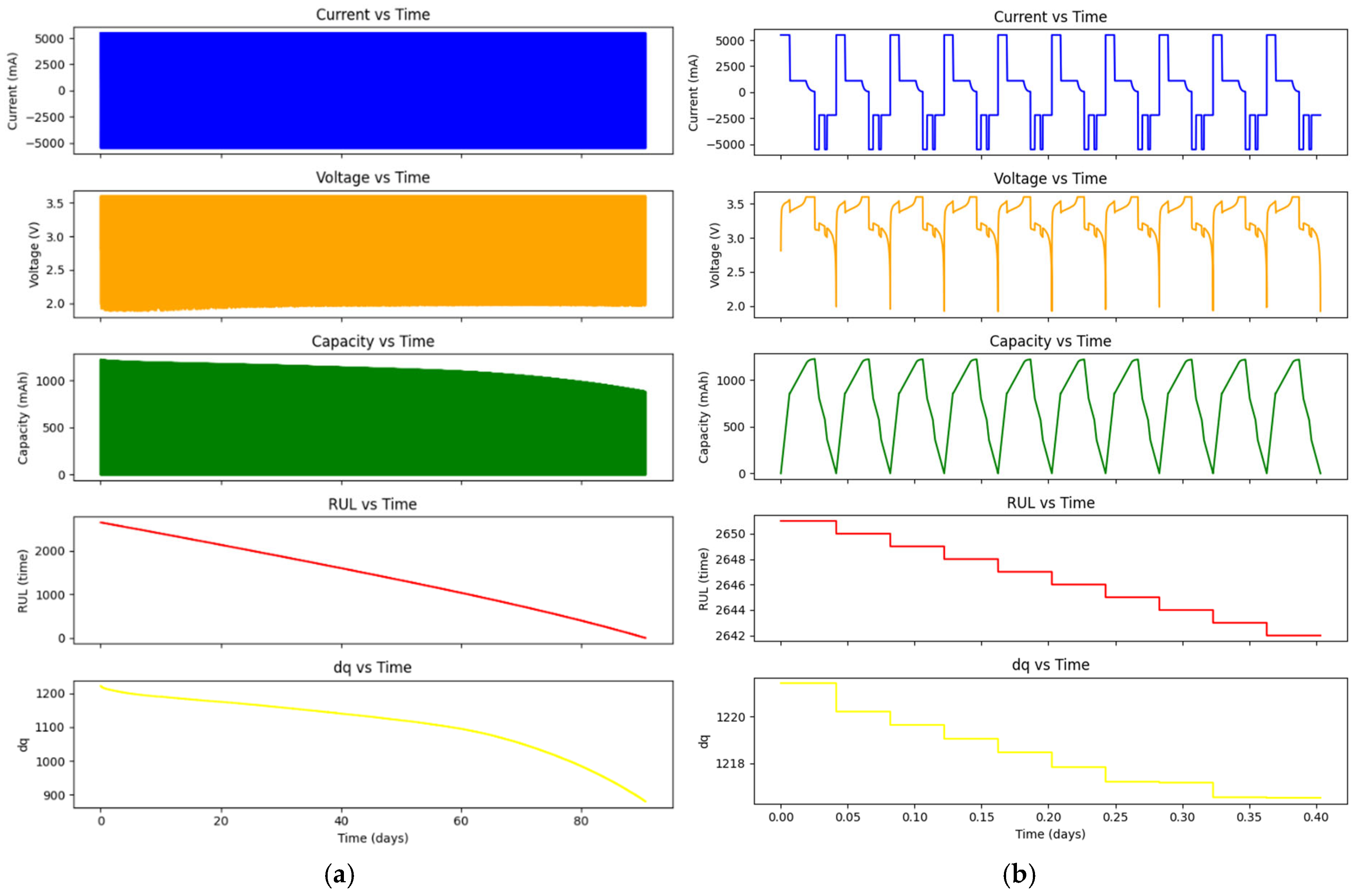
The raw HUST data were stored in dictionary format, that dictionary contained three nested dictionaries, the first contained data representing the calculated RUL at each battery cycle, the second contained the battery capacity after each cycle and the third contained data indicating the charging status, cycle number, current in milliamperes, voltage, capacity of stored power and the time since the cycle started. To conduct the study in this paper, the data was aggregated into a refined dataset. The refined dataset includes five dependent variables: current, voltage, cell capacity (Q), RUL, and change in capacity (dq), as well as two independent variables: time and cycle number. Figure 3 shows how these variables change over time for cell 2–2. The plots are of the dependent variables over time for all cycles of cell 2–2 from the HUST dataset on the left (a) and on the right (b) are the same plots over time but only for the first ten cycles.
Figure 3.
The plots of the dependent variables over time for cycles of cell 2–2.
The RUL of the cell equaled zero when the usable cell capacity dropped to 880 mAh (80% of the nominal capacity). Figure 3b zooms in to the first ten cycles (9.7 h) of Figure 3a, showing how the dependent variables evolved with each charge-discharge cycle within those 10 cycles, while Figure 3a shows how those dependent variables evolved over the entire lifespan of the battery (2651 cycles/90 days). The HUST dataset had data from variables of voltage, current, time, capacity, dq and cycles to model SoH and RUL, and it was required to understand the relationship between these variables and how they can be used to obtain SoC and SoH. For the SoC to be computed, the Coulomb Counting SoC estimation formula shown in Equation (1) was used because SoH is defined as the ratio of the capacity of a battery in a used state and a new state [43,44,45]; moreover, since the Coulomb Counting SoC equation uses the rated capacity instead of the current capacity, this detail is reinforced. As mentioned earlier the coulomb counting equation typically uses the nominal capacity to calculate SoC, if a SoH degradation model such as an LSTM or a Gompertz model is used, the capacity can be adjusted such that each percentage value of the SoC from 0% to 100% of each cycle is corrected, that is, 1% should represent 1% of the current capacity not rated capacity, for early, mid and later cycles. The SoH formula is represented as in Equation (6), where stands for the cell capacity at time and is the nominal capacity of the cell.
Since the HUST cells were charged and discharged to more than the nominal capacity of 1.1 Ah, each cell was normalized by 115% of 1.1 Ah to ensure they are bound between 0 and 1. This is attributed to the conservative manufacturer ratings and the capacity buffer typically found in new cells [46,47]. By using a normalization factor of 1.265 Ah (115% of nominal capacity), the SoH normalization in Equation (7) accounts for the fact that new high-quality cells often exhibit an initial capacity significantly higher than their labelled nominal capacity. This ensures that normalized SoHs do not exceed 1.0 at the Beginning of Life (BoL) which would otherwise distort the training of machine learning models like LSTM; thus 80% of the nominal capacity is normalized to 70% SoH.
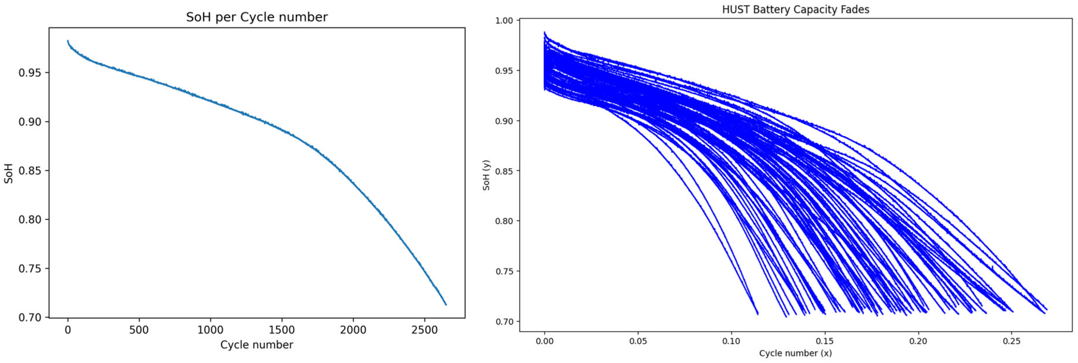
Following the completion of data preprocessing and calculations, the capacity values for each cycle were extracted, enabling subsequent analysis of degradation trends. For training, validation and testing purposes, the dataset was split with the ratio 72:14:14, resulting in 55 cells for training, 11 cells for validation and 11 cells for testing, the exact splits were based on BatteryML’s [40] train–test splits, this was to ensure consistency when comparing results. In Figure 4, the SoH values obtained from the SoH normalization formula Equation (6) are used and the cycle number has been normalized by 10,000 cycles, the expected upper limit number of cycles. The batteries in the HUST dataset used more than the nominal capacity of 1.1 Ah with many reaching 1.21 Ah. To ensure uniformity among all the datasets, 1.265 Ah was used as the normalizing constant for the dataset used as shown in Equation (7).
Figure 4.
The plot of normalized SoH versus cycle number for cell 2–2 (left) and a plot of SoH versus normalized cycle count is plotted for all 77 HUST cells (right).
3.4. Modeling
3.4.1. Gompertz Model Formulation
The Gompertz model is a growth model developed by Benjamin Gompertz in 1825 to model human mortality [41]. The Gompertz model was utilized in two experiments, the first set of experiments fit the model on entire SoH curves like those shown in Figure 4, thus extracting their final k, a and b, then finally calculating the RUL using Equation (4) where y = 0.7 and checking the Gompertz model’s ideal performance. This method is referred to as the baseline Gompertz fit. The second method was testing the Gompertz model’s real time RUL estimation performance from cycle 1 to cycle N where N ranged from value 2 to value 2689 (the longest cell lifespan of any of the HUST cells). For the second method, , Equation (4), was also used. This method is referred to as Real-Time Gompertz Testing. Data analysis was conducted to explore the relationship between the Gompertz parameters k, a, and b, and the battery RULs.
- Baseline Gompertz Fit
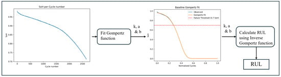
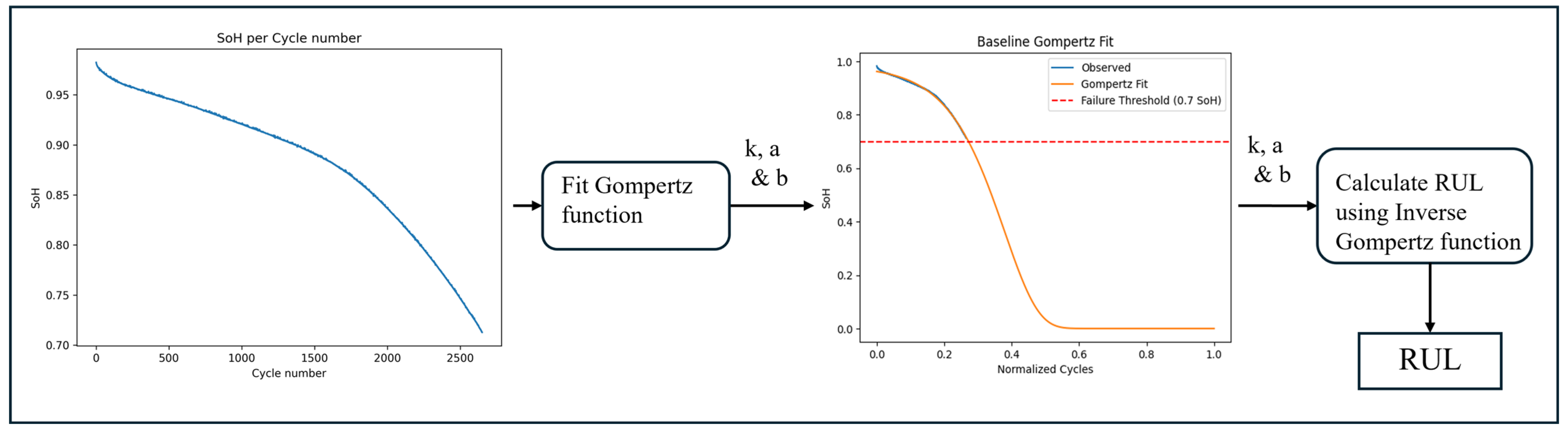
In an ideal situation, the entire SoH curve of each battery is known by some form of successful extrapolation thus fitting to these curves results in values of k, a and b whose calculated RULs should have very little deviation from the target RULs. By doing this, the study shows the potential performance of the Gompertz model. Figure 5 shows the pipeline used to calculate the RUL using .
Figure 5.
Schematic of the RUL estimation framework using and .
The observed SoH on the left was fitted to the model to extract parameters k, a, and b, these parameters are used as targets in the GILSTM later. The parameters were used to calculate the exact point of intersection with the failure threshold by using , Equation (4), where y = 0.7, resulting in predicted RUL values.
- B.
- Real-Time Gompertz Testing
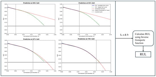
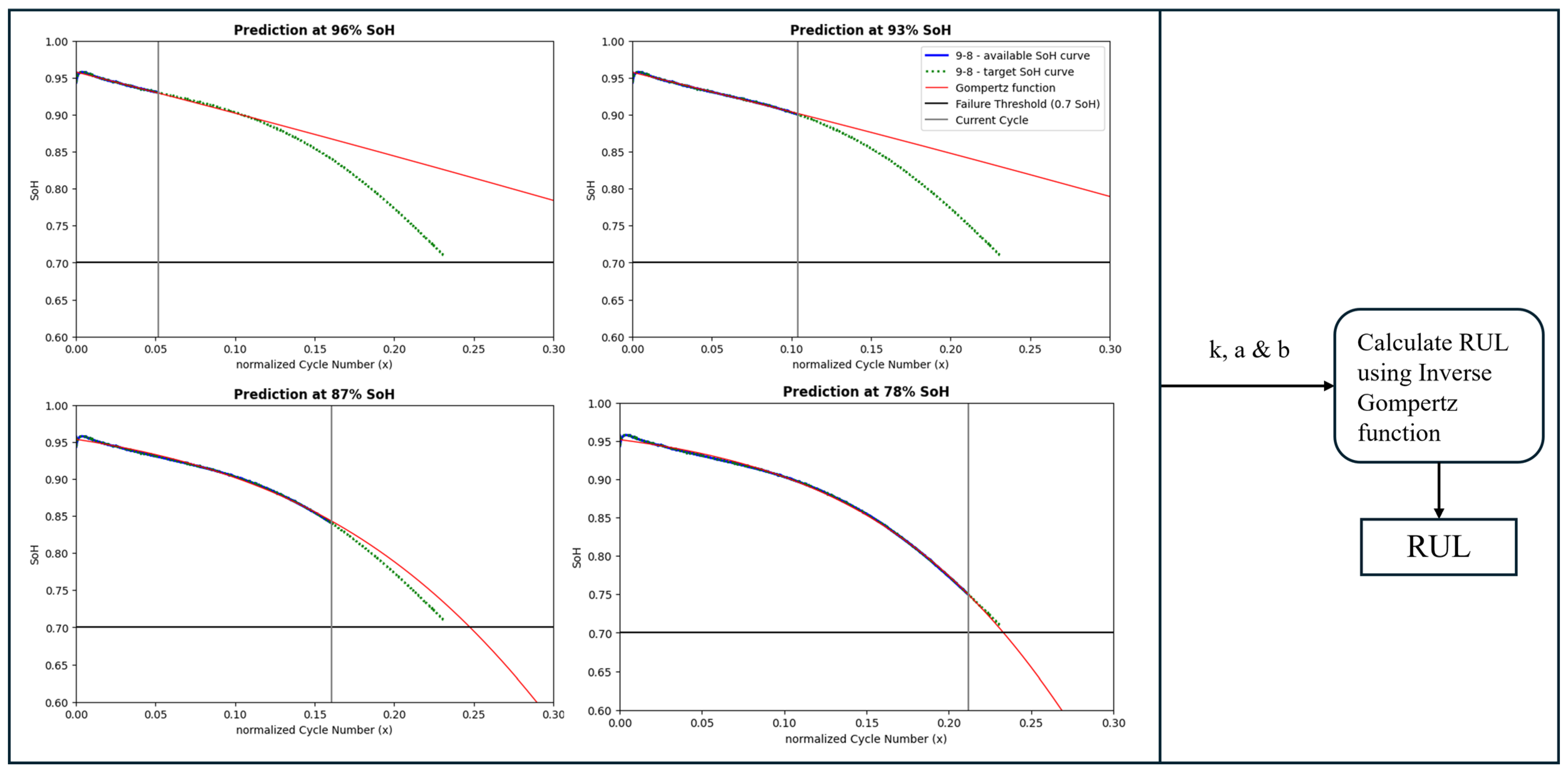
In practice, the complete SoH curves are not known if the cell has not reached its RUL, the curves need to be approximated from the known values of SoH. Each cell would have SoH values ranging from cycle 1 to cycle N where N ranged from value 2 to value 2689 (the longest cell lifespan of any of the HUST cells), with an interval of 1 cycle. The schematic pipeline for this is shown in Figure 6. As illustrated in Figure 6, the parameters k, a and b are subsequently used in Equation (4) to estimate the RUL by extrapolating the cycle x at which the SoH drops to 0.7 due to normalization in Equation (7) the SoH values of 110% to 80% are represented within the range 0.96 to 0.7.
Figure 6.
Schematic of the real-time fitting procedure.
Figure 6 above describes how the Gompertz model fits on available data and how RUL is calculated at different cycle numbers and SoH thresholds. The Gompertz model was fitted on truncated SoH curves representing different stages of battery life (96%, 93%, 87%, and 78% SoH). The vertical gray line indicates the current cycle available for fitting; the red curve shows the Gompertz model’s extrapolation used to calculate RUL at that specific cycle. The main limitation was how to capture long temporal dependencies, especially given how the SoH curve has a non-linear shape. When calculating the RUL, the values were multiplied by 10,000 to obtain the non-normalized RUL values.
3.4.2. Long Short-Term Memory (LSTM) Models
LSTM networks [48] are a type of recurrent neural network (RNN) capable of learning long-term dependencies in sequential data. Due to their memory nodes, LSTMs are particularly effective at modelling time series data with temporal correlations, such as battery capacity degradation patterns across multiple charge–discharge cycles. In this study, two LSTMs were developed to model SoH to RUL using two separate strategies and the same models were used as the backbone neural networks in the GILSTM Section 3.4.3. The two models can be classified in this manner:
- An LSTM that directly predicted RUL from SoH values (LSTM1);
- An LSTM that predicted the next cycle’s SoH from historical SoH values (LSTM2).
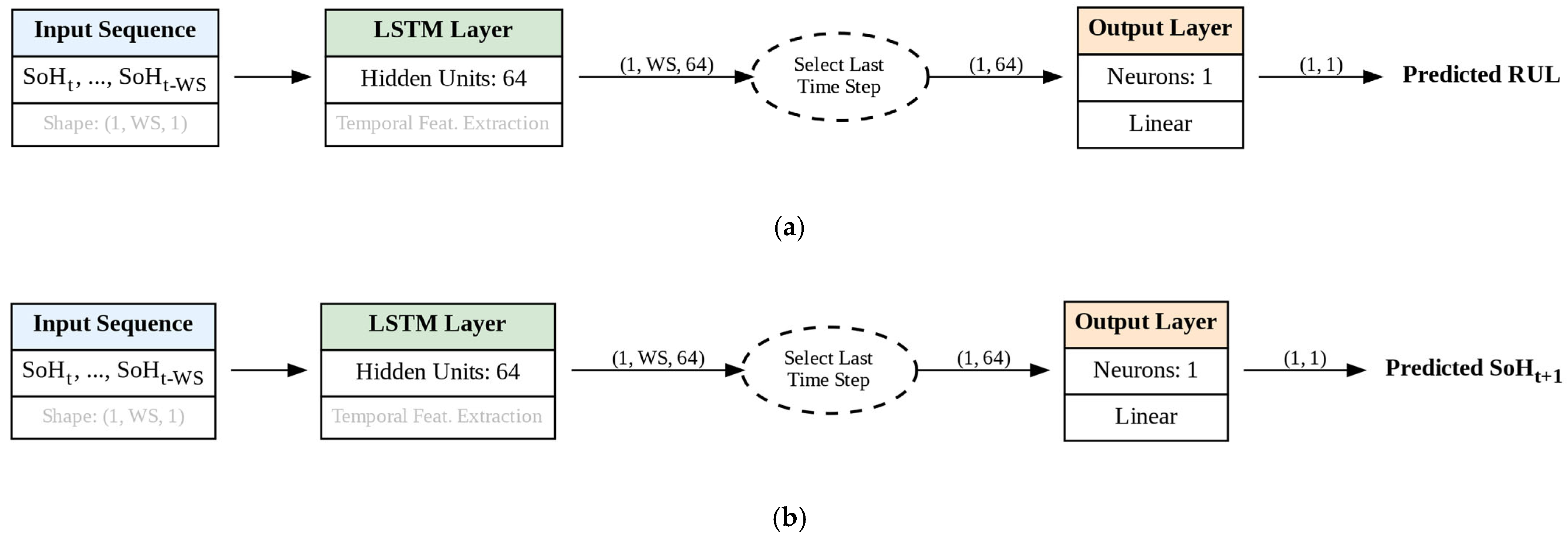
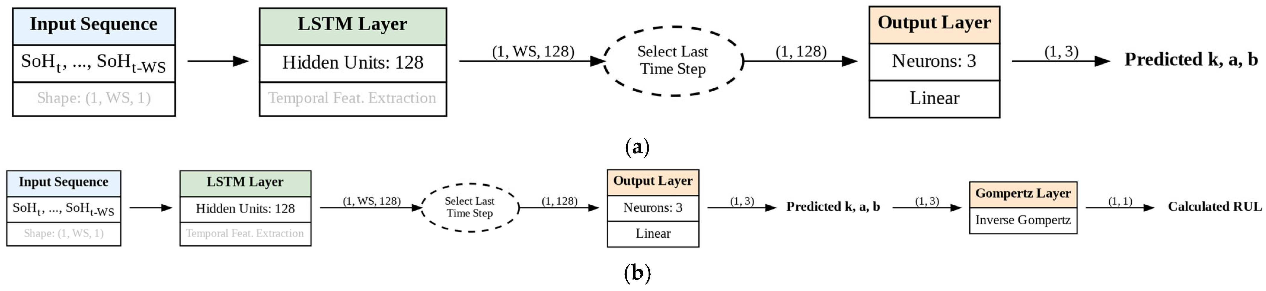
These models were used as baseline Blackbox models. For each of these models, the same backbone LSTM predictor was used with the main differences being the mentioned outputs, the training strategy as well as testing strategies. The architecture of each of these models is shown in Figure 7. Both models take a sequence of normalized SoH values as input, these values are derived from the SoC calculations over a fixed window of prior cycles, here a window size of 100 cycles is used. LSTM1 outputs a single RUL prediction. LSTM2 outputs the next cycle’s SoH value, the RUL is obtained from it by recursively popping out the first value in the window, shifting the remaining window forward by one and popping in the predicted SoH value at the end of the window then running the model on this new window. The number of cycles needed to output a SoH prediction lower than 80% of the nominal capacity is taken as the predicted RUL. This type of LSTM is known as a sequence-to-one LSTM.
Figure 7.
(a) The labeled architecture for the SoH-to-RUL LSTM (LSTM1). (b) The labeled architecture for the SoH-to-SoH LSTM (LSTM2).
These two models are baseline data-driven LSTM models for comparison with the GILSTMs. The approaches leverage the LSTM’s ability to capture non-linear and temporal dynamics in battery behavior enabling accurate RUL estimation. Since these two models were formulated as similar sequence-to-one regression tasks as seen in Figure 7, their input tensors are similar and of the shape [batch_size, window_size, 1], where the window_size (WS) refers to the number of time steps used in each prediction. Experiments reported in this study were conducted with a window size of 100.
Training Setup
Model training and inference were conducted on a POSIX-compliant Linux x86_64 system with a P100 GPU and on a POSIX-compliant, heterogeneous linux system primarily based on the ARM architecture with 4 NVIDIA GH200 GPUs. The LSTM networks were trained using the Adam optimizer [49] with an initial learning rate of 1 × 10³. To improve convergence, a StepLR learning rate scheduler was employed with a step size of 200 epochs. The Mean Squared Error (MSE) was used as the loss function, and performance was evaluated using Root Mean Squared Error (RMSE) on both training and validation datasets. The models with the best validation loss were saved. The number of training epochs set at 1000 as shown in Table 3 was determined empirically by monitoring the validation RMSE. Training continued for all 1000 epochs but only the best model was saved.
Table 3.
LSTM Key Training hyperparameters.
3.4.3. Gompertz-Informed Long Short-Term Memory (GILSTM) Models
In this study there were three GILSTM models developed to leverage the advantages of LSTMs and to model battery capacity degradation. The three models were classified as follows:
- A GILSTM that directly predicted the parameters k, a and b from SoH values (GILSTM1) trained only on SoH data from the first 100 cycles only. For the inference stages, the predicted k, a and b were passed through an inverse Gompertz layer to predict each test cell’s RUL.
- A GILSTM that directly predicted the parameters k, a and b from SoH values (GILSTM2) trained on SoH data from all cycles. For the inference stage, the predicted k, a, and b were passed through the inverse Gompertz layer to predict each test cell’s RUL. This inverse Gompertz layer is based on the Equation (4).
- A GILSTM that predicts RUL using LSTM2, the model predicts the next cycle’s SoH from historical SoH values (GILSTM3), when used recursively, it can predict the RUL. was fitted on the recursively output SoH curve and using the generated k, a, and b parameters were passed through the inverse Gompertz layer to predict each test cell’s RUL.
GILSTM1 and GILSTM2 both utilize the architecture described in Figure 8. The architectures are different depending on whether the model was training, Figure 8a or inferencing, Figure 8b. When inferencing, the was used to calculate RUL within the inverse Gompertz layer.
Figure 8.
(a) The architecture for GILSTM1 and GILSTM2 used in training. (b) The architecture for GILSTM1 and GILSTM2 used during inference.
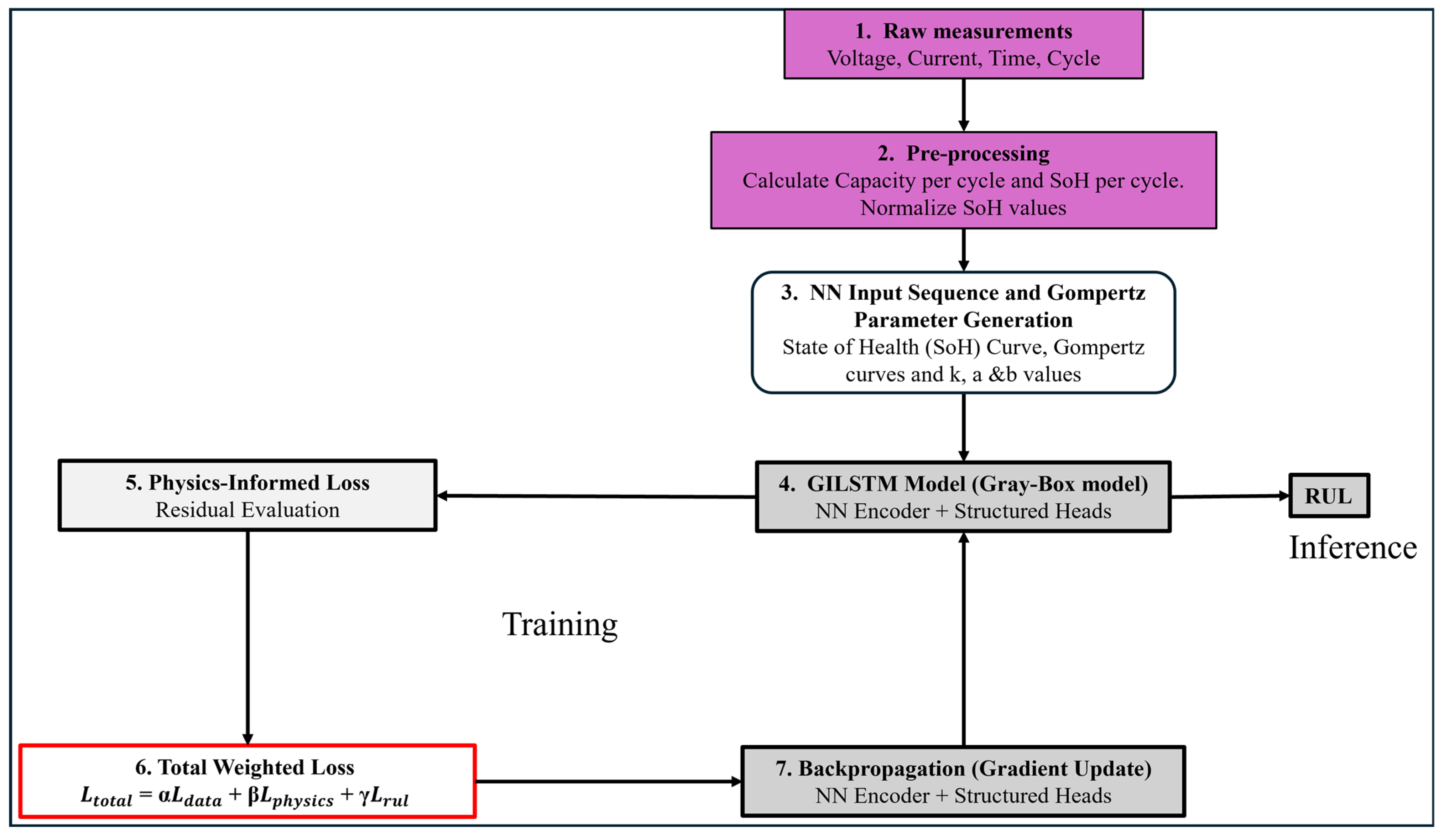
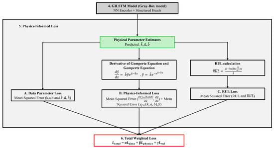
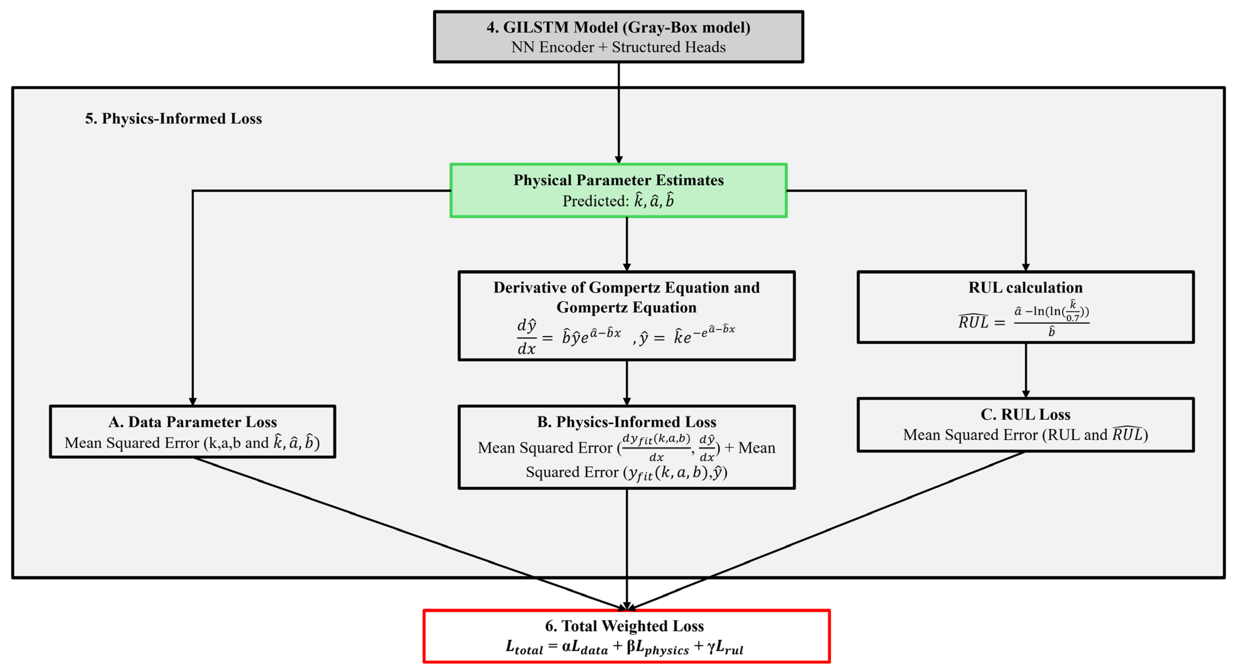
The GILSTM1 and GILSTM2 models were used to predict the parameters first to ensure that the models learnt the physical degradation of the battery’s capacities. Training of these models utilized the same hardware used to train and test the purely data-driven models. The training process of these Gray box models is shown in Figure 9 and utilizes a weighted loss comprising of data loss, physics loss and RUL loss to guide the training process. The Physics-Informed Loss function is described in more detail in Figure 10 and in Equation (9). The overall weighted function used in training combines the data loss, the MSE between the target k, a, and b and the predicted k, a and b, the physics loss, MSE between the target and predicted represented as and the MSE between the target and predicted represented as y and an RUL loss where the predicted k, a and b were passed through the inverse Gompertz layer with y set to 0.7, calculating the predicted RUL and then calculating the MSE between predicted RUL and target RUL. The GILSTM3 model leveraged the superior learning of the LSTM2 network to capture the underlying capacity fading shape and the used the capacity fade curve output from the LSTM2 to fit the parameters k, a and b of . RUL prediction from these fitted k, a, and b is then conducted. All models were developed and tested using the same hardware infrastructure as the purely data-driven baselines to ensure comparative consistency, moreover, Table 4 presents the training hyperparameters used in the GILSTM1 and GILSTM2 models. A curriculum learning [50] schedule was utilized to manage the multi-objective optimization of parameters (k, a, b), ordinary differentials and the final RUL.
Figure 9.
The training process for GILSTM1 and GILSTM2.
Figure 10.
The Physics-Informed Loss used for training GILSTM1 and GILSTM2.
Table 4.
GILSTM Key Training hyperparameters.
The orders of magnitude for α, β, γ were selected to normalize the gradient contributions, accounting for the differences in scale between the RUL values and the Gompertz parameters.
Summary of similarities and differences in GILSTM models’ architecture and methodologies.
Table 5 summarizes the shared foundations and distinct operational differences of the three Gompertz-Informed LSTM (GILSTM) models developed in this study.
Table 5.
Summary of similarities and differences in GILSTM Models.
The core similarities of the three GILSTM models are as follows:
- All three models combine the data-driven temporal learning of LSTMs with the physical interpretability of .
- Each of the three models produces the Gompertz parameters k, a, and b and eventually relys on the inverse Gompertz equation (Equation (4)) to determine the battery’s RUL.
- The models utilize LSTMs to capture non-linear degradation dynamics and long-term dependencies within the battery capacity data.
- All models take 100 SoH values as their inputs.
The core differences of the three GILSTM models are:
- Generation of Gompertz Parameters versus SoH curve forecasting: GILSTM1 and GILSTM2 generate Gompertz parameters k, a and b while GILSTM3 forecasts the SoH degradation curve then uses the Gompertz model to fit this predicted curve to extract the three Gompertz parameters k, a and b.
- Training objectives: GILSTM1 is specifically benchmarked on its ability to learn degradation from limited early life data (the first 100 cycles) whereas GILSTM2 is trained and tested on the entire lifespan of each training cell.
- Role of the Inverse Gompertz Layer: For GILSTM1 and GILSTM2, the inverse Gompertz layer is an integral part of the inference architecture used to convert parameters directly into RUL, for GILSTM3, the Gompertz parameters were used as a verification step for LSTM2’s recursive SoH predictions.
3.5. Evaluation Metrics
Five evaluation methods were utilized to evaluate quantitatively the performance of the proposed models: mean squared error (MSE), physics-informed loss function, root mean squared error (RMSE), RMSE per Cycle and RMSE at cycle 100.
- Mean Squared Error (MSE): measures the average of the squares of the error [43] as illustrated in Equation (8).
The MSE is sensitive to outliers and used in regression models. Used when training all models, when training GILSTM1 and GILSTM2 the MSE was used to formulate the physics-informed loss function as shown in Figure 10.
- b.
- Physics-Informed Loss Function
The primary aim of the GILSTM1 and GILSTM2 architectures was to ensure that the models explicitly penalize the model for disobeying downward monotonicity. captures the trend of downward monotonicity from the SoH curves, to achieve that the MSE utilizes (), , the RUL as well as the Gompertz parameters k, a, and b as shown in Figure 9, Equation (9) and in the weighted loss function shown in Figure 10. Use of was influenced by the PINNs paper [51] as well as the fact that had a very high correlation with the cell’s RUL. This resulted in a weighted loss comprising of data loss, physics loss and RUL loss to guide the training process.
where
- Data Loss (Ldata): The MSE between the target and the predicted parameters k, a and b;
- Physics Loss (Lphysics): The combined MSE of the predicted represented as y and its actual and its predicted and its actual ;
- RUL Loss (Lrul): The MSE between the target RUL and the value calculated by passing the predicted parameters through the inverse Gompertz layer;
- c.
- Root Mean Squared Error (RMSE): Square root of MSE as illustrated in Equation (10). Sensitive to outliers and is in the same unit as the original data. %RMSE is the RMSE divided by the mean target RUL.
- d.
- RMSE vs. Cycle
This is used to evaluate how the models RUL RMSE changes as batteries degrade across their cycle life, and confirms model generalizability over time.
- e.
- RMSE at cycle 100
This is used as a benchmark result particularly because of work from Severson et al. [31] and BatteryML [40]. Since predicting the RUL is harder in early stages, this benchmark is a realistic way of comparing the performance of different models on RUL prediction. This benchmark relies on testing the model on data from the first 100 cycles only.
4. Results
This section outlines the results from Gompertz data analysis, visualized and numerical results from the modelling processes, particularly the results of empirical modelling based on , pure data-driven models utilizing LSTMs (LSTM1 and LSTM2) and novel hybrid approaches: Gompertz-Informed LSTM (GILSTM1, GILSTM2 and GILSTM3).
4.1. Gompertz Data Analysis and Modeling Results
The initial experimentation with was to provide baseline and real-time results when using the Gompertz model for RUL prediction.
4.1.1. Gompertz Parameter Data Analysis and Baseline Gompertz Fit
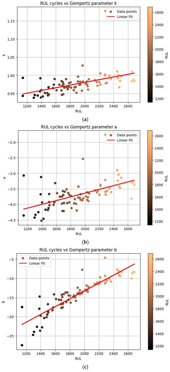
This section sought to establish justifiable reasons as to why the Gompertz model is suitable for helping LSTMs and other neural networks be more interpretable when predicting RUL. The results of these experiments are on full SoH curves. Prior to the development of RUL prediction models, the relationships between SoH and the Gompertz parameters as well as between RUL and the Gompertz parameters were investigated. This initial experimentation was to check whether the Gompertz model had captured any valuable information that was relevant to the cells’ RUL. The variables represented the values captured from the cell’s full SoH curves. It was found that the values for the Gompertz parameters k, a, and b shown in Figure 11, ranged between 0.93 and 1.2 for k, −4.6 to −1.5 for a and −28 to −4 for b. Parameter b shows a strong positive correlation with RUL. This reinforces the thought that and its parameters may be useful when predicting battery RUL.
Figure 11.
(a–c) The linear relationship between the Gompertz parameters k, a and b, respectively, with the RUL.
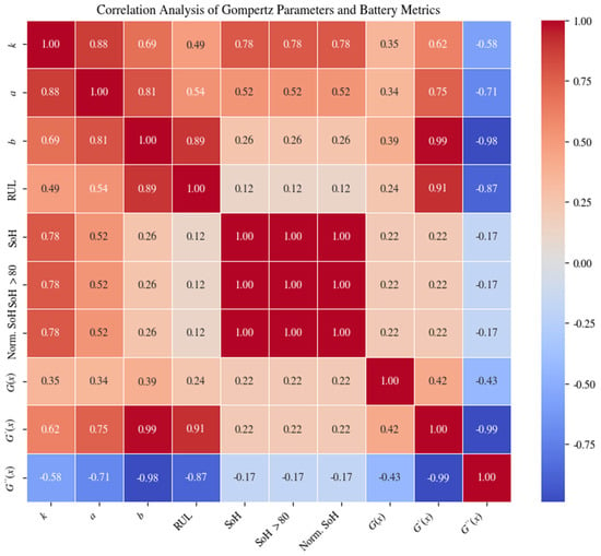
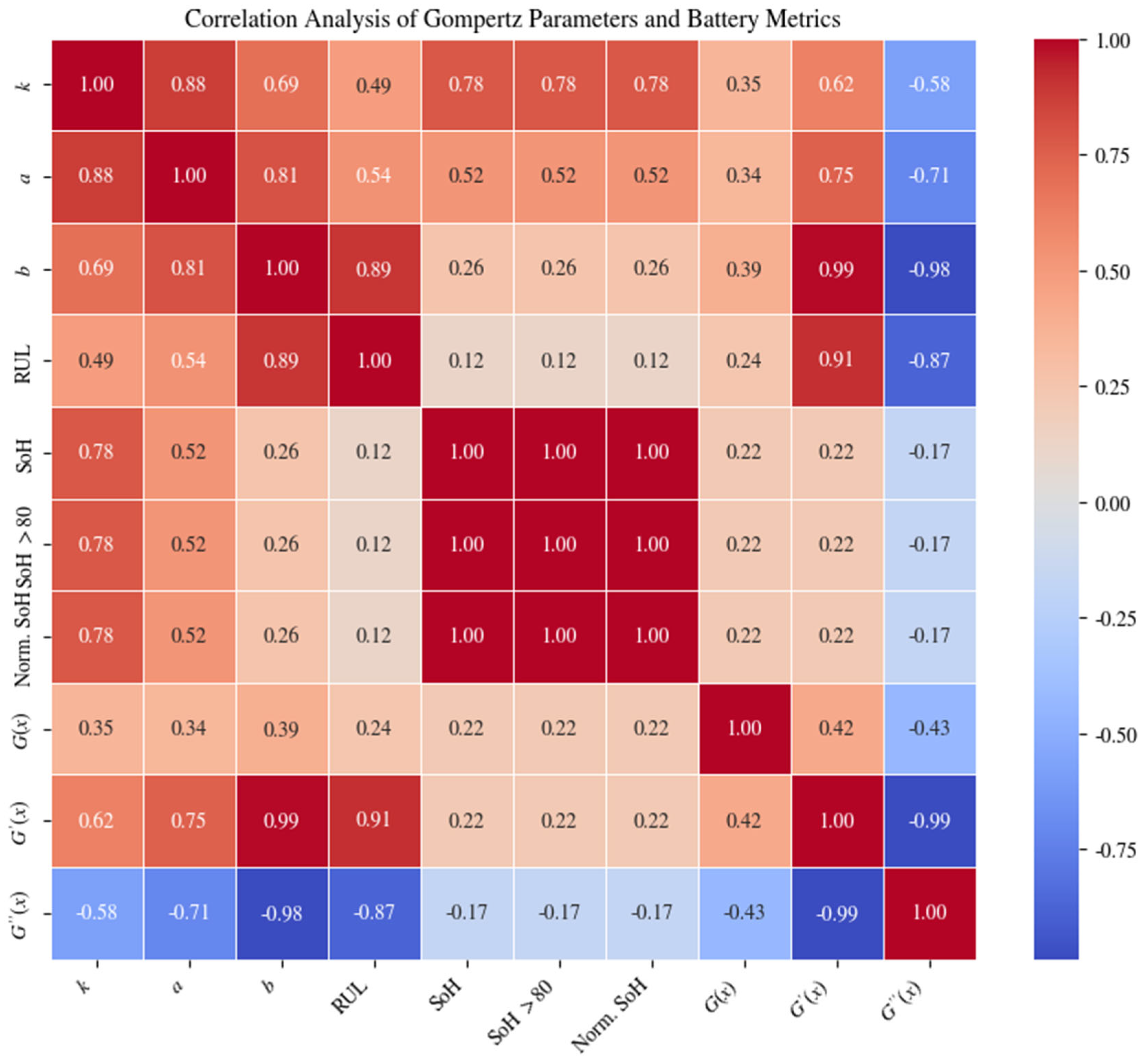
Moreover, Figure 11 confirms correlations for parameters k, a, and b with RUL seen in the correlation matrix shown in Figure 12 where parameter b has the highest correlation of 0.89 followed by parameters a and k respectively.
Figure 12.
The correlations between HUST data and Gompertz parameters.
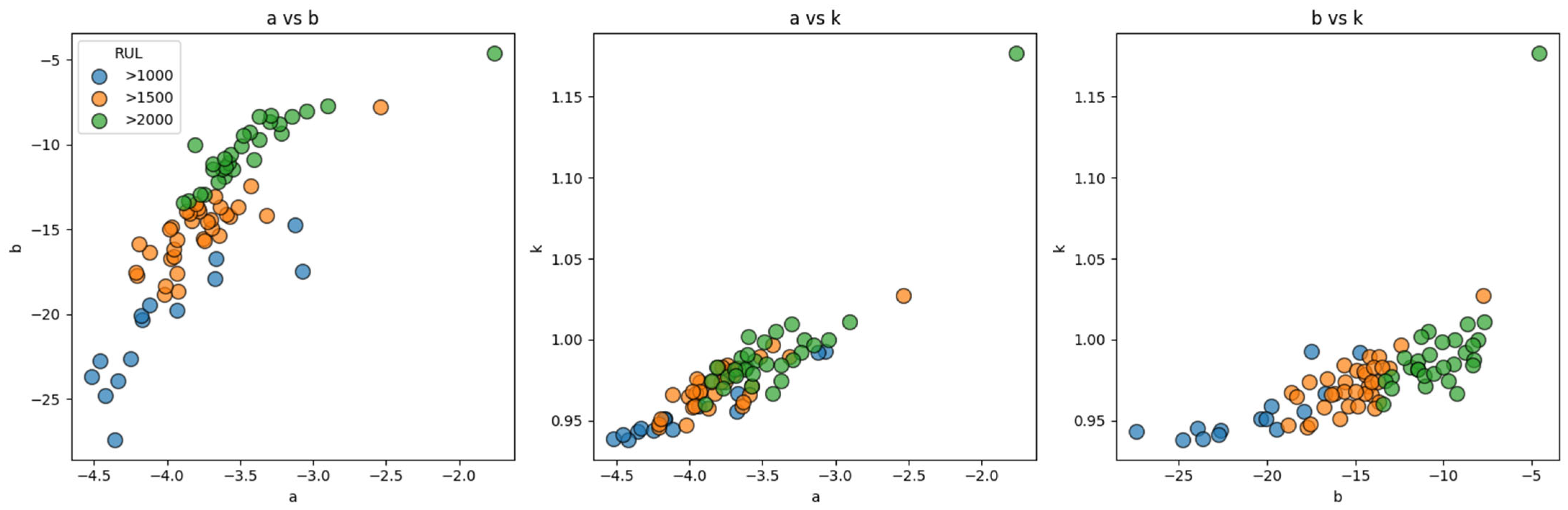
In Figure 12, what is particularly important is the high correlation between parameter b, and RUL. This high correlation informed the use of in the physics-informed loss function. The various tranches of RUL were 14 cells that had a RUL of 1000–1500, 34 cells with a RUL of 1500–2000 and 29 cells with a RUL of more than 2000. As part of the study, the relationship between these three various tranches of RUL and the Gompertz parameters k, a, and b was investigated and shown in Figure 13. The variable b delineates these three tranches precisely.
Figure 13.
The relationship between a and b (left), a and k (middle), and b and k (right) color-coded according to those RUL categories.
Figure 13 proves that can be used to confirm the RUL of a cell given complete SoH curves. Furthermore, the cells’ complete SoH curves were fitted on , and the RUL was calculated using (Equation (4)) resulting in a mean RMSE of 27.9 cycles (1.4%). Such results would be excellent, but they can only be calculated given the actual SoH curves are known beforehand.
4.1.2. Modeling Results
Below is Table 6, it represents the results of the various models developed in this study, as well as the results of comparable studies. The units of RMSE are in cycles.
Table 6.
Modeling results.
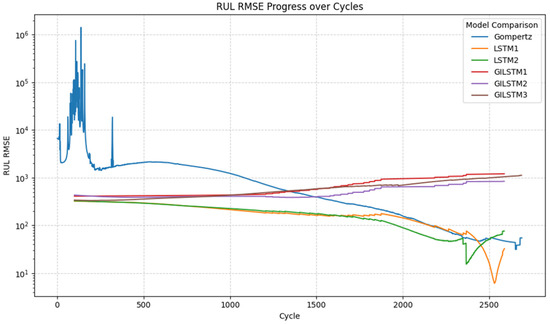
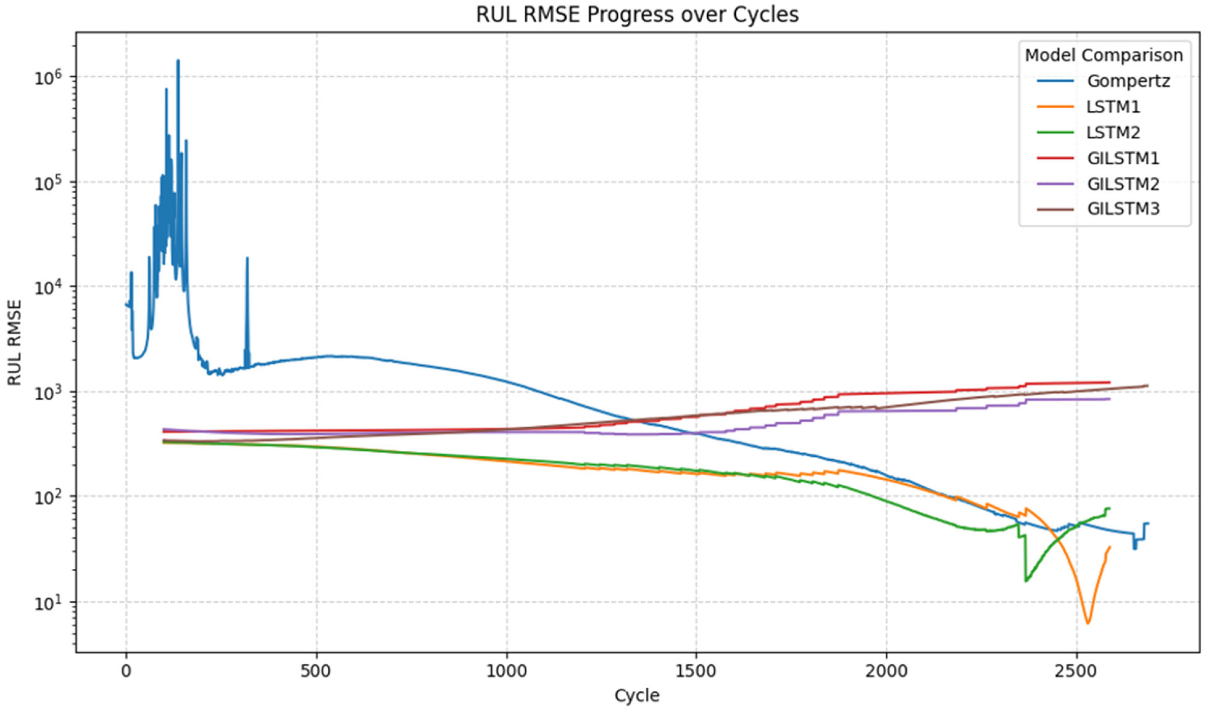
In Table 6, there is presented the performance of the developed models compared to the various baseline models. The baseline “Discharge” model used linear regression on capacity-voltage curves [51] whereas the BatLiNet model uses an Encoder–Decoder neural network with embedding spaces to achieve superior performance. The models developed in this study were also tested on RMSE per cycle resulting in Figure 14.
Figure 14.
The RMSE per cycle for each of the models developed in this study.
The relationship between SoH, and was also investigated for all cells and is shown in Figure A1. The performance failures of in the early cycles (before cycle 500) can be attributed to the high variability of the Gompertz parameters and large derivative values exhibited by the Gompertz as shown in Figure A1. As seen in Table 6 and Figure 14, LSTM1 and LSTM2 had the best performance at all stages of life.
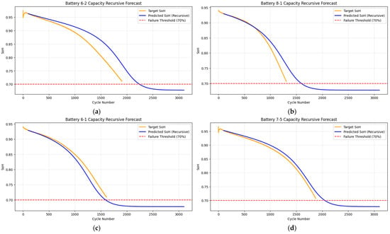
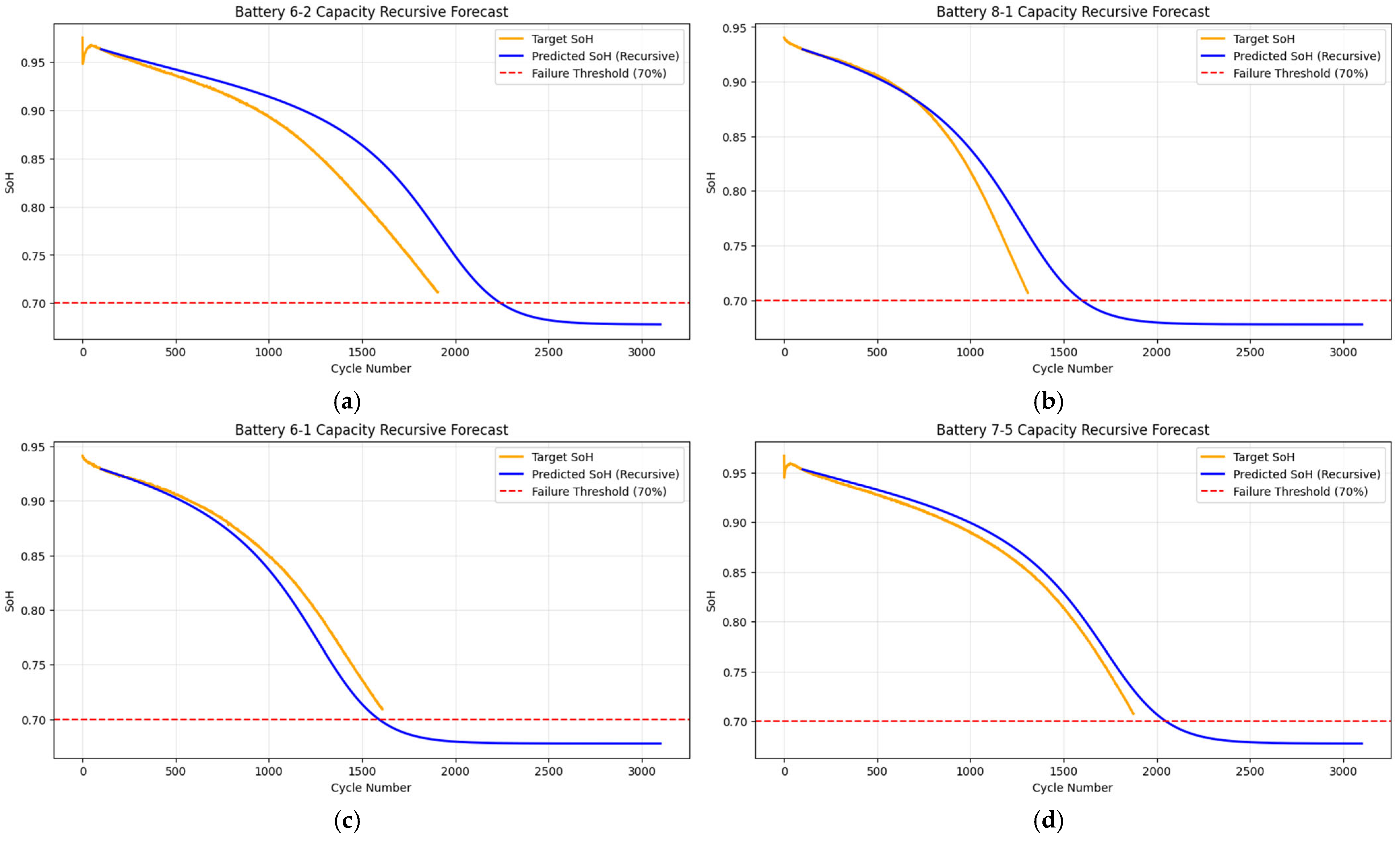
The various capacity forecasts were visually inspected to ensure they resulted in what was expected. Figure 15 below represents some of the test cells with their target SoH and their predicted SoH, these are the curves predicted by LSTM2 since the other models predict direct RUL values instead.
Figure 15.
The target and predicted SoH curves from LSTM2 for cells 6-2 (a), 8-1 (b), 6-1 (c), and 7-5 (d).
4.1.3. Operationalization of Gompertz Parameters
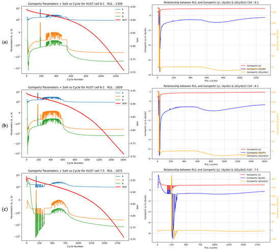
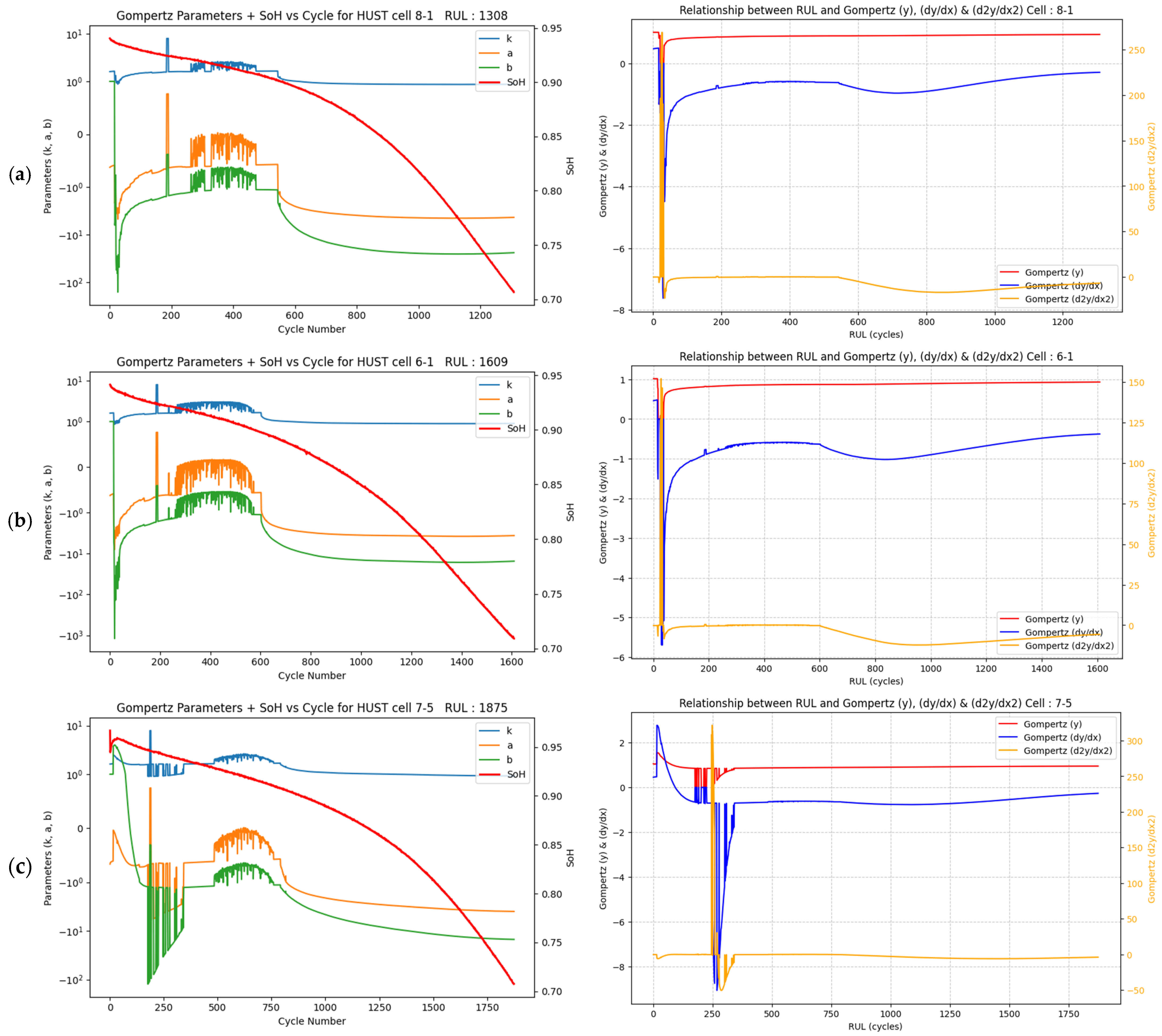
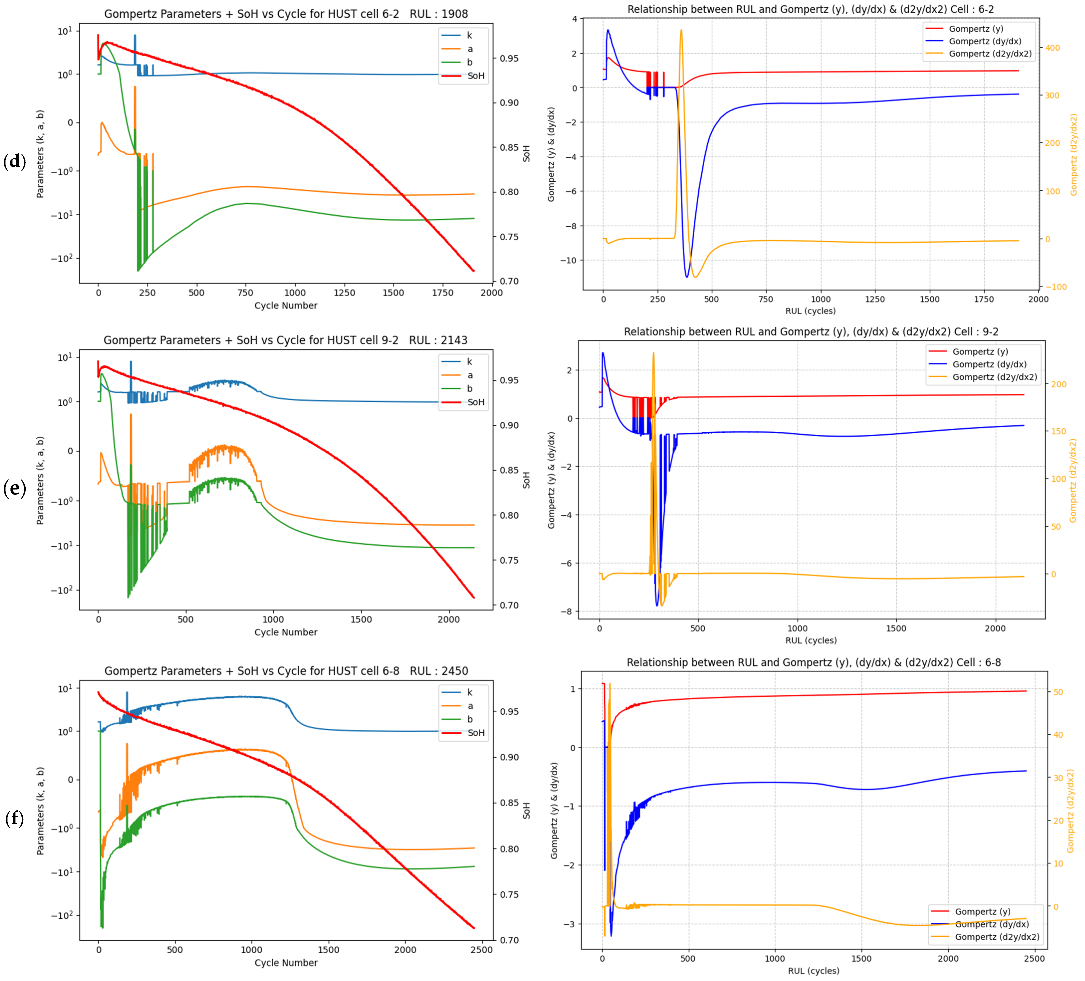
The Gompertz parameters k, a, and b, and offer significant operational utility for BESS management. A critical observation from the longitudinal analysis of the HUST dataset was the transition from high parameter variability in early life to low and stable variability as the SoH approached the point of maximum curvature in the degradation curve and into later life stages. Figure 16 presents 6 sample cells and the values of respective Gompertz parameters (k, a and b), and .
Figure 16.
The Gompertz parameters, and SoH curves for cells 8-1 (a), 6-1 (b), 7-5 (c), 6-2 (d), 9-2 (e) and 6-8 (f) for longitudinal analysis.
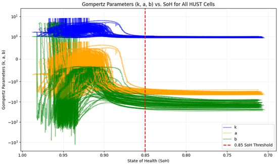
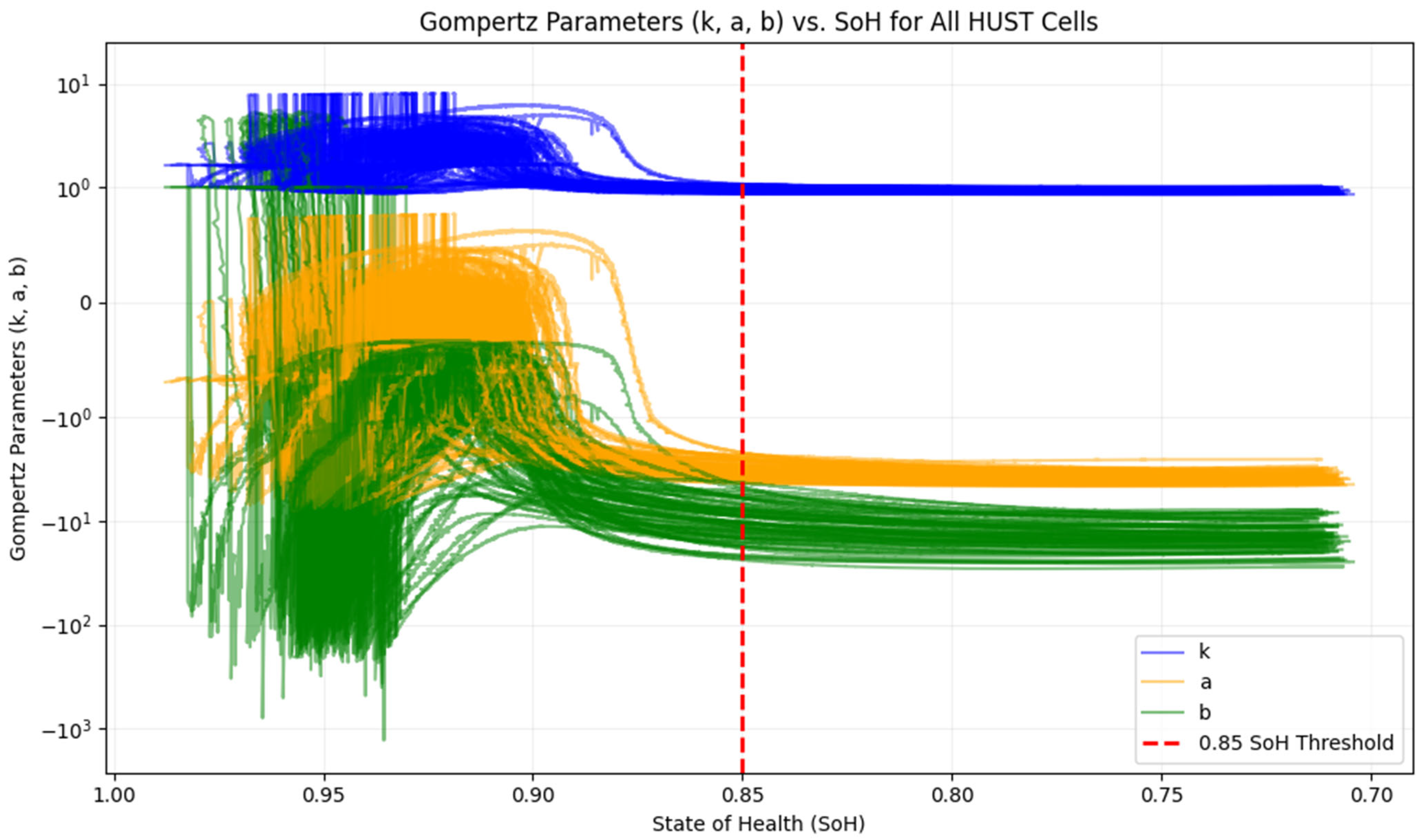
Based on Figure 16 a BESS operator can use the stabilization from high variability values as a trigger to transition from low-confidence RUL predictions to high-confidence RUL predictions. Before these points of transition, RUL estimates could be treated as provisional; after stabilization, the model’s RUL outputs would be of higher reliability. Moreover, based on such transitions a BESS operator can implement dynamic derating limiting the C-rates to mitigate the aging effects and the possibilities of BESS failures. Furthermore, a similar visualization of the Gompertz parameters of all the HUST cells illustrated in Figure 17, shows that all the cells’ Gompertz parameters evolve and stabilize by the 85% SoH point.
Figure 17.
The Evolution of Gompertz parameters with SoH for all HUST cells.
The stabilization of Gompertz parameters on Figure 17 and Figure A1 allows for a BESS operator to pre-emptively isolate or replace specific batteries that are nearing their accelerated aging phase to prevent failures in the overall larger pack. Moreover, batteries that exhibit parameters that fail to stabilize or diverge from the known k, a, and b can be flagged for unusual degradation which black-box RUL prediction models might overlook.
4.1.4. Ablation Study of GILSTMs
An ablation study was conducted as reported in Table 7 to identify the reason of failure of the GILSTM. This required four training experiments to isolate the source of failure which could have been the GILSTM’s architecture, the physics-informed loss function’s weighting or the instability in weighting optimization. The training and validation metrics for each of these configurations is present in Appendix B.
Table 7.
Ablation study of loss components of GILSTM performance.
The ablation study reported in Table 7 identifies that the underperformance of the GILSTM is not a result of optimization failure but a shortfall in the design of the architecture of the GILSTM. The results show that configuration A where only data loss was considered and configuration C, where complete physics loss was considered, achieved near identical test results indicating that the inclusion of the physics loss provided no additional predictive power. Configuration B shows that by not incorporating the RUL loss when training, the resultant model’s performance got worse. The significant degradation in performance when training only on stable data in configuration D did not result in better performance. The GILSTM’s failure likely stems from architectural choice and may be fixed by experimentation using more feature inputs such as k, a, b and their derivatives rather than just the SoH.
5. Discussion
The evaluation of the Gompertz model, LSTM models and GILSTM models in Table 6 and Figure 14 provide meaningful insights into their individual strengths, weaknesses and applicability for RUL prediction of LFP batteries. The Gompertz model offered advantages in physical interpretability with its parameters found to be strongly correlated to RUL, making it a suitable choice for real-world applications where interpretability is crucial. The Gompertz model was found to have poor standalone RUL performance before cycle 1000 where RUL prediction is very valuable, with some RMSE values hitting a million but had very good results after cycle 1000. These poor early-cycle stage results are attributed to the high variability behaviours seen in Figure 16 and Figure 17, as well as Figure A1 when the SoH is higher than 85–90%. Nevertheless, the Gompertz parameters, the and show significant evidence that they can be used to define a transitionary stage from where predicted RUL from the and the LSTMs can be regarded with higher confidence. Below 85–90% SoH and were seen to stabilize into smoother curves explaining the superior performance in mid-cycle and late-cycle stages; the performance in these stages catches up to LSTM1 and LSTM2, the best models in this study.
The extreme RMSE (861%) observed for the Real-Time Gompertz model at cycle 100 highlights fundamental mathematical instability of in high SoH regions (above 0.9). In these high SoH regions, calculation for RUL becomes numerically ill-conditioned. As y approaches the asymptote k, the double logarithm term ln(ln(k/y)) approaches −∞, causing even negligible noise to result in large RUL fluctuations. This is also seen in Figure 16 and Figure 17 as well as Figure A1. For the hybrid GILSTM variants, this instability manifested as gradient noise during training. When the optimizer encountered the extreme gradients produced by the inverse layer, the LSTM adopted a defensive learning strategy while the physics-informed model attempts to satisfy an underdetermined physical form where parameters a, and b are not yet constrained by the lack of observed curvature. Consequently, the GILSTMs failed to generalize to individual cell trajectories and instead centroided toward the mean k, a, and b parameter values of the training set. This suggests that Gompertz-based hybrid methods should be weighted lower during the early-cycle stage and higher during middle-cycle and later-cycle stages.
Despite the high early-cycle stage RMSEs of the Gompertz when SoH curves are predicted accurately or are known as in the Gompertz baseline, the performance was quite good with an RMSE of 27.9 cycles (1.4%). This indicates that the main issue may be intrinsic to SoH curve prediction prior to Gompertz’s stabilization. Also, note that some of those errors can be attributed to the fact that none of the cells hit 0.7 SoH but the RUL prediction used 0.7 as the target, this was more of an error in the functioning of the electronic BMS.
The developed LSTM models (LSTM1 and LSTM2) captured the overall degradation trends and temporal dynamics of battery life without overfitting. These LSTMs had the best performance in this study and are comparable to the state-of-the-art models developed in other studies being only outperformed by BatLiNet [51] by a 3.4% margin. The developed GILSTM models (GILSTM1 and GILSTM2) were found to have overfit on the SoH data, with predictions of k, a and b centroiding to the mean values of the targets. The aggressive weighting of the RUL loss (γ = 104) and the data loss (α = 106) in the final training stages likely acted as a restrictive regularizer while this ensured the values of k, a and b predicted were physically consistent, it may have limited the model’s ability to capture cell-specific capacity fluctuations, explaining the superior performance of the unconstrained LSTM2 baseline. GILSTM3 used and to verify the RUL predictions of LSTM2.
From Figure 14, the GILSTM3 model was found to be performing poorly in comparison to the developed baseline LSTM models as the error went up with increase in cycles. For all developed non-GILSTM models, RUL prediction was better in mid-cycle to late-cycle stages than in early-cycle stages suggesting limitations in early-cycle RUL prediction. The GILSTMs did not generalize, this might be due to the limited dataset size. While the conceptual basis for the integration of the Gompertz and the LSTM is sound, the underperformance of GILSTM variants compared to the pure LSTM is primarily attributed to numerical instability in the inverse Gompertz layer during early-cycle stages. When SoH is above 90%, the double logarithm term in Equation (4) becomes numerically restrictive, translating minor parameter noise into massive RUL fluctuations. Furthermore, the aggressive weighting of the physical constraints acted as a restrictive regularizer, forcing the models to centroid towards the mean k, a, and b of the entire HUST dataset rather than capturing cell-specific-degradation. Future hybrid implementations must account for the high parameter volatility observed before 85% SoH by utilizing dynamic loss weighting or alternative physics-informed architectures that bypass the instabilities of calculation.
6. Conclusions
This research demonstrated that while data-driven and physics-based models offer distinct advantages for RUL prediction in LFP batteries, achieving high value interpretable hybrid integration remains a significant challenge.
LSTM1 and LSTM2 emerged as the most accurate predictors capturing temporal dynamics without overfitting and performing within 3.4% of the best state-of-the-art models. The Gompertz model offers excellent baseline performance (1.4% RMSE) when the SoH curve is known, proving its value. The Gompertz model provided superior physical visual interpretability despite early-cycle instability when the SoH was above 0.85, its performance in later stages stabilized to get much closer to the top-performing LSTMs.
The 0.85 SoH threshold is a significant finding providing BESS operators with a mathematical signal of when to rely on automated RUL forecasts, while LSTM2 is the better predictor, the Gompertz model acts as the confidence monitor thus one model can predict the RUL values while the other shows when the RUL values should be considered with high importance.
The Gompertz-Informed LSTMs failed to bridge the gap between data-driven and physics-based models, underperforming due to overfitting and a tendency for parameter predictions of k, a and b to centroid toward mean values. Future work would focus on better architectural design, battery dataset expansion and the optimization of the development of parameter predicting PINN models.
Author Contributions
Conceptualization, Y.N., C.w.M. and E.T.M.; methodology, Y.N. and C.w.M.; software, Y.N.; validation, C.w.M. and E.T.M.; formal analysis, Y.N.; investigation, Y.N.; data curation, Y.N.; writing—original draft preparation, Y.N.; writing—review and editing, Y.N., C.w.M. and E.T.M.; visualization, Y.N.; supervision, C.w.M. and E.T.M.; funding acquisition, C.w.M. All authors have read and agreed to the published version of the manuscript.
Funding
This work was conducted as part of the Artificial Intelligence for Development (AI4D) program, with the financial support of the UK government’s Foreign, Commonwealth, and Development Office (FCDO) and Canada’s International Development Research Centre (IDRC). In addition, we appreciate support from Arm and Google.org to DSAIL.
Data Availability Statement
The original HUST Battery dataset presented in this study are openly available on Mendeley data at https://data.mendeley.com/datasets/nsc7hnsg4s/2 (accessed on 4 October 2024), and the source code for this study is available at https://github.com/DeKUT-DSAIL/gi-lstms (accessed on 21 April 2026), this repository contains all Gompertz generated derivative data.
Acknowledgments
This work was supported by a grant from the Swiss National Supercomputing Centre (CSCS) under project ID g164 on Alps. Additional computational resources for modelling and benchmarking results were obtained through Kaggle. During the preparation of this study, the author used Gemini 3 Pro for the purposes of troubleshooting programming bugs and aiding improved visualization of results. The authors have reviewed and edited the output and take full responsibility for the content of this publication.
Conflicts of Interest
The authors declare no conflicts of interest. The funders had no role in the design of the study; in the collection, analyses, or interpretation of data; in the writing of the manuscript; or in the decision to publish the results.
Abbreviations
The following abbreviations are used in this manuscript:
| BESS | Battery Energy Storage System |
| BoL | Beginning of Life |
| BMS | Battery Management System |
| CC | Coulomb Counting |
| Crated | Nominal Capacity/Rated Capacity |
| EoL | End of Life |
| EV | Electric Vehicle |
| GILSTM | Gompertz-Informed Long Short-Term Memory |
| kWh | Kilowatt hour |
| LFP | Lithium iron phosphate |
| LiB | Lithium ion battery |
| LSTM | Long Short-Term Memory |
| MSE | Mean squared error |
| NCA | lithium nickel cobalt aluminum oxide |
| NMC | lithium nickel manganese cobalt oxide |
| SAIDI | System Average Interruption Duration Index |
| SoC | State of Charge |
| SoH | State of Health |
| RMSE | Root mean squared error |
| RUL | Remaining Useful Life |
| WS | Window size |
Appendix A
The figure below presents more evidence of the relationship between HUST SoH data and represented as y, represented as and .
Figure A1.
Relationship of Gompertz, 1st and 2nd derivatives with SoH.
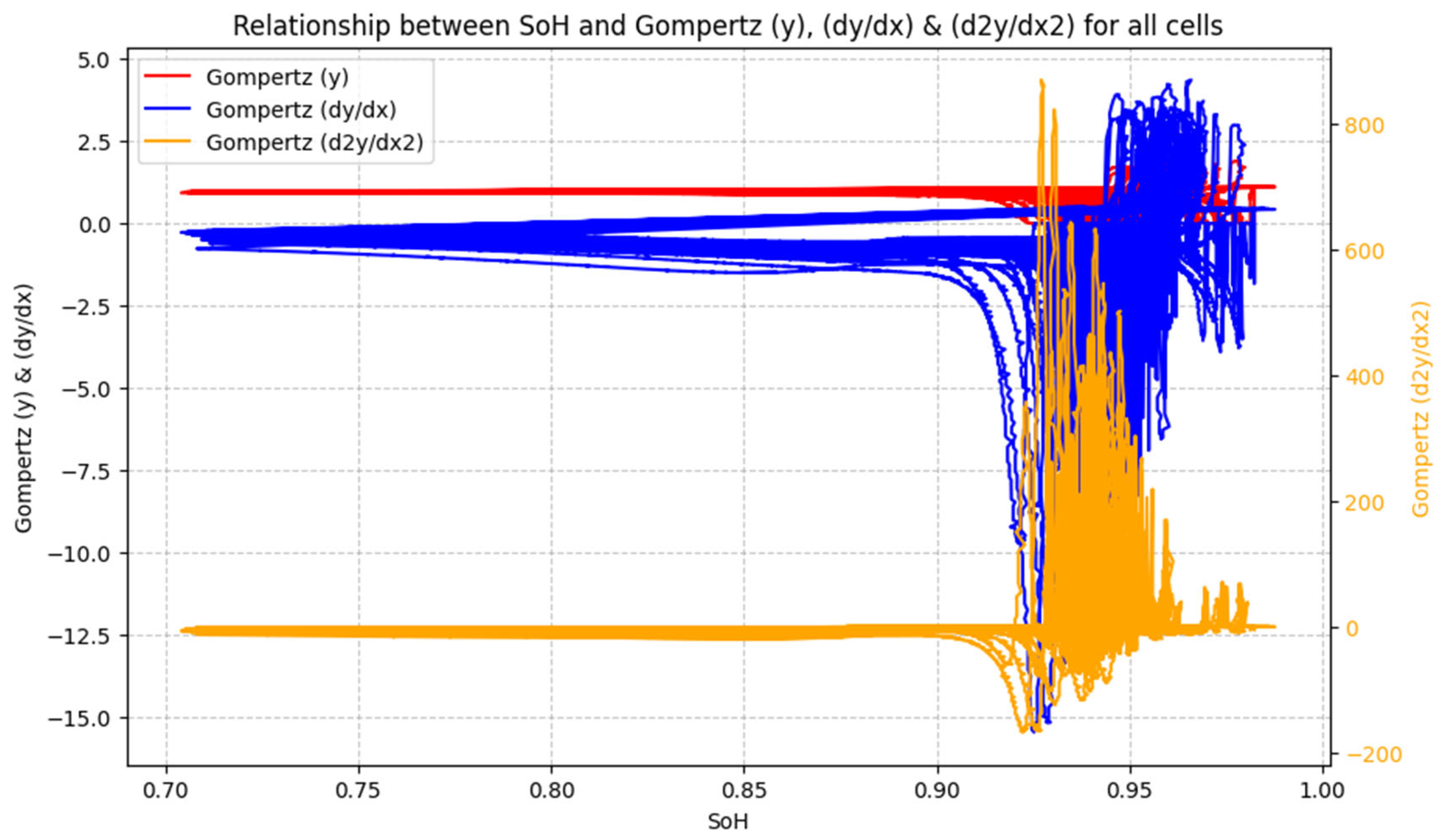
At SoH values between 0.90 and 1.0, and exhibit high variability while below 0.9 SoH, the curves smoothen out showing how in the initial SoH stages it is far harder to predict RUL and SoH based on than in the latter stages, 0.9 SoH to 0.7 SoH.
Appendix B
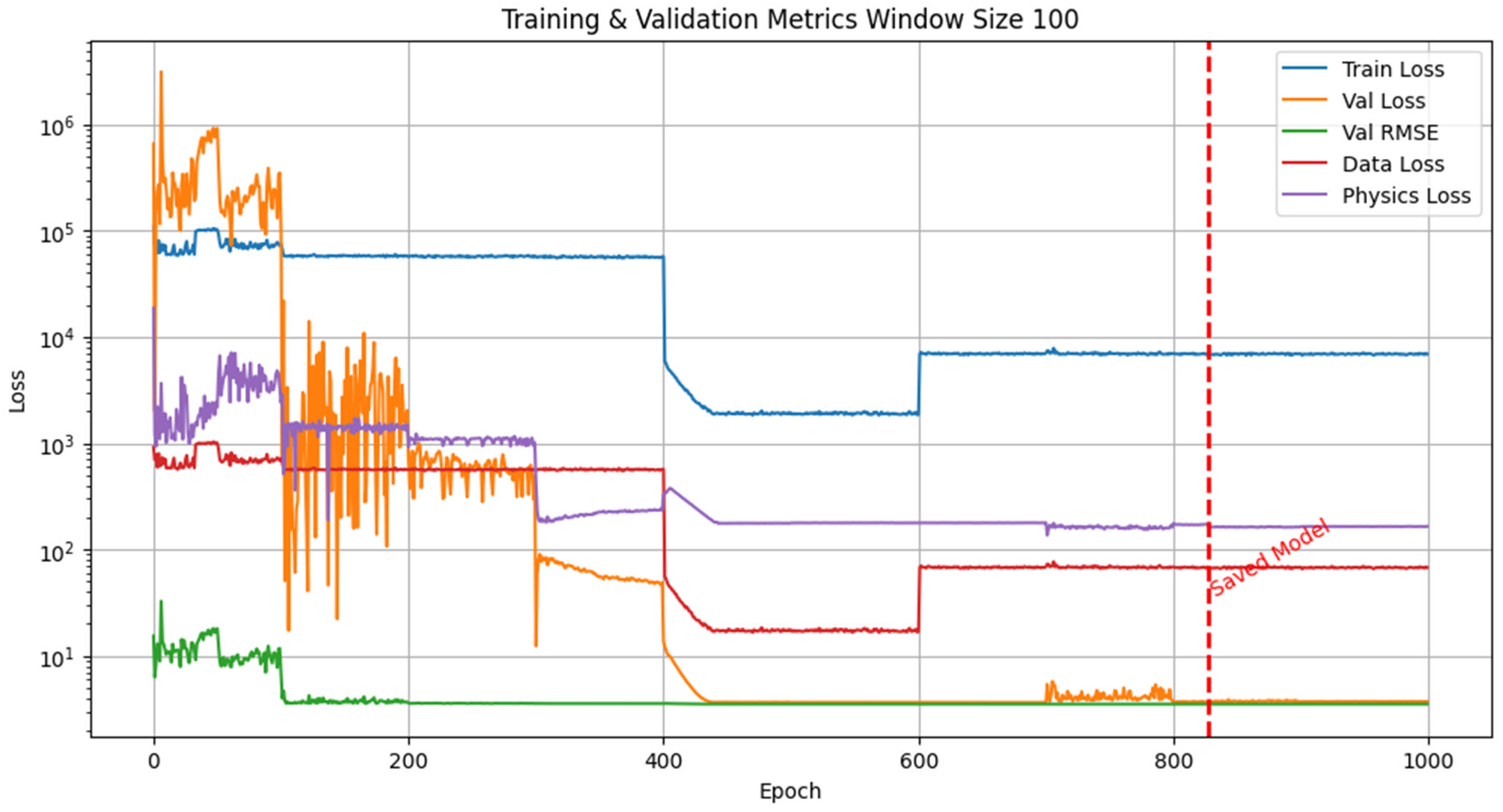
The figures below represent the training and validation metrics of GILSTM2 when the ablation study was conducted. They show the curriculum learning strategy, the effect of removing parts of the physics loss function and that the validation RMSE did not improve past 2.52.
Figure A2.
Model trained using
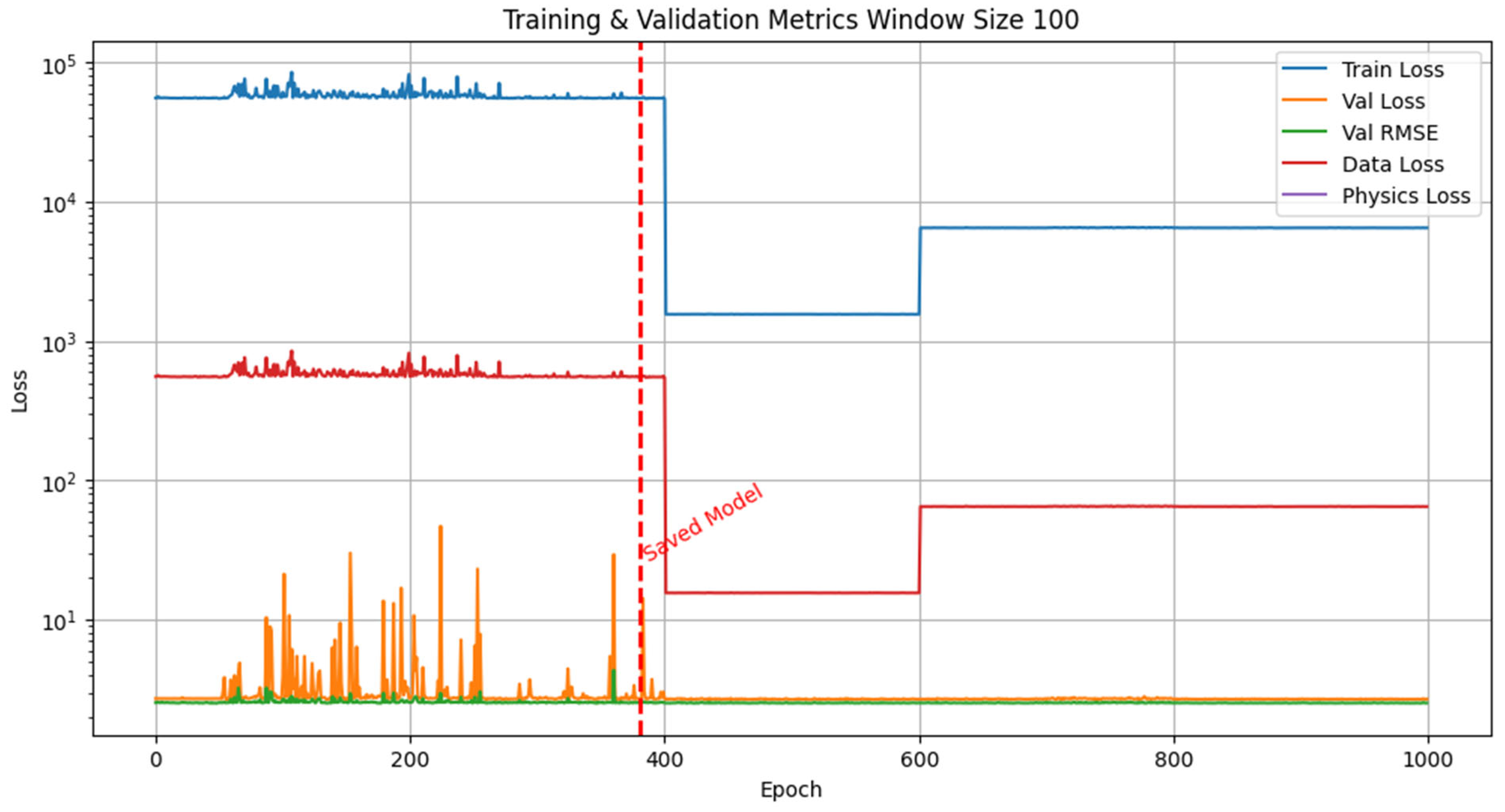
Figure A3.
Model trained using
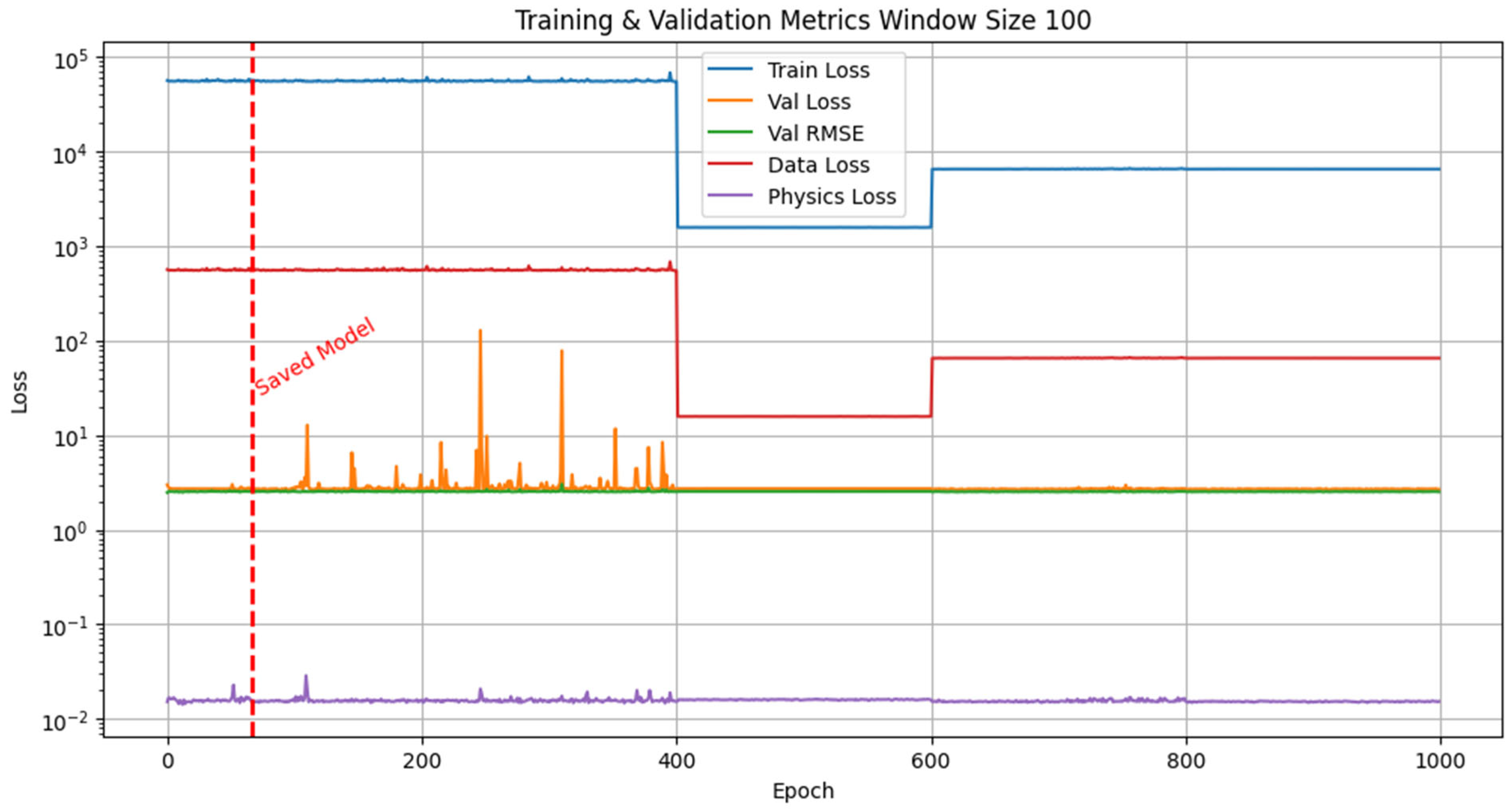
Figure A4.
Model trained using
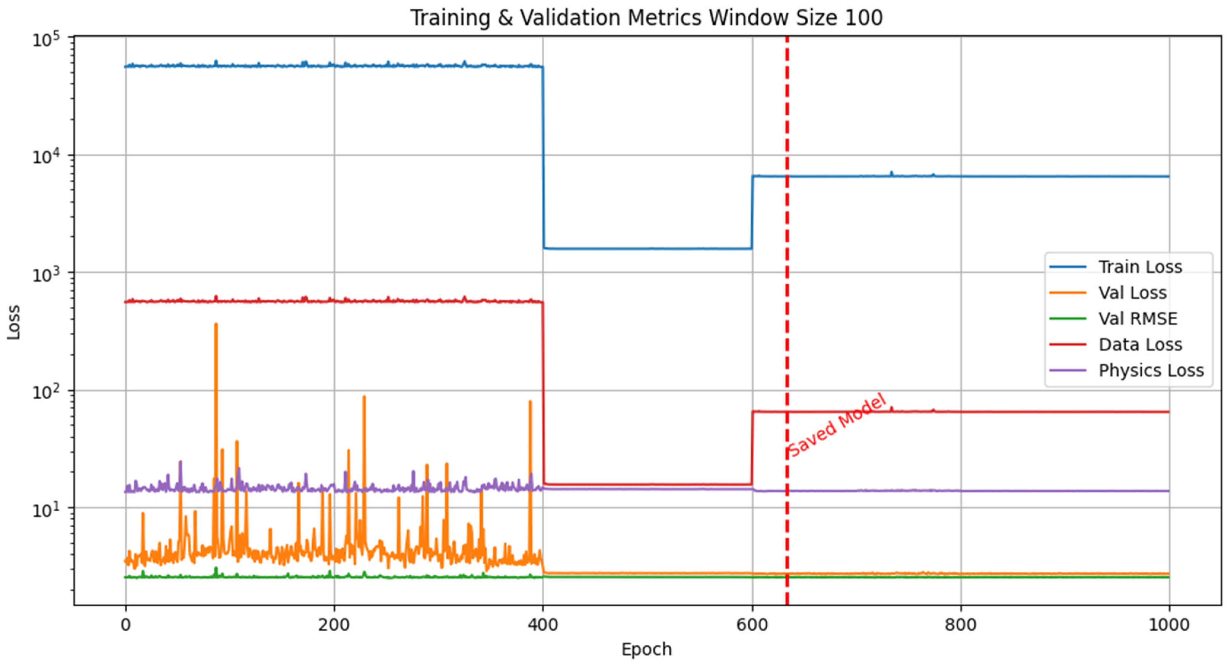
Figure A5.
GILSTM trained only on data with SoH less than 0.85 (stable data).
References
- Dowejko, J.; Jaworski, J. Beyond Traditional Grid: A Novel Quantitative Framework for Assessing Automation’s Impact on System Average Interruption Duration Index and System Average Interruption Frequency Index. Energies 2025, 18, 2671. [Google Scholar] [CrossRef] [Scilit]
- Hu, Y.; Armada, M.; Jesús Sánchez, M. Potential Utilization of Battery Energy Storage Systems (BESS) in the Major European Electricity Markets. Appl. Energy 2022, 322, 119512. [Google Scholar] [CrossRef] [Scilit]
- Shafiei, K.; Zadeh, S.G.; Hagh, M.T. Planning for a Network System with Renewable Resources and Battery Energy Storage, Focused on Enhancing Resilience. J. Energy Storage 2024, 87, 111339. [Google Scholar] [CrossRef] [Scilit]
- Ahmed, K.M.U.; Alvarez, M.; Bollen, M.H.J. Reliability Analysis of Internal Power Supply Architecture of Data Centers in Terms of Power Losses. Electr. Power Syst. Res. 2021, 193, 107025. [Google Scholar] [CrossRef] [Scilit]
- Soubhi Hussein, Y.; Alrashd, M.; Saeed Alabed, A.; Zraiqat, A. Data Centre Infrastructure: Power Efficiency and Protection. In Latest Advances and New Visions of Ontology in Information Science; SaberiKamarposhti, M., Sahlabadi, M., Eds.; IntechOpen: London, UK, 2023. [Google Scholar]
- Lin, L.; Wijayawardana, R.; Rao, V.; Nguyen, H.; Gnibga, E.W.; Chien, A.A. Exploding AI Power Use: An Opportunity to Rethink Grid Planning and Management. In Proceedings of the 15th ACM International Conference on Future and Sustainable Energy Systems; ACM: Singapore, 2024; pp. 434–441. [Google Scholar]
- Serban, E.; Ordonez, M.; Pondiche, C. Voltage and Frequency Grid Support Strategies Beyond Standards. IEEE Trans. Power Electron. 2017, 32, 298–309. [Google Scholar] [CrossRef] [Scilit]
- Feng, X.; Ren, D.; Ouyang, M. Safety of Lithium Battery Materials Chemistry. J. Mater. Chem. A 2023, 11, 25236–25246. [Google Scholar] [CrossRef] [Scilit]
- Wei, G.; Huang, R.; Zhang, G.; Jiang, B.; Zhu, J.; Guo, Y.; Han, G.; Wei, X.; Dai, H. A Comprehensive Insight into the Thermal Runaway Issues in the View of Lithium-Ion Battery Intrinsic Safety Performance and Venting Gas Explosion Hazards. Appl. Energy 2023, 349, 121651. [Google Scholar] [CrossRef] [Scilit]
- Li, W.; Wang, H.; Zhang, Y.; Ouyang, M. Flammability Characteristics of the Battery Vent Gas: A Case of NCA and LFP Lithium-Ion Batteries during External Heating Abuse. J. Energy Storage 2019, 24, 100775. [Google Scholar] [CrossRef] [Scilit]
- Brand, M.; Gläser, S.; Geder, J.; Menacher, S.; Obpacher, S.; Jossen, A.; Quinger, D. Electrical Safety of Commercial Li-Ion Cells Based on NMC and NCA Technology Compared to LFP Technology. In Proceedings of the 2013 World Electric Vehicle Symposium and Exhibition (EVS27); IEEE: Piscataway, NJ, USA, 2013; pp. 1–9. [Google Scholar]
- Watt Happens Next: LFP Is Taking Over—Here’s Why It Matters. Available online: https://erv.io/knowledge_hub/watt-happens-next-lfp-is-taking-over-heres-why-it-matters/ (accessed on 14 April 2025).
- Mou, J.; Yang, Q.; Tang, Y.; Liu, Y.; Li, J.; Yu, C. Prediction of the Remaining Useful Life of Lithium-Ion Batteries Based on the 1D CNN-BLSTM Neural Network. Batteries 2024, 10, 152. [Google Scholar] [CrossRef] [Scilit]
- Zhang, Y.; Song, W.; Lin, S.; Feng, Z. A Novel Model of the Initial State of Charge Estimation for LiFePO4 Batteries. J. Power Sources 2014, 248, 1028–1033. [Google Scholar] [CrossRef] [Scilit]
- Feng, F.; Lu, R.; Zhu, C. A Combined State of Charge Estimation Method for Lithium-Ion Batteries Used in a Wide Ambient Temperature Range. Energies 2014, 7, 3004–3032. [Google Scholar] [CrossRef] [Scilit]
- Gailani, A.; Mokidm, R.; El-Dalahmeh, M.; El-Dalahmeh, M.; Al-Greer, M. Analysis of Lithium-Ion Battery Cells Degradation Based on Different Manufacturers. In 2020 55th International Universities Power Engineering Conference (UPEC); IEEE: Piscataway, NJ, USA, 2020. [Google Scholar]
- Sayyad, S.; Kumar, S.; Bongale, A.; Kamat, P.; Patil, S.; Kotecha, K. Data-Driven Remaining Useful Life Estimation for Milling Process: Sensors, Algorithms, Datasets, and Future Directions. IEEE Access 2021, 9, 110255–110286. [Google Scholar] [CrossRef] [Scilit]
- Zhou, Y.; Liu, C.; Yu, X.; Liu, B.; Quan, Y. Tool Wear Mechanism, Monitoring and Remaining Useful Life (RUL) Technology Based on Big Data: A Review. SN Appl. Sci. 2022, 4, 232. [Google Scholar] [CrossRef] [Scilit]
- Ayob, A.; Ansari, S.; Lipu, M.S.H.; Hussain, A.; Saad, M.H.M. SOC, SOH and RUL Estimation for Supercapacitor Management System: Methods, Implementation Factors, Limitations and Future Research Improvements. Batteries 2022, 8, 189. [Google Scholar] [CrossRef] [Scilit]
- Shekhar, R. Comprehensive Compilation of Energy Units and Conversion Factors: A Technical Reference. ResearchGate 2024. Available online: https://www.researchgate.net/publication/383741261_Comprehensive_Compilation_of_Energy_Units_and_Conversion_Factors_A_Technical_Reference (accessed on 21 April 2026).
- Lashway, C.R.; Mohammed, O.A. Adaptive Battery Management and Parameter Estimation Through Physics-Based Modeling and Experimental Verification. IEEE Trans. Transp. Electrif. 2016, 2, 454–464. [Google Scholar] [CrossRef] [Scilit]
- Sundén, B. Chapter 6—Thermal Management of Batteries. In Hydrogen, Batteries and Fuel Cells; Sundén, B., Ed.; Academic Press: Cambridge, MA, USA, 2019; pp. 93–110. [Google Scholar]
- Kong, X.; Bonakdarpour, A.; Wetton, B.T.; Wilkinson, D.P.; Gopaluni, B. State of Health Estimation for Lithium-Ion Batteries. IFAC-PapersOnLine 2018, 51, 667–671. [Google Scholar] [CrossRef] [Scilit]
- Xiong, R.; He, H.; Sun, F.; Zhao, K. Evaluation on State of Charge Estimation of Batteries With Adaptive Extended Kalman Filter by Experiment Approach. IEEE Trans. Veh. Technol. 2013, 62, 108–117. [Google Scholar] [CrossRef] [Scilit]
- Manmi, K.; Tuchel, M.; Kendrick, E.; Brosa Planella, F. A Comparison of Standard SEI Growth Models in the Context of Battery Formation. J. Electrochem. Soc. 2024, 171, 100530. [Google Scholar] [CrossRef] [Scilit]
- Adenusi, H.; Chass, G.A.; Passerini, S.; Tian, K.V.; Chen, G. Lithium Batteries and the Solid Electrolyte Interphase (SEI)—Progress and Outlook. Adv. Energy Mater. 2023, 13, 2203307. [Google Scholar] [CrossRef] [Scilit]
- Frankenberger, M.; Trunk, M.; Seidlmayer, S.; Dinter, A.; Dittloff, J.; Werner, L.; Gernhäuser, R.; Revay, Z.; Märkisch, B.; Gilles, R.; et al. SEI Growth Impacts of Lamination, Formation and Cycling in Lithium Ion Batteries. Batteries 2020, 6, 21. [Google Scholar] [CrossRef] [Scilit]
- Hosseininasab, S.; Lin, C.; Pischinger, S.; Stapelbroek, M.; Vagnoni, G. State-of-Health Estimation of Lithium-Ion Batteries for Electrified Vehicles Using a Reduced-Order Electrochemical Model. J. Energy Storage 2022, 52, 104684. [Google Scholar] [CrossRef] [Scilit]
- Couto, L.D.; Capron, O.; Servotte, J.; Ponnette, R.; Mulder, G. Physics-Based Lifetime Modeling and Parameter Identification of Lithium-Ion Batteries under Various Degradation Conditions. J. Energy Storage 2025, 127, 116739. [Google Scholar] [CrossRef] [Scilit]
- Ma, G.; Xu, S.; Jiang, B.; Cheng, C.; Yang, X.; Shen, Y.; Yang, T.; Huang, Y.; Ding, H.; Yuan, Y. Real-Time Personalized Health Status Prediction of Lithium-Ion Batteries Using Deep Transfer Learning. Energy Environ. Sci. 2022, 15, 4083–4094. [Google Scholar] [CrossRef] [Scilit]
- Severson, K.A.; Attia, P.M.; Jin, N.; Perkins, N.; Jiang, B.; Yang, Z.; Chen, M.H.; Aykol, M.; Herring, P.K.; Fraggedakis, D.; et al. Data-Driven Prediction of Battery Cycle Life before Capacity Degradation. Nat. Energy 2019, 4, 383–391. [Google Scholar] [CrossRef] [Scilit]
- Catelani, M.; Ciani, L.; Fantacci, R.; Patrizi, G.; Picano, B. Remaining Useful Life Estimation for Prognostics of Lithium-Ion Batteries Based on Recurrent Neural Network. IEEE Trans. Instrum. Meas. 2021, 70, 3524611. [Google Scholar] [CrossRef] [Scilit]
- Feng, H.; Shi, G. SOH and RUL Prediction of Li-Ion Batteries Based on Improved Gaussian Process Regression. J. Power Electron. 2021, 21, 1845–1854. [Google Scholar] [CrossRef] [Scilit]
- Cheng, G.; Wang, X.; He, Y. Remaining Useful Life and State of Health Prediction for Lithium Batteries Based on Empirical Mode Decomposition and a Long and Short Memory Neural Network. Energy 2021, 232, 121022. [Google Scholar] [CrossRef] [Scilit]
- Ma, Y.; Yao, M.; Liu, H.; Tang, Z. State of Health Estimation and Remaining Useful Life Prediction for Lithium-Ion Batteries by Improved Particle Swarm Optimization-Back Propagation Neural Network. J. Energy Storage 2022, 52, 104750. [Google Scholar] [CrossRef] [Scilit]
- Wang, S.; Fan, Y.; Jin, S.; Takyi-Aninakwa, P.; Fernandez, C. Improved Anti-Noise Adaptive Long Short-Term Memory Neural Network Modeling for the Robust Remaining Useful Life Prediction of Lithium-Ion Batteries. Reliab. Eng. Syst. Saf. 2023, 230, 108920. [Google Scholar] [CrossRef] [Scilit]
- Li, Y.; Kang, L.; Wang, X.; Xie, D.; Wang, S. State of Health Prediction of Lithium-Ion Batteries Based on Dual-Time-Scale Self-Supervised Learning. Batteries 2025, 11, 302. [Google Scholar] [CrossRef] [Scilit]
- Li, X.; Wu, G.; Chang, F.; Xia, W.; Sun, S.; Shen, Y.; Li, X.; Wu, G.; Chang, F.; Xia, W.; et al. A Physics-Guided Transformer for Robust State of Charge Estimation in Aging Lithium-Ion Batteries. Batteries 2025, 11, 446. [Google Scholar] [CrossRef] [Scilit]
- Madani, S.S.; Shabeer, Y.; Fowler, M.; Panchal, S.; Chaoui, H.; Mekhilef, S.; Dou, S.X.; See, K. Artificial Intelligence and Digital Twin Technologies for Intelligent Lithium-Ion Battery Management Systems: A Comprehensive Review of State Estimation, Lifecycle Optimization, and Cloud-Edge Integration. Batteries 2025, 11, 298. [Google Scholar] [CrossRef] [Scilit]
- Zhang, H.; Gui, X.; Zheng, S.; Lu, Z.; Li, Y.; Bian, J. BatteryML: An Open-Source Platform for Machine Learning on Battery Degradation. arXiv 2024, arXiv:2310.14714. [Google Scholar]
- Winsor, C.P. The Gompertz Curve as a Growth Curve. Proc. Natl. Acad. Sci. USA 1932, 18, 1–8. [Google Scholar] [CrossRef] [Scilit]
- Yang, N.; Song, Z.; Hofmann, H.; Sun, J. Robust State of Health Estimation of Lithium-Ion Batteries Using Convolutional Neural Network and Random Forest. J. Energy Storage 2022, 48, 103857. [Google Scholar] [CrossRef] [Scilit]
- Che, Y.; Hu, X.; Lin, X.; Guo, J.; Teodorescu, R. Health Prognostics for Lithium-Ion Batteries: Mechanisms, Methods, and Prospects. Energy Environ. Sci. 2023, 16, 338–371. [Google Scholar] [CrossRef] [Scilit]
- Enuh, B.M. What Are Battery Management Systems and How Do They Impact Energy Storage Systems? Available online: https://www.azom.com/article.aspx?ArticleID=22797 (accessed on 3 March 2025).
- Ur Rehman, M.M.; Evzelman, M.; Hathaway, K.; Zane, R.; Plett, G.L.; Smith, K.; Wood, E.; Maksimovic, D. Modular Approach for Continuous Cell-Level Balancing to Improve Performance of Large Battery Packs. In Proceedings of the 2014 IEEE Energy Conversion Congress and Exposition (ECCE); IEEE: Piscataway, NJ, USA, 2014; pp. 4327–4334. [Google Scholar]
- Bašić, H.; Bobanac, V.; Pandžić, H. Determination of Lithium-Ion Battery Capacity for Practical Applications. Batteries 2023, 9, 459. [Google Scholar] [CrossRef] [Scilit]
- Hochreiter, S.; Schmidhuber, J. Long Short-Term Memory. Neural Comput. 1997, 9, 1735–1780. [Google Scholar] [CrossRef] [Scilit] [PubMed]
- Kingma, D.P.; Ba, J. Adam: A Method for Stochastic Optimization. arXiv 2017, arXiv:1412.6980. [Google Scholar] [CrossRef] [Scilit]
- Soviany, P.; Ionescu, R.T.; Rota, P.; Sebe, N. Curriculum Learning: A Survey. Int. J. Comput. Vis. 2022, 130, 1526–1565. [Google Scholar] [CrossRef] [Scilit]
- Raissi, M.; Perdikaris, P.; Karniadakis, G.E. Physics-Informed Neural Networks: A Deep Learning Framework for Solving Forward and Inverse Problems Involving Nonlinear Partial Differential Equations. J. Comput. Phys. 2019, 378, 686–707. [Google Scholar] [CrossRef] [Scilit]
- Zhang, H.; Li, Y.; Zheng, S.; Lu, Z.; Gui, X.; Xu, W.; Bian, J. Accurate Battery Lifetime Prediction across Diverse Aging Conditions with Deep Learning. arXiv 2023, arXiv:2310.05052. [Google Scholar] [CrossRef] [Scilit]

Disclaimer/Publisher’s Note: The statements, opinions and data contained in all publications are solely those of the individual author(s) and contributor(s) and not of MDPI and/or the editor(s). MDPI and/or the editor(s) disclaim responsibility for any injury to people or property resulting from any ideas, methods, instructions or products referred to in the content. |
© 2026 by the authors. Licensee MDPI, Basel, Switzerland. This article is an open access article distributed under the terms and conditions of the Creative Commons Attribution (CC BY) license.