Early Remaining Useful Life Prediction for Lithium-Ion Batteries Using a Gaussian Process Regression Model Based on Degradation Pattern Recognition ^†

Abstract

Lithium-ion batteries experience nonlinear degradation characteristics during long-term operation. Accurate estimation of their remaining useful life (RUL) is of significant importance for early fault diagnosis and residual value evaluation. However, existing RUL prediction approaches often suffer from limited accuracy and insufficient specificity. To address these limitations, this study proposes an RUL prediction methodology based on Gaussian process regression, which incorporates degradation pattern recognition and auxiliary features derived from knee points. First, 9 health-related features are extracted from the first 100 charge/discharge cycles of the battery. Based on these extracted features, clustering and classification techniques are employed to categorize the batteries into three distinct degradation patterns. Moreover, feature importance is assessed to identify and eliminate redundant indicators, thereby enhancing the relevance of the feature set for prediction. Subsequently, for each degradation pattern, GPR-based models with composite kernel functions are constructed by integrating knee point positions and their corresponding slopes. The model hyperparameters are further optimized through the particle swarm optimization (PSO) algorithm to improve the adaptability and generalization capability of the predictive models. Experimental results demonstrate that the proposed method achieves a high level of predictive accuracy, with an overall mean absolute percentage error (MAPE) of approximately 8.70%. Furthermore, compared with conventional prediction methods, the proposed approach exhibits superior performance and can serve as an effective evaluation tool for diverse application scenarios, including lithium-ion battery health monitoring, early prognostics, and echelon utilization.

1. Introduction

New energy vehicles, consistent with the sustainable development concept of modern society, are gaining increasing popularity. Lithium-ion batteries (LIBs) are widely used in new energy vehicles due to their high energy density, fast charging capability, and low self-discharge rate [1,2,3]. However, it is a dynamic and nonlinear fading system with complex internal mechanisms. As charge/discharge cycles increase, physicochemical reactions will lead to loss of lithium-ion inventory (LLI) and loss of anode/cathode active materials (LAMs) [4,5], thus leading to battery performance degradation. When the battery’s capacity decays to 80% [6] of initial capacity or internal resistance increases to 200% of initial resistance [7,8], the battery reaches its end of life (EOL) and may suffer severe failures such as accelerated attenuation and unexpected downtime [9,10]. At this point, the battery should be replaced to guarantee the expected performance and safety. In addition, retired batteries may still have a high residual value and can be utilized in applications where high performance is not critical, such as energy storage and power plants [11,12]. Hence, predicting battery cycle life before severe degradation is of vital importance for early health diagnosis, timely safety maintenance, residual value assessment, and regulation of secondary usage.

Battery life prediction methods are typically classified into model-based, data-driven, and hybrid approaches. Among them, model-based methods seek to develop a mathematical model that captures the degradation trajectory by leveraging the inherent battery dynamics [13], and various models can be used, including the electrochemical model [14], equivalent circuit model (ECM) [15], and empirical model [16]. An electrochemical model accurately describes the physicochemical phenomena such as the intercalation and deintercalation of lithium ions between the anode and cathode and the electrochemical reactions on the surface of the electrodes. The P2D model is a commonly used electrochemical model. Ramadesigan et al. [17] reconstructed a P2D model for battery life prediction, which accurately and effectively predicted the future capacity degradation of Li-ion batteries by inferring the variation of battery kinetic parameters. An ECM is constructed by assembling circuit elements in a manner that replicates the electrical behavior exhibited by the battery. [13]. Guha et al. [18] presented an approach for the estimation of the electrochemical impedance spectrum (EIS) of lithium-ion batteries based on a fractional-order equivalent circuit model (FOECM) and then predicted the lifetime based on EIS data. An empirical model employs various regression techniques to capture the fading trend or formulates suitable empirical expressions to characterize and predict the degradation state of the battery [13]. Micea et al. [19] developed a quadratic polynomial regression model to fit the degradation trend of Ni-MH batteries under low currents. The mechanistic model is more precise but highly complex; therefore, the parameter identification for a mechanistic model is challenging and time-consuming [20]. These models require a deep understanding of battery electrochemistry and often involve solving coupled nonlinear equations, which leads to high computational costs [13]. Moreover, many model parameters, such as diffusion coefficients or interface resistances, are difficult to measure directly and may vary with operating conditions, making calibration both difficult and resource-intensive. Mechanistic models are also sensitive to initial and boundary conditions, and small input uncertainties can significantly affect prediction accuracy. Empirical models are relatively simple, as they omit the complex internal dynamics of the battery. Nevertheless, their parameters generally lack physical interpretability, and such models often exhibit limited generalization capability across varying operating conditions. They are typically fitted to specific datasets, so their performance may degrade when applied to different operating conditions or battery types, i.e., low generalization ability [13]. In addition, empirical models often require large amounts of data to maintain accuracy, and their predictive capability is limited when data is scarce or noisy.

Data-driven approaches attempt to extract hidden relationships from battery data and predict the remaining useful life (RUL) without a battery mathematical model, which is feasible and practical when a large amount of data is available [13]. These methods bypass complex physical modeling by learning degradation patterns directly from external battery data such as voltage, current, and temperature, which avoid the need for detailed electrochemical modeling and complex parameter identification, thereby significantly reducing modeling complexity and computational cost [7]. With advances in artificial intelligence, especially large-scale models, data-driven approaches can approximate internal behaviors with reduced computational cost and minimal expert knowledge, making them suitable for real-time and scalable applications. Commonly used machine learning algorithms for RUL prediction include relevance vector machine (RVM) [21,22], support vector machine (SVM) [23,24], Gaussian process regression (GPR) [25,26], long short-term memory (LSTM) [27,28], etc. Wang et al. [23] extracted features from temperature and energy efficiency and predict battery life with an SVM model. Ren et al. [29] proposed a battery RUL prediction model based on a convolutional neural network (CNN) and LSTM, in which a CNN is used to extract hidden information from raw data, and an LSTM is used to process time series information. Jia et al. [25] extracted indirect health indicators and synergistically estimated the state of health (SOH) and battery lifetime by combining GPR and probabilistic prediction methods. The performance of data-driven methods significantly depends on the data quality and model generalization. In addition, the choice of hyperparameters in machine learning algorithms is also vital [28]. When the algorithm has a large number of hyperparameters to optimize, it may run inefficiently and also require a large search space.

In recent years, hybrid approaches that integrate model-based and data-driven methodologies have emerged, aiming to leverage the complementary advantages inherent in each approach. Li et al. [30] integrated the SVM with PF for battery life prediction, where PF was used to relocate particles and update the capacity estimation. However, combining multiple methods makes the model parameters more complex, leading to unstable predictions. Hence, the data-driven technique for lithium-ion battery life prediction remains the research focus [26].

Most existing data-driven models require 40~70% of the entire aging data to generate precise prediction results, which makes it challenging to achieve the battery early life prediction [31]. Early life prediction only employs a small amount of early cycle data to realize the RUL prediction, which can largely reduce battery data measurement, improve the efficiency of battery safety maintenance, and be significant in preventing unexpected LIB failure. However, predicting the degradation patterns and battery life at an early stage is still a challenging task. Early life prediction requires proper health feature extraction and prediction methods. The current early prediction method of battery life can be divided into two categories: the first is based on time series, and the second is based on early degradation features. Severson et al. [32] employed machine-learning tools to simultaneously predict and classify battery cells in terms of their cycle life, utilizing discharge voltage curves obtained from early-stage cycles, which achieved a 9.1% test error. Tong et al. [31] combined adaptive dropout long short-term memory (ADLSTM) and Monte Carlo (MC) simulation, and proposed a lithium-ion battery life prediction model that can accurately achieve the early prediction with only 25% of the degradation data. The model based on early degradation features is the mainstream for early RUL prediction, which characterizes the early degradation process with several health features. Tang et al. [33] extracted the cycle-to-cycle changes in the capacity–voltage curves to capture potential indicators of battery aging and established a hybrid model of CNN and LSTM to construct a mapping between health features and battery life.

The above discussion summarizes several representative early lifespan prediction methods, each demonstrating superior performance under specific circumstances. However, the following issues remain to be solved among current lifetime prediction methodologies.

(1)

The insufficiently comprehensive feature extraction. Battery degradation influences the dynamic trajectories of various battery states, such as voltage, current, capacity, and others. This inspires researchers to perform lifetime predictions based on the variation in the above states. Existing battery early-life prediction methods tend to extract health features only from a direct or indirect aging physical quantity [34], which makes it difficult to characterize early decline comprehensively. For example, Yin et al. [35] focus on a single discharge-derived feature, i.e., average power, without considering charging-phase information or a broader set of health indicators, which may limit the richness of the feature space used for life prediction.

(2)

The empirically determined machine learning hyperparameters. The data-driven model’s parameters are also directly assigned by experience without optimization, which may lead to the degradation of battery early life prediction capability. This approach is highly dependent on trial and error and expert intuition, which can be both time-consuming and inconsistent across datasets or tasks. Moreover, without systematic optimization, models are less likely to reach their full predictive potential, and the reproducibility of results may suffer due to the lack of standardized tuning procedures.

(3)

The interference between batteries with different degradation modes. Many existing studies apply machine learning models directly to the full dataset without performing degradation mode classification or clustering [36,37]. However, such an approach overlooks the inherent heterogeneity in battery aging behaviors arising from variations in usage conditions, manufacturing inconsistencies, or operational environments. Without separating different degradation patterns, the learned model tends to average across distinct behaviors, potentially masking important trends and leading to degraded predictive accuracy and generalization performance. Batteries with large differences in lifespan may have differences in degradation mechanisms and interfere with each other in machine learning.

In response to the above existing problems with early prediction models, this study proposes an early RUL prediction method for lithium-ion using a PSO-GPR model based on degradation pattern recognition and supplementary features from knee points. In our previous work, presented in ITEC Asia-Pacific 2024, Xi’an [38], the basic framework of PSO-GPR was initially introduced and performed with the MIT–Stanford dataset. This work offers significant contributions and extensions. Specifically, a total of nine battery degradation features which are divides into four types are extracted from the battery’s early charging/discharging process, and the batteries are recognized as three different degradation patterns. Then, early life prediction models based on GPR with composite kernel functions and feature engineering are established, and the particle swarm optimization algorithm is employed to adjust the hyperparameters to improve the model adaptiveness. The key contributions of this work are outlined as follows:

• The early aging of batteries in different life intervals may behave differently. To make the life prediction more targeted towards similar types, degradation pattern recognition was considered in advance. This prevents short-life batteries from being influenced by long-life batteries.
• Considering the influence of nonlinear aging on the lifetime, based on the correlation between the knee point and the EOL cycle, the predicted knee point and knee slope are innovatively used as supplementary features for the lifetime prediction, which improves the prediction accuracy of RUL.
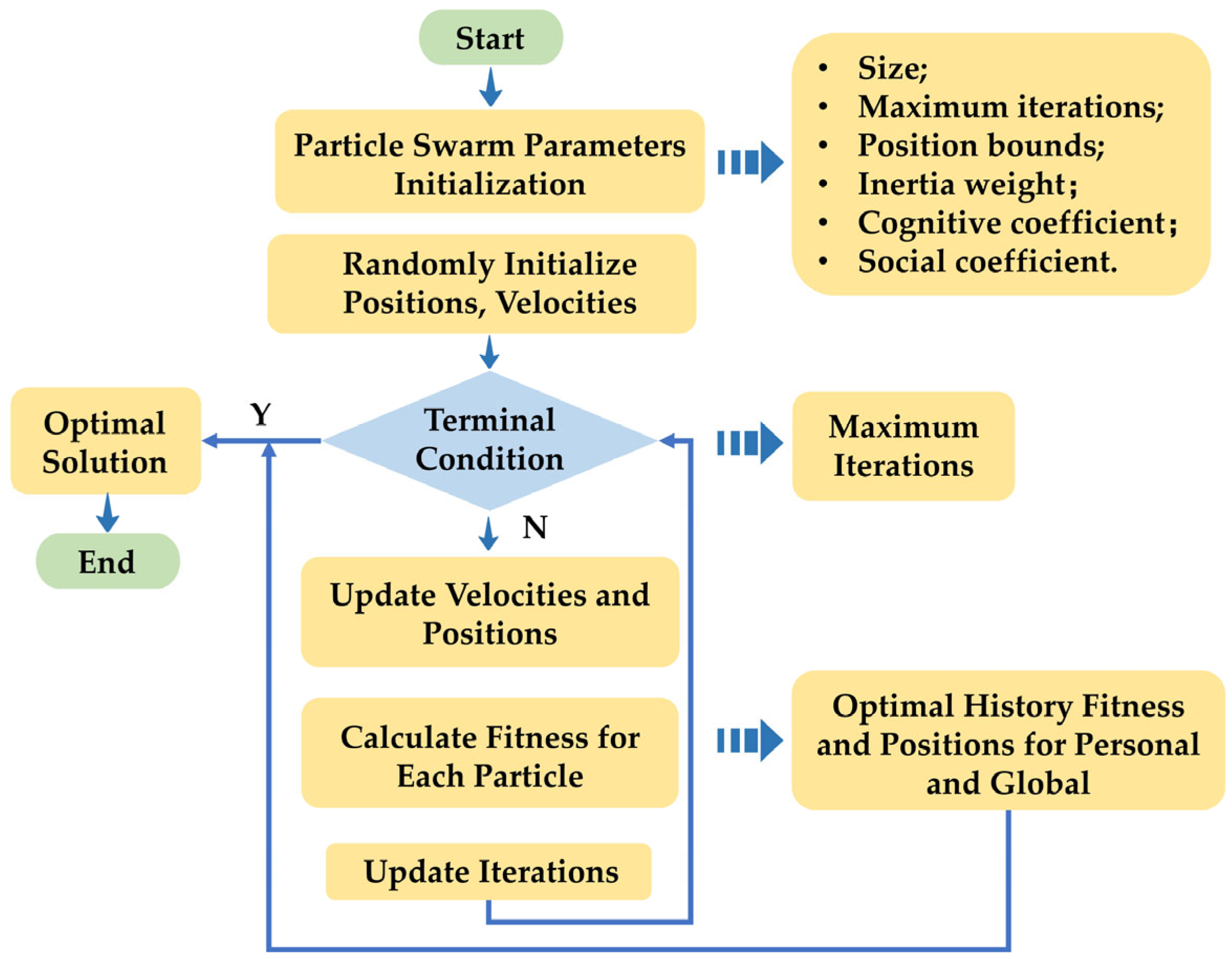
• To determine the hyperparameters of the composite kernel function in the GPR model, the particle swarm optimization algorithm was employed to achieve parameter self-tuning and enhance the adaptability of the prediction model.

The remaining part of the article proceeds as follows. Section 2 presents the battery degradation dataset employed in this study, along with the feature extraction and the methodology for degradation pattern recognition. Feature engineering and identification of the supplementary features related to the knee points are achieved in Section 3. Section 4 presents the framework and details of the proposed data-driven approach for battery early cycle life prediction based on PSO-GPR. Then, the experimental results of the proposed method are presented, and the model accuracy compared with other models is analyzed in Section 5. Finally, Section 6 summarizes the outlook and the limitations of this research and then gives the conclusion in Section 7.

2. Battery Dataset, Feature Extraction, and Degradation Pattern Recognition

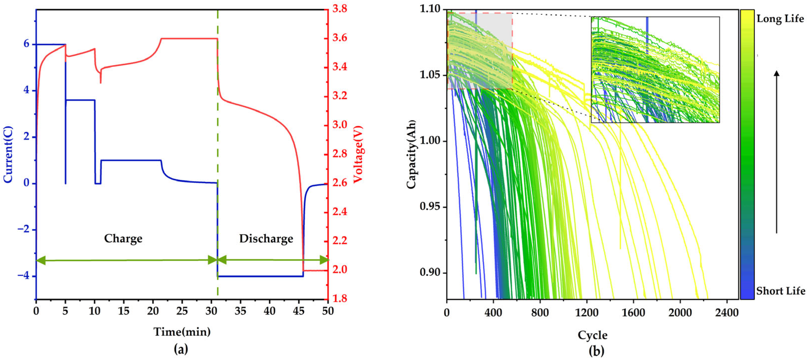
2.1. The Battery Aging Dataset

This study utilizes the publicly available MIT–Stanford lithium-ion battery dataset [32], which comprises 124 commercial phosphate/graphite cells (A123 Systems, model APR18650M1A). These cells have a nominal capacity of 1.1 Ah, with upper and lower cut-off voltage at 3.6 V and 2.0 V, respectively. A total of 72 distinct fast-charging protocols were employed to charge the batteries, followed by a constant current discharge at a rate of 4C, as illustrated in Figure 1a. The cells were cycled under ambient conditions at a temperature of 30 °C until they reached EOL, defined by a capacity drop below 80% of the nominal value. The dataset primarily documents parameters such as internal resistance and charge/discharge capacity between cycles, along with detailed measurements of temperature, voltage, current, and capacity for each cycle.

As shown in Figure 1b, the cycle lifespans of the batteries show substantial variation due to the diversity in fast-charging strategies. In addition, during the initial phase of cycling, the cells exhibit similar performance, which makes it difficult to predict their future degradation trends. As a result, selecting appropriate early-cycle features is essential for evaluating the current life stage of the batteries.

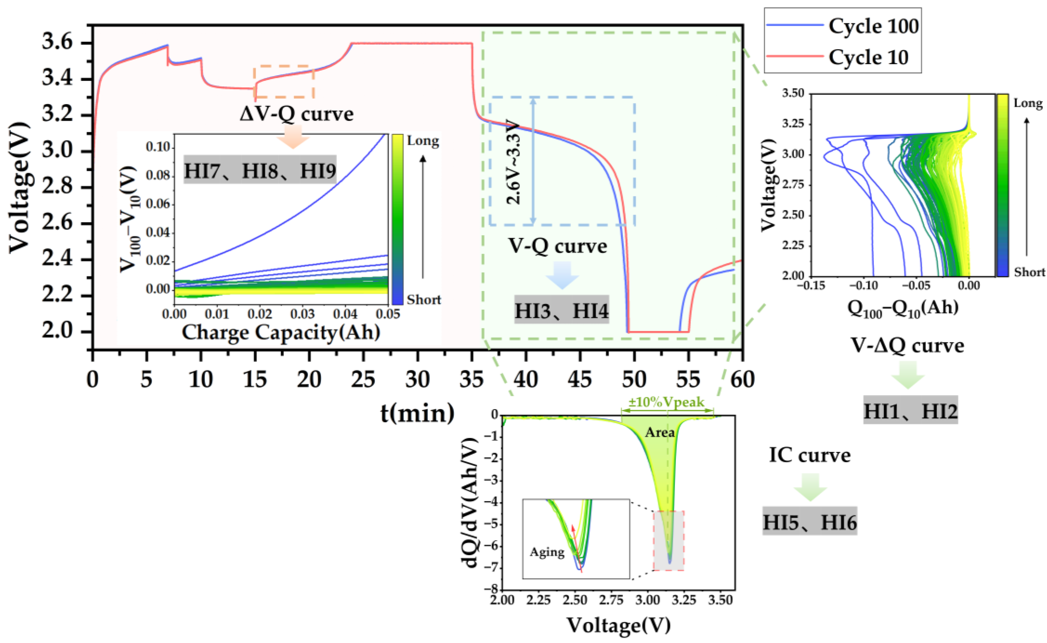
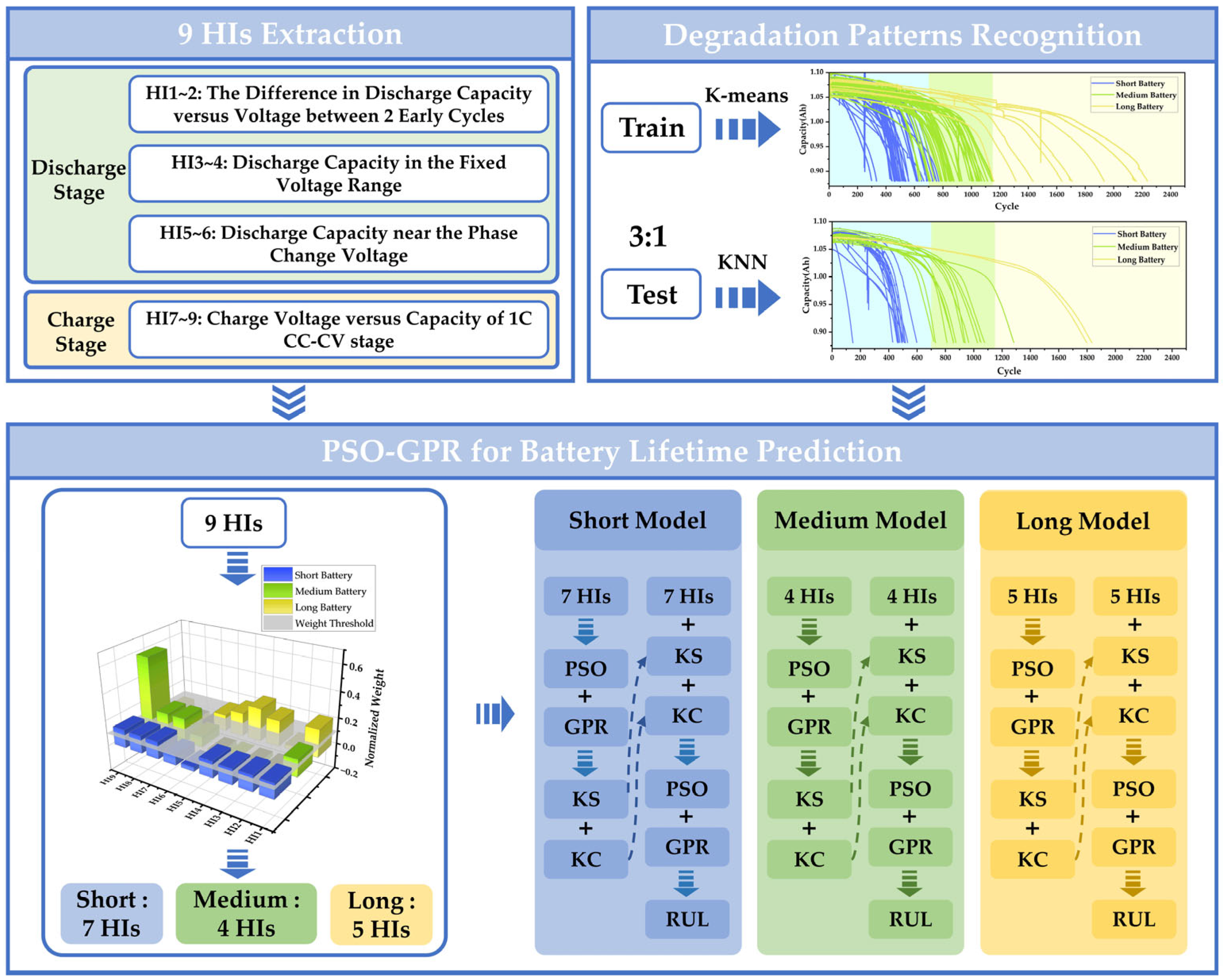
2.2. The Battery Health Indicator Extraction

Data-driven models utilize historical data to capture complex connections between features that are difficult to describe using mathematical formulas [34]. RUL prediction relies on health indicators (HIs) that characterize a battery’s ability to deliver the specified performance relative to a new battery and quantify its degradation state [13]. Feature extraction is performed by monitoring variations in multiple variables, such as temperature, voltage, capacity, etc., during the charge or discharge process. Additionally, the incremental capacity (IC) curve also provides useful details, as it reflects how much current the battery can deliver at a certain voltage, offering insights into RUL degradation. Similarly, the differential voltage (DV) curve is also available. As the battery ages, its charge and discharge capacity changes, which can indicate its current life stage. Meanwhile, voltage changes during these processes help describe its operating condition. Therefore, after analyzing the direct and indirect relationship between voltage and charge/discharge capacity in the early aging stage, a total of nine battery degradation features which are divides into four types are extracted from the aging process in this work. Additionally, the early-stage HIs not only reflect the battery’s current life stage but also help identify whether the battery is degrading quickly or slowly. These indicators are further applied in degradation pattern recognition, as described in Section 2.3. The general framework of the HIs is summarized in Figure 2. The extracted HIs are introduced as follows:

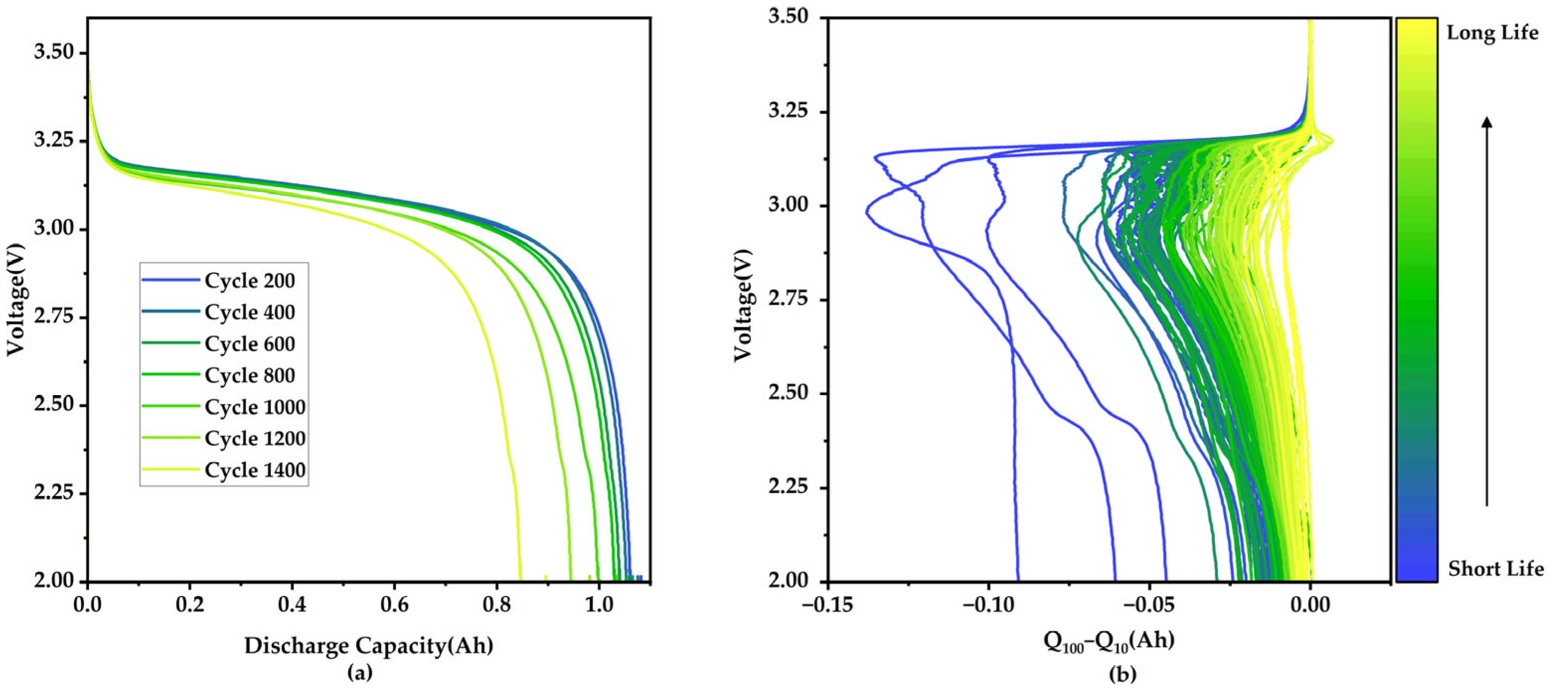
2.2.1. The Difference in Discharge Capacity Versus Voltage Between Two Early Cycles

It can be seen in Figure 3a that the discharge capacity curve gradually changes during battery aging. Thus, the cycle-to-cycle evolution of discharge capacity can be characterized as a health feature. The difference in discharge capacity curves between Cycle 100 and Cycle 10 is defined as Equation (1). Figure 3b illustrates that both the standard deviation and the peak values of these curves change in a monotonic way, which are extracted as HI1 and HI2.

$$\Delta Q_{100-10}\left(V\right)=Q_{100}\left(V\right)-Q_{10}\left(V\right)$$

(1)

where $Q_{100}\left(V\right)$ and $Q_{10}\left(V\right)$ are, respectively, the discharge capacity curves of Cycle 100 and Cycle 10.

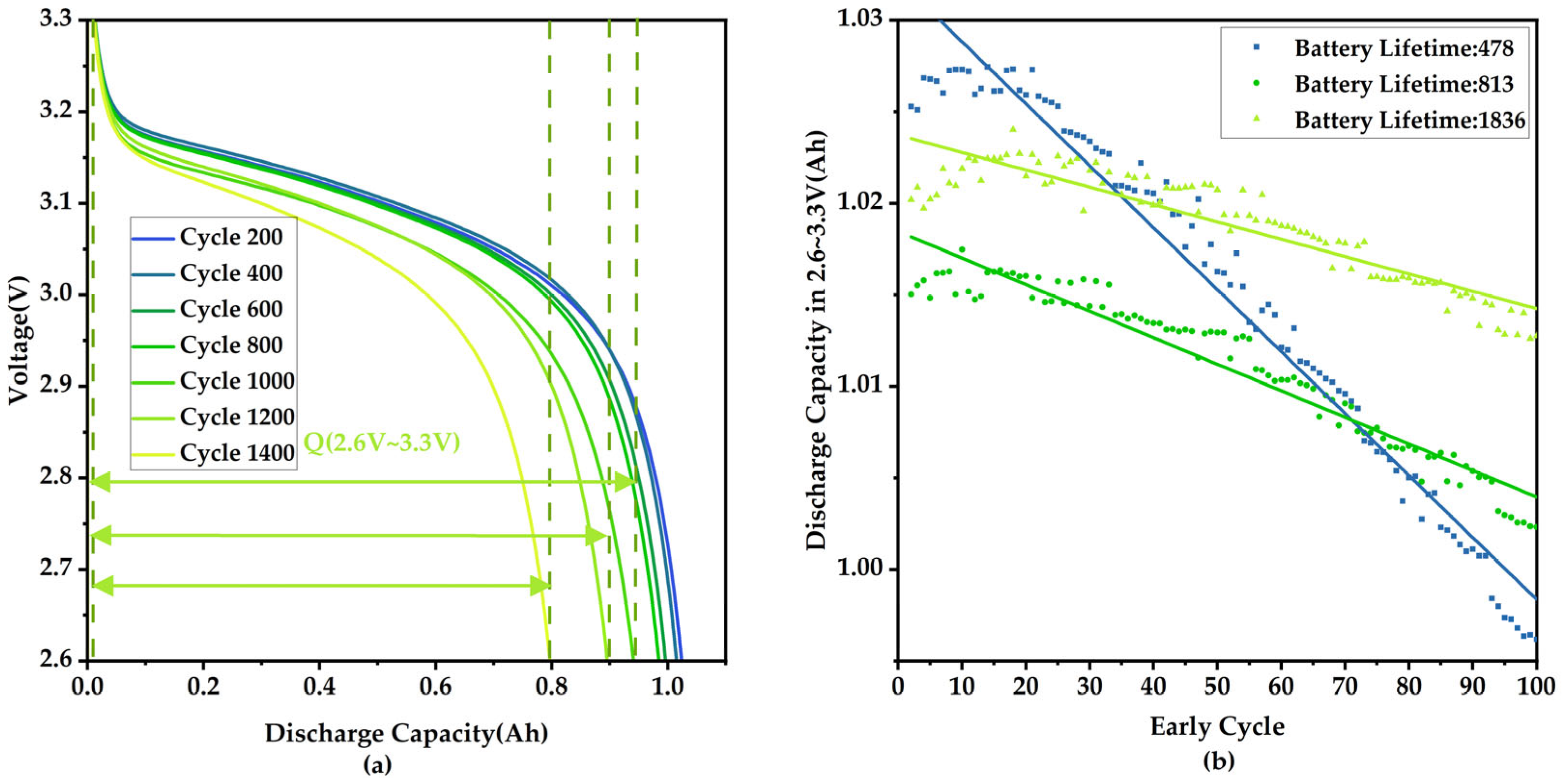
2.2.2. Discharge Capacity in the Fixed Voltage Range

Figure 3a also shows that the cumulative discharge capacity within each cycle gradually decreases as the battery ages. At the beginning (i.e., around 3.6 V) and at the end of the discharge (i.e., around 2 V), the cumulative discharge capacity shows minimal change. The discharge capacity within the main voltage range—where most of the change occurs—can effectively represent the battery’s performance in a specific cycle. The difference in discharge capacity in the fixed voltage range (2.6~3.3 V) between Cycle 100 and Cycle 10 is extracted as HI3, which is shown in Figure 4a. As shown in Figure 4b, the discharge capacity in this voltage range is approximately linearly related to early cycles (2nd~100th). The slope of the linear approximation of this curve is defined as HI4.

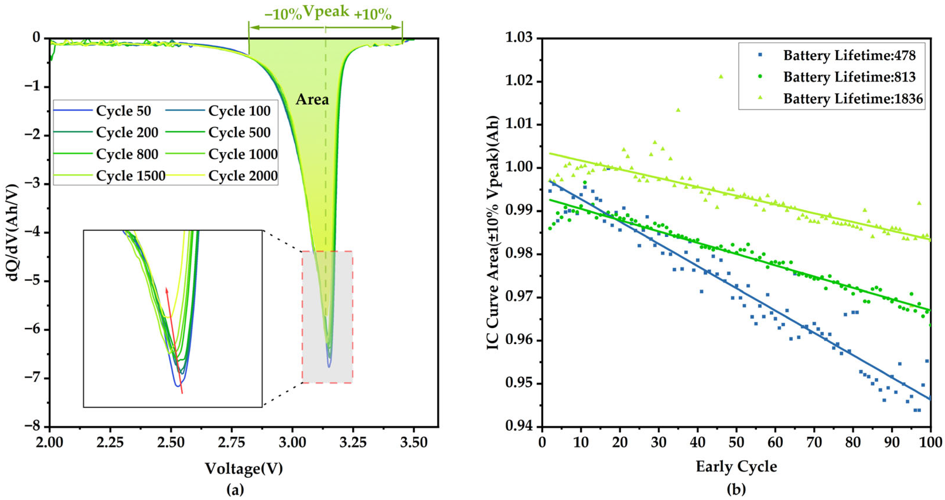
2.2.3. Discharge Capacity near the Phase Change Voltage

Figure 5a shows the IC curve of a specific battery during aging. The peak of the IC curve shifts slightly to the upper left. To amplify the change of the peak, the area near the peak of the IC curve (±10% peak voltage) is extracted, i.e., the discharge capacity near the phase change voltage, as shown in Figure 5a. The phase change voltage means the plateau voltage at which the positive electrodes of LiFePO₄ and FePO₄ of the LFP cell undergo a phase transition [39]. To exclude the interference of raw data noise on the IC curve, Gaussian smoothing is adopted, which retains the original features while denoising. The difference in this area between Cycle 100 and Cycle 10 is extracted as HI5. According to Figure 5b, this area shows a roughly linear relationship with early cycles (2nd~100th). We define the slope of the linear approximation of this curve as HI6.

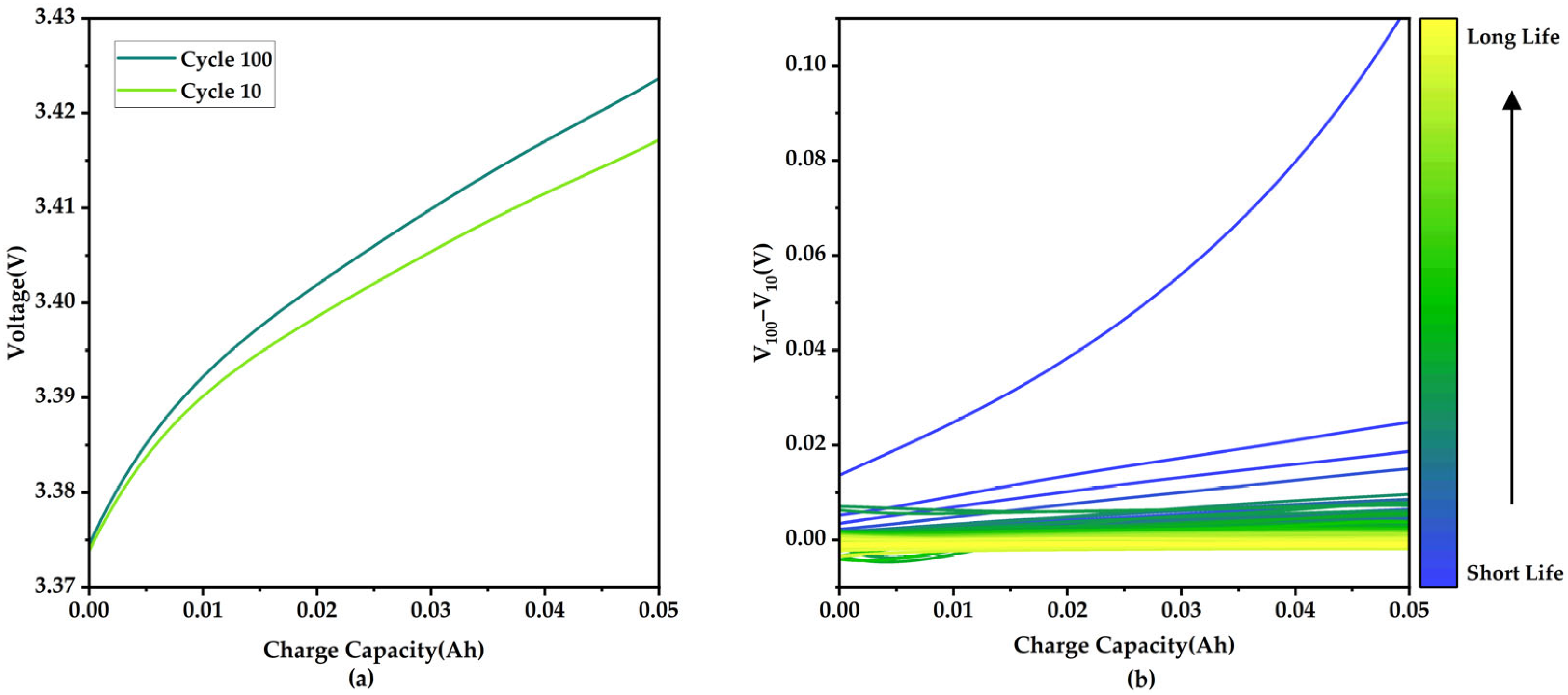
2.2.4. Charge Capacity of 1C CC-CV Stage

To alleviate users’ mileage anxiety, the traditional CC-CV charging policy has been gradually replaced by the multistep fast charging strategy. The MIT–Stanford dataset used in this research adopts the multistep fast-charging strategy, and the common point of all batteries is that they are charged with 1C CC-CV after 80% SOC. Therefore, this stage can be considered to extract the health features. Figure 6a represents the voltage change when the charging capacity of this stage changes from 0 to 0.05 Ah under Cycle 10 and Cycle 100 for one battery, and it can be found that the voltage varies with aging. On this basis, the difference of V₁₀₀−V₁₀ can be calculated. Figure 6b shows that there is a significant relationship between this difference and battery lifetime. Further, the mean, maximum, and variance of this curve are extracted as HI7, HI8, and HI9.

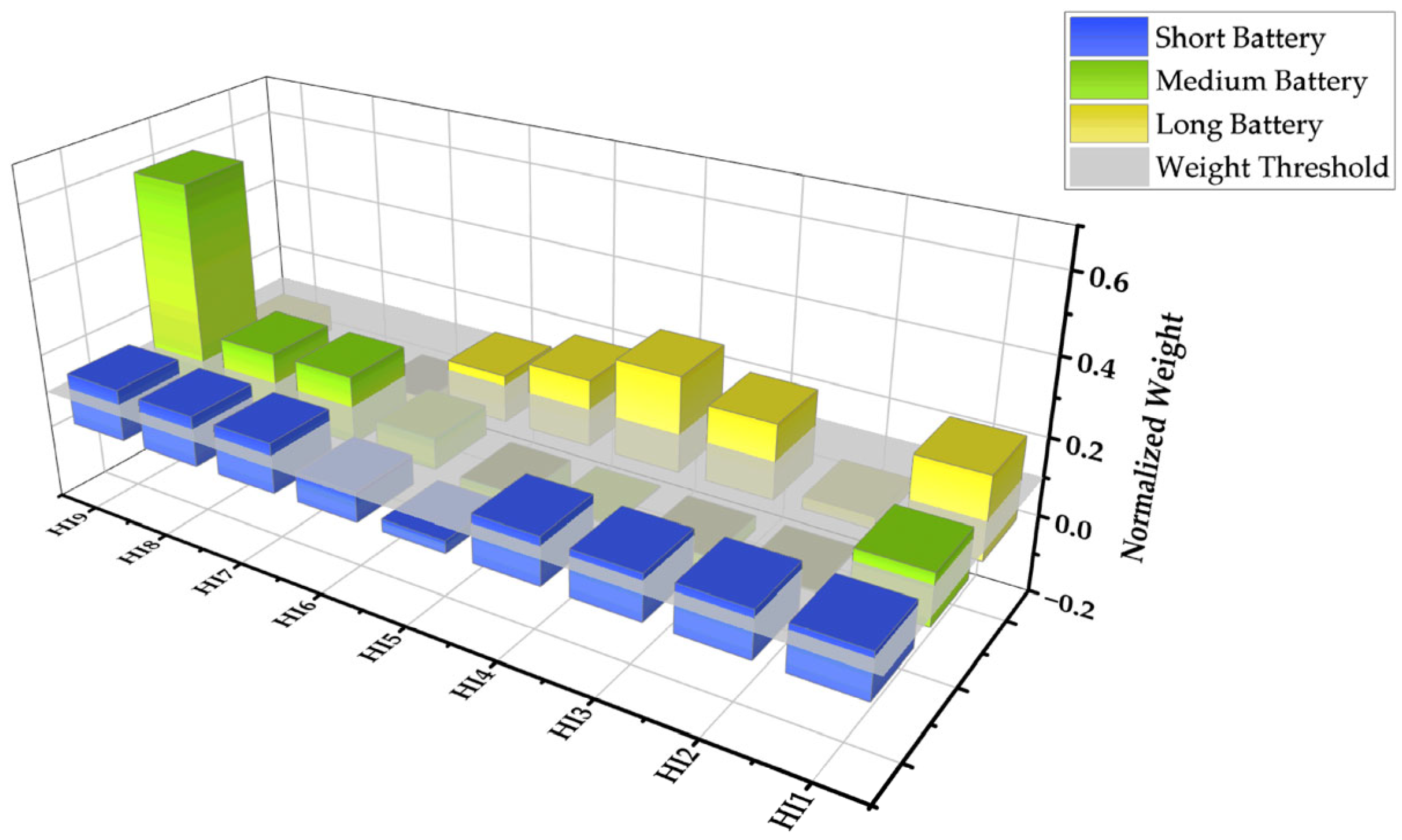
2.2.5. The Correlation Analysis Between Battery Lifetime and HIs

The extracted features are resistant to noise interference. To evaluate the correlation of these nine features with battery cycle life, Spearman correlation analysis [40] is conducted, as defined in Equation (2). The correlation results are presented in

Table 1. Spearman correlation between HIs and battery lifetime.

Notation	Details of Extracted Features	Spearman
HI1	The standard deviation of the difference in discharge capacity curves between Cycle 100 and Cycle 10 versus voltage.	−0.9001
HI2	The peak of the difference in discharge capacity curves between Cycle 100 and Cycle 10 versus voltage.	0.8940
HI3	The difference in discharge capacity in the fixed voltage range (2.6~3.3 V) between Cycle 100 and Cycle 10.	0.8793
HI4	The linear slope of discharge capacity in the fixed voltage range (2.6~3.3 V) with Cycle 2 to Cycle 100.	0.8865
HI5	The difference in the area near the peak voltage of the IC curve (±10%) between Cycle 100 and Cycle 10.	0.8221
HI6	The linear slope of the area near the peak voltage of the IC curve (±10%) with Cycle 2 to Cycle 100.	0.8739
HI7	The mean value of the difference in voltage curves between Cycle 100 and Cycle 10 versus charge capacity (0~0.05 Ah) in 1C CC-CV stage.	−0.8543
HI8	The maximum value of the difference in voltage curves between Cycle 100 and Cycle 10 versus charge capacity (0~0.05 Ah) in 1C CC-CV stage.	−0.8704
HI9	The variance of the difference in voltage curves between Cycle 100 and Cycle 10 versus charge capacity (0~0.05 Ah) in 1C CC-CV stage.	−0.8411

. All absolute values of Spearman correlations of nine features exceed 0.8, indicating a strong association between the extracted HIs and battery cycle life. Therefore, these features can serve both as indicators for identifying degradation patterns and as inputs for battery cycle life prediction models.

$$r=1-{\displaystyle \frac{6{\displaystyle \sum _i^N{d_i}^2}}{N\left(N^2-1\right)}}$$

(2)

where N is the sample size and $d_i$ is the rank difference between the ith feature and the target value.

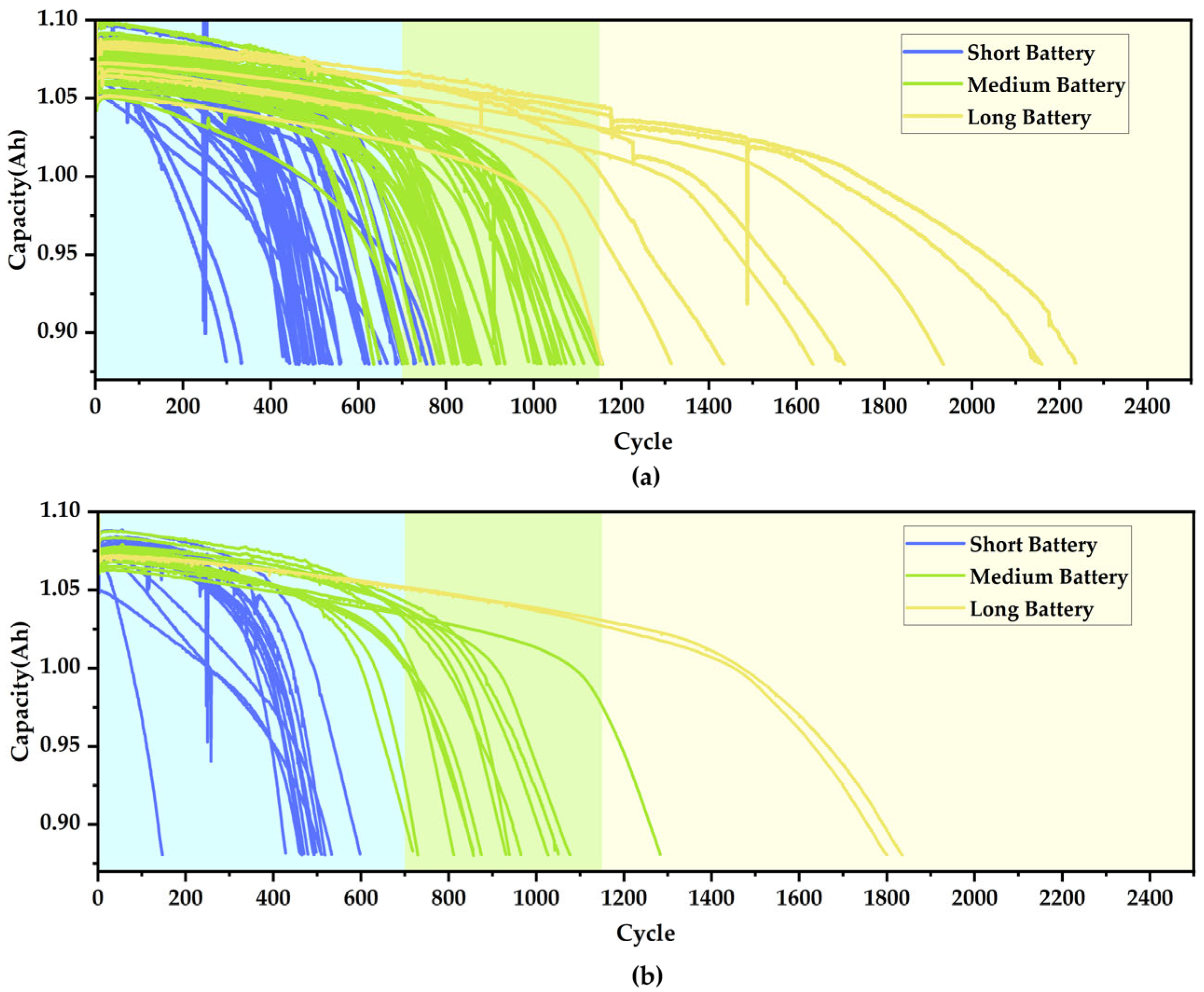
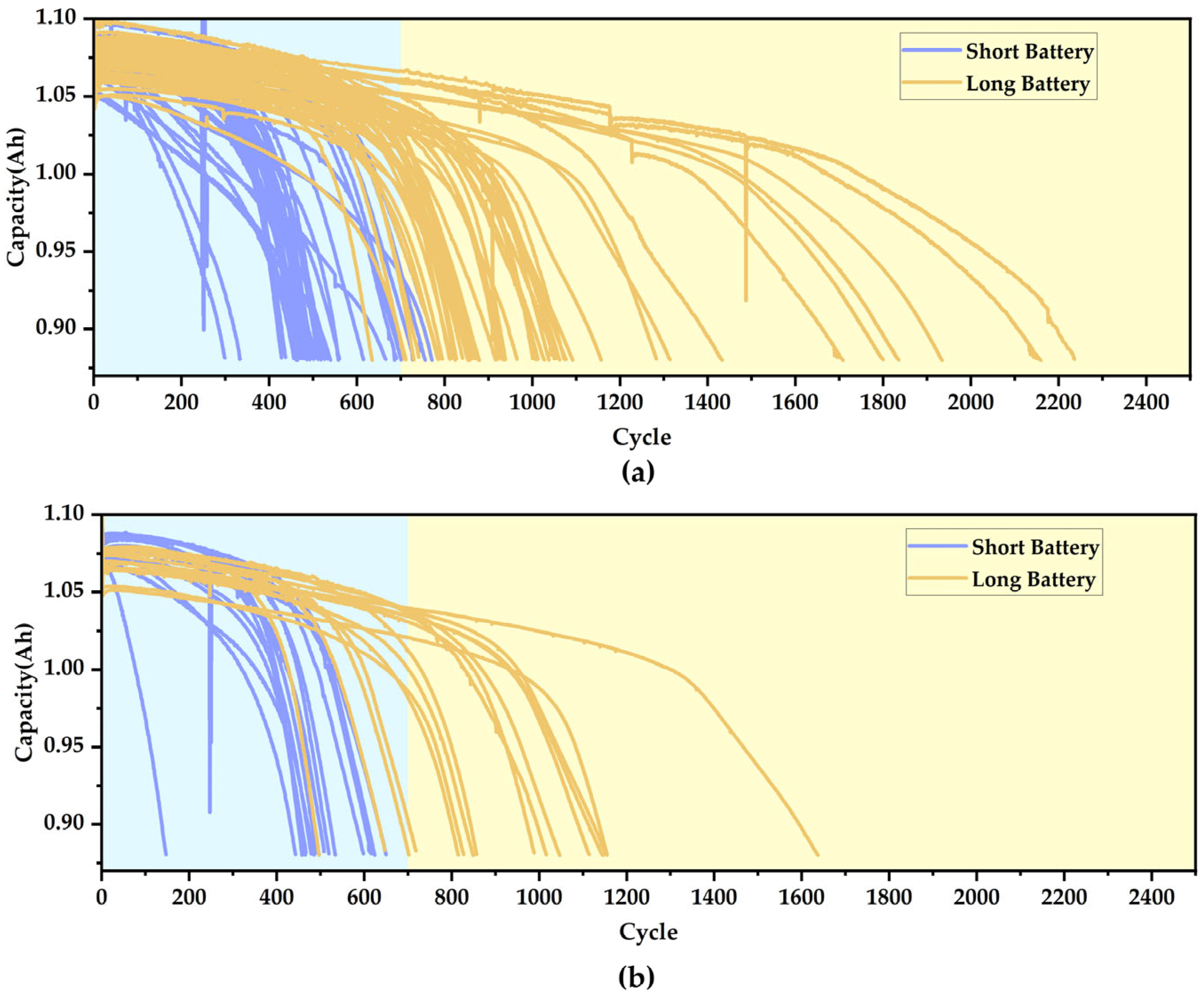
2.3. The Battery Early Degradation Pattern Recognition

Figure 1b demonstrates the different capacity degradation trends of batteries under different fast-charging strategies, with the lifespan showing a huge difference from 148 to 2237 cycles. Batteries with poor aging conditions show a rapid degradation trend, and their lifetimes are relatively short, and vice versa. Batteries with large differences in degradation trends may vary in degradation mechanisms. To make the subsequent life prediction more targeted towards types with similar degradation patterns, the focus of this section is to categorize the aging process into “short battery”, “medium battery”, and “long battery”. To avoid the subjectivity of categorizing them by setting thresholds manually, unsupervised learning classification, i.e., the clustering method, is adopted to categorize the batteries in terms of their degradation patterns.

K-means clustering is one of the most common clustering methods; it divides the samples into clusters according to the distance, as far as minimizing the distance in the cluster and the maximum distance between the clusters [41]. The Euclidean distance is often used, and for an N-dimensional space, the Euclidean distance between two points is shown in Equation (3).

$$d=\sqrt{{\displaystyle \sum _{i=1}^N{\left(x_i-y_i\right)}^2}}$$

(3)

where N denotes the number of dimensions and $x_i$ and $y_i$ are the coordinates of the two points in the ith dimension, respectively.

After unsupervised clustering of cells with unknown degradation patterns, these cells are labeled with a certain pattern. A new cell needs to be classified into a pattern according to its early health features. Therefore, degradation pattern classification is unsupervised clustering, and degradation pattern recognition is supervised classification. The simple K-nearest neighbor (KNN) algorithm is used in this research.

The 9 extracted HIs are processed by natural logarithm to expand their distribution. An approximate ratio of training set: test set = 3:1 is used to determine the number of training sets as 92 and the testing sets as 31, which are randomly chosen. The K-means algorithm is adopted to classify the training set into 3 clusters based on early health features, and the results are shown in Figure 7a. Choosing the number of clusters as 3 will be explained in Section 5.2.1. It is found that the batteries can be roughly grouped according to the fading trends, i.e., “short battery”, “medium battery”, and “long battery”. The KNN algorithm is then used to categorize the testing set into the above 3 patterns, and the results are shown in Figure 7b. It can be seen that the classification algorithm can also recognize the degradation pattern of an unknown battery.

3. Feature Engineering and Supplementary Features Related to Knee

3.1. Feature Engineering

Feature selection is a crucial process in data preprocessing. It focuses on identifying and retaining features that are highly correlated or significant to the target, while eliminating redundant, irrelevant, or low-contribution features. For the three degradation patterns mentioned above, as HIs may contain repetitive information, using all nine HIs directly in modeling may lead to overfitting due to feature redundancy and increase computational burden. Therefore, it is necessary to filter out features that have a greater impact on life prediction for each pattern, which is what feature engineering aims to achieve.

Traditional feature engineering approaches are categorized into three methods: filtering, wrapping, and embedding. The filtering method evaluates individual features based on their dispersion or relevance to the target, and then selects features by establishing a threshold or specifying the number of features to retain. The wrapping methods iteratively select or exclude certain features, assessing each subset using an objective function to identify the optimal feature combination. The embedding method involves training a model to obtain feature weight coefficients, and then selecting features according to these coefficients. However, traditional filtering methods typically only assess the correlation between individual features and the target, instead of accounting for feature interactions. Wrapping methods often incur high computational costs due to the complicated training process. Additionally, the weight coefficients obtained from the embedding method usually lack clear interpretability and are less effective in handling feature redundancy. Consequently, this research employs the more interpretable and efficient Relief algorithm to address these limitations.

The Relief algorithm, first introduced by Kira [42], assesses the correlation between features and classes based on a feature’s ability to distinguish between nearby samples. When a feature shows large differences between instances with significant prediction disparities, its weight increases, indicating strong prediction power. Conversely, if a feature has substantial differences between instances with minor prediction disparities, its weight decreases, suggesting weak prediction ability, which needs to be removed [43]. The core of the Relief algorithm lies in updating feature weights. Let P (diff A) be the probability that the selected instances have a different feature A, and P (diff C) be the probability that the selected instances have different predictions. Based on conditional probability, P (diff C|diff A) represents the probability that the selected instances have different predictions given that their feature A varies. According to Bayes’ rule, the updated weight of feature A is shown in Equation (4). Notably, the Relief algorithm and its variants represent the sole standalone evaluation filter methods capable of identifying feature dependencies. These algorithms utilize nearest-neighbor principles to compute feature statistics that indirectly capture interactions, while preserving the inherent advantages of filter approaches, such as computational efficiency.

$$Weight\left[A\right]={\displaystyle \frac{P\left(\mathit{diff} C|\mathit{diff} A\right)\cdot P\left(\mathit{diff} A\right)}{P\left(\mathit{diff} C\right)}}-{\displaystyle \frac{\left[1-P\left(\mathit{diff} C|\mathit{diff} A\right)\right]\cdot P\left(\mathit{diff} A\right)}{1-P\left(\mathit{diff} C\right)}}$$

(4)

In this study, the Relief algorithm is applied to the feature engineering of three battery degradation patterns, i.e., “short battery”, “medium battery”, and “long battery”. The normalized weights of each HI are presented in Figure 8. A weight threshold of 0.1 is used to eliminate redundant or negative features. After the feature engineering process, seven, four, and five valid features are retained for the subsequent life prediction, respectively. The Relief function introduced in MATLAB R2010b is used.

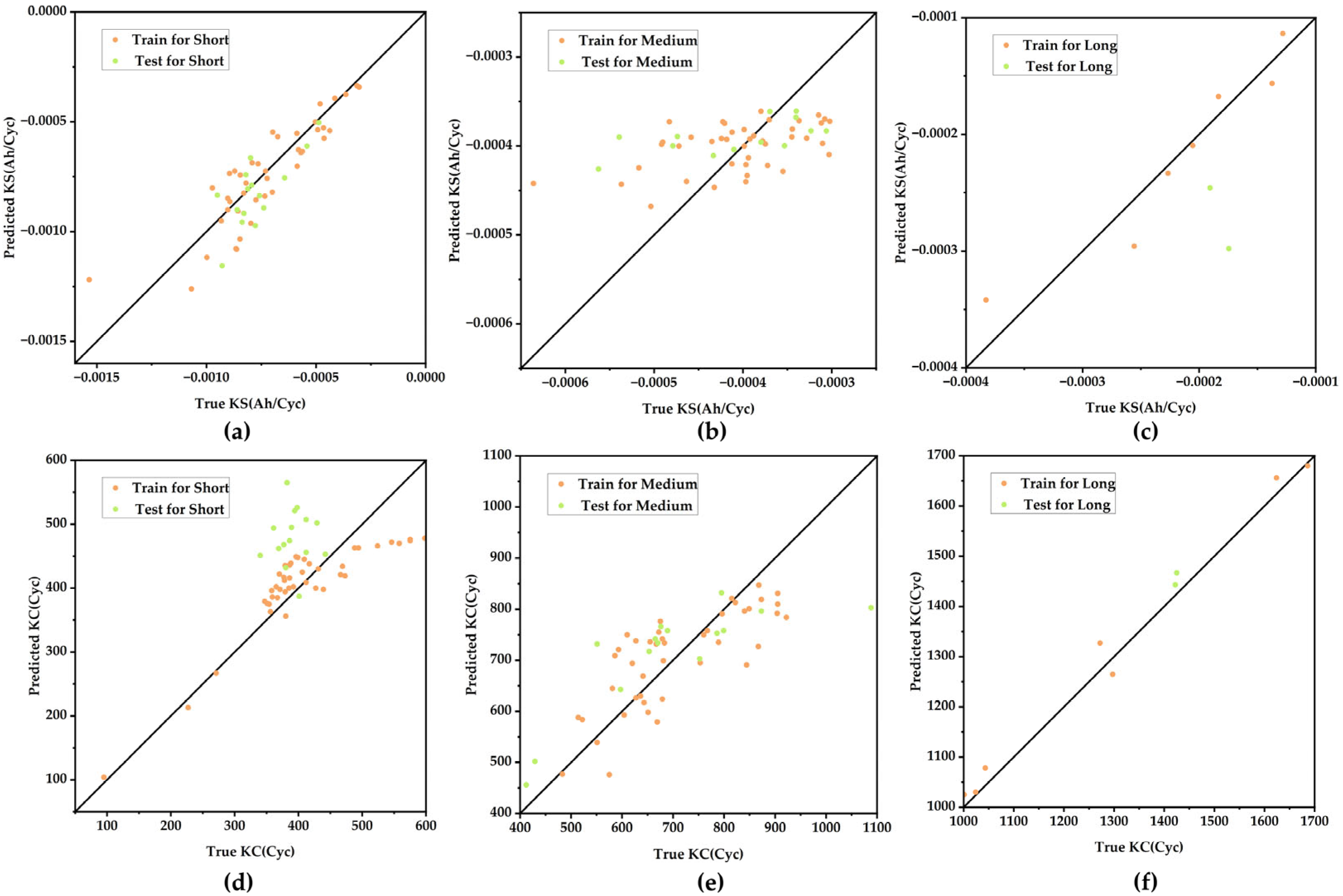
3.2. Identification of Supplementary Features Related to Knee Point

A notable challenge in lithium-ion battery life prediction is the nonlinear performance degradation after long-term cycling. This not only shortens the battery’s lifetime, but also affects its safety and becomes a technological bottleneck that hinders its reliable application. Most of the current data-driven lifetime or SOH prediction uses direct or indirect external characteristics such as temperature, voltage, current, and capacity as HIs. As the onset of nonlinear degradation, the knee point contains vital aging information that may provide additional information for accurate RUL estimation. This enables more proactive measures to prolong battery life and facilitate the determination of the ideal battery retirement time [44].

It has been demonstrated that the knee point signifies the onset of a rapid capacity degradation trend leading to EOL [45,46]. Numerous studies have demonstrated that an accelerated nonlinear aging phase emerges from a particular stage of the battery aging process. He et al. [47] performed multiple charge/discharge tests on lithium cobalt oxide/graphite batteries at room temperature and observed that the capacity fade occurs in a nearly linear fashion, followed by a pronounced reduction. Yang et al. [48] also found that NCM battery capacity decays slowly in hundreds of cycles before the knee point, while the degradation rate becomes relatively sharp after that point; this can be described by a two-term logarithmic model. In actuality, knee points occur under all operating conditions and can appear before or after the EOL is reached [6]. The “knee” of the capacity fade is also mentioned in the IEEE Standard 485™-2010 “IEEE Recommended Practice for Sizing Lead-Acid Batteries for Stationary Applications” [49] to guide battery replacement.

Meanwhile, several methods have also been designed to identify the battery’s knee point offline. Establishing a standardized definition and methodology for identifying the knee point can enhance battery prediction systems, particularly in RUL modeling, fostering more accurate and reliable battery management and performance optimization. Satopaa et al. [50] identified the knee point by selecting the point of maximum curvature on the curve, which corresponds to where the curvature direction changes—namely, the transition between concave and convex shapes. Diao et al. [6] uniquely defined the knee point as the cycle number at the intersection of two tangents on the capacity decay curve, which can be obtained from the points with the minimum and maximum absolute slope-changing ratio. Fermín-Cueto et al. [51] innovatively proposed the concept of the “knee-onset” based on the above double tangent method to define the point at which the battery shows the first signs of the transition to the accelerated degradation phase. The knee point is defined by Zhang et al. [52] as the intersection of two straight lines with distinct slopes, which precisely characterizes the two stages of capacity degradation. However, employing gradients to determine these slopes proves to be unreliable, due to the noise in experimental data. Bacon and Watts’ model [53] offers a robust method for identifying knee points without relying on the gradient approach. This model, as presented in Equation (5), expresses the relationship between two straight lines near a transition point x₁.

$$y={\alpha }_0+{\alpha }_1(x-x_1)+{\alpha }_2(x-x_1)\tanh \left\{(x-x_1)/\gamma \right\}+z$$

(5)

where ${\alpha }_0$ represents the intercept at the knee point x₁; ${\alpha }_1$ and ${\alpha }_2$ denote, respectively, the slopes of the two-stage degradation; $\gamma$ is the degree of abruption at the intersection of the two straight lines at $x_1$; and $z$ is a random variable accounting for error.

Figure 9 shows the knee points identified by the Bacon–Watt two-stage model. Taking the 123rd cell as an example, the red line shows the two stages of decline, and the location of the knee point is identified by the intersection point. We can also see that the majority of batteries in this accelerated aging dataset follow a two-stage degradation, with a capacity dive starting at around 1 Ah, i.e., 90% SOH, and then quickly reaching EOL. In general, the longer the lifetime the batteries have, the later the knee point arrives. For this accelerated decline dataset where the knee point precedes the EOL point, it can provide additional information for the lifetime prediction. We found that the Spearman coefficients between the four features of fast decline slope, slow decline slope, knee point cycle, knee capacity, and the battery life are, respectively, 0.8174, 0.9214, 0.9877, and −0.0222. Using the features extracted in the early stage to predict the rate of fast capacity decline, and further to predict the RUL may not be reliable. And the knee capacity, as shown in Figure 9, mostly occurs near 90% SOH, which is not significant for life prediction. After analysis, we extract the knee slope of the slow decline phase (KS) and the knee cycle (KC) as additional features for subsequent battery life prediction. Figure 10 shows the variation of KS and KC with battery lifetime. It can be seen that the KS and KC features are strongly correlated with the lifetime, and as they are not features that can be computed from physical measurements, they can only be obtained by predictive methods.

4. RUL Prediction Method

This section details the methodologies employed in the proposed RUL prediction approach. A data-driven approach for battery early cycle life prediction based on PSO-GPR is proposed. Notably, battery lifetime prediction models are developed separately for each of the 3 degradation patterns.

4.1. GPR-Based Prediction Model

In the proposed capacity estimation approach, a data-driven technique is utilized. GPR serves as a robust regression method, exhibiting strong adaptability in addressing nonlinear issues [54] and performing effectively in battery state estimation and health diagnosis [55]. Furthermore, the GPR model holds significant potential for achieving accurate estimation even for fewer samples for modeling [54,56].

A Gaussian process (GP) is a stochastic process defined over a continuous domain, wherein each point in the input space corresponds to a normally distributed random variable [57]. In addition, each finite set of these random variables complies with a multidimensional normal distribution. The distribution of a Gaussian process is characterized as the joint distribution of infinitely many random variables. Therefore, it constitutes a functional distribution over a continuous domain. A Gaussian process is uniquely defined by a mean function and a kernel function, which can be represented as Equation (6).

$$f\left(x\right)~GP\left(m\left(x\right),k_f\left(x,x’\right)\right)$$

(6)

where $m\left(x\right)$ is the mean function and $k_f\left(x,x’\right)$ is the kernel function.

Gaussian process regression (GPR) is a nonparametric modeling approach grounded in Bayesian theory, capable of handling uncertain output variables. The fundamental concept of GPR involves treating a stochastic process composed of multiple random variables as a high-dimensional joint Gaussian distribution [57], as well as to construct a nonparametric model for regression analysis with the Gaussian process prior, i.e., the process of deriving the posterior from the prior and the observations.

A Gaussian process is uniquely defined by a mean function and a kernel function, which is called a prior. After obtaining a set of observations (i.e., the training set), the mean and kernel functions of this Gaussian process can be modified based on the observations and then used to predict the posterior values (i.e., the testing set). Assuming that S is the training set, which is independently and identically distributed, a Gaussian process regression model is defined as shown in Equation (7).

$$y=f\left(x\right)+\epsilon$$

(7)

where y is an observation and $\epsilon$ is an independent and identically distributed noise variable that obeys $\epsilon \sim N\left(0,{{\sigma }_n}^2\right)$.

Thus, the prior distribution of observations is represented in Equation (8).

$$y\sim N\left(m\left(x\right),K_f\left(x,x\right)+{{\sigma }_n}^2{I}_n\right)$$

(8)

where $I_n$ is an n-dimensional unit matrix, ${{\sigma }_n}^2{I}_n$ is the noise covariance matrix, and $K_f\left(x,x\right)$ is a symmetric positive definite matrix with the following Equation (9).

$$K_f\left(x,x\right)={\left(k_f\left(x^i,x^j\right)\right)}_{n\times n}$$

(9)

The main purpose of training a GPR model is to obtain the parameters $\theta$ of the mean and kernel functions. Given the parameters, the optimization aims to maximize the probability of the training set observations. To achieve this, a conjugate gradient descent method is employed to minimize the negative log marginal likelihood (NLML), which is shown in Equation (10).

$$NLML=-\log P\left(y|x,\theta \right)={\displaystyle \frac{1}{2}}{y}^T{\left[K_f\left(x,x\right)+{{\sigma }_n}^2{I}_n\right]}^{-1}y+{\displaystyle \frac{1}{2}}\log \left(\det \left(K_f\left(x,x\right)+{{\sigma }_n}^2{I}_n\right)\right)+{\displaystyle \frac{n}{2}}\log 2\pi$$

(10)

After determining the kernel function parameters, a Gaussian process regression (GPR) model was developed and subsequently employed to predict the testing set using the posterior distribution. As a stochastic process, GP assumes that new input data (i.e., the inputs of the testing set) follow the Gaussian distribution of the training set. Consequently, the joint prior distribution of the observed value y and the predicted value y* at the prediction point x* is presented in Equation (11).

$$\left(\begin{array}{c}y\\ y*\end{array}\right)\sim N\left(\left(\begin{array}{c}m\left(x\right)\\ m\left(x*\right)\end{array}\right),\left[\begin{array}{cc}{K}_f\left(x,x\right)+{{\sigma }_n}^2{I}_n& K_f\left(x,x*\right)\\ K_f{\left(x,x*\right)}^T& K_f\left(x*,x*\right)\end{array}\right]\right)$$

(11)

According to the properties of the multivariate Gaussian distribution, it can be shown in Equation (12) that y* satisfies the multivariate Gaussian distribution.

$$y*|x,y,x*\sim N\left(m*,\Sigma *\right)$$

(12)

$$m*=K_f\left(x,x*\right)\left[{\left(K_f\left(x,x\right)+{{\sigma }_n}^2{I}_n\right)}^{-1}\left(y-m\left(x\right)\right)\right]+m\left(x*\right)$$

(13)

$$\Sigma *=K_f\left(x*,x*\right)-K_f{\left(x,x*\right)}^T{\left[K_f\left(x,x\right)+{{\sigma }_n}^2{I}_n\right]}^{-1}{K}_f\left(x,x*\right)$$

(14)

where the mean m* is taken as the predicted value of the testing set and the covariance predicted value Σ* reflects the uncertainty of the GPR model.

A diagram of the GPR algorithm is shown in Figure 11. This figure illustrates how GPR predicts the underlying function based on sparse observations, providing both the mean prediction and its associated uncertainty—showing higher confidence near observed data and increasing uncertainty in regions without observations.

The kernel function is the core of the Gaussian process, which serves as a measure of the “distance” between two points in GP.

Table 2. Common one-dimensional kernel functions.

Kernel	Formula	Parameter
Squared Exponential	$k_{SEiso}\left(x,x’\right)={s_f}^2\exp \left(-{\displaystyle \frac{{‖x-x’‖}^2}{2l^2}}\right)$	${s_f}^2,l$
Matérn	$k_{Matern}\left(x,x’\right)={s_f}^2{\displaystyle \frac{2^{1-v}}{\Gamma \left(v\right)}}{\left({\displaystyle \frac{\sqrt{2v}‖x-x’‖}{l}}\right)}^v{K}_v\left({\displaystyle \frac{\sqrt{2v}‖x-x’‖}{l}}\right)$	${s_f}^2,v,l$
Exponential	$k_{Exponential}\left(x,x’\right)={s_f}^2\exp \left(-{\displaystyle \frac{‖x-x’‖}{l}}\right)$	${s_f}^2,l$
γ-Exponential	$k_{\gamma }\left(x,x’\right)={s_f}^2\exp \left(-{\left({\displaystyle \frac{‖x-x’‖}{l}}\right)}^{\gamma }\right)$	${s_f}^2,l,\gamma$
Rational Quadratic	$k_{RQ}\left(x,x’\right)={s_f}^2{\left(1+{\displaystyle \frac{{‖x-x’‖}^2}{2\alpha l^2}}\right)}^{-\alpha }$	${s_f}^2,l,\alpha$
Polynomial	$k_{Polynomial}\left(x,x’\right)={s_f}^2{\left(ax\cdot x’+c\right)}^d$	${s_f}^2,a,c,d$

lists common single kernel functions [58]. Parameters within these functions, such as ${s_f}^2$, l, v, $\gamma$, $\alpha$, a, c, and d, are kernel parameters.

The mean function is generally selected to be zero mean. Commonly used kernel functions include squared exponential kernels, Matérn kernels, and polynomial kernels. Considering the overall degradation trend and local regeneration phenomenon of battery aging, a single kernel function may not capture the different trends well, so the complex problem can be described by combining different single kernel functions to construct a composite kernel function, which can combine the advantages of different kernel functions to better accommodate different types of data. Composite kernel functions are obtained by addition or multiplication operations on the single kernel functions, because they are closed in these operations. In this study, additive operations are applied to squared exponential (SEiso) and Matérn (Matérniso) kernels [59] based on an isotropic length-scale Gaussian distribution. The smoothing coefficient of the Matérniso kernel is taken as 3 (indicating moderate smoothing). The equations for the single and composite kernels are shown below.

$$k_{Materniso}\left(x,x’\right)={s_f}^2\left(1+{\displaystyle \frac{\sqrt{3}}{l}}‖x-x’‖\right)\exp \left(-{\displaystyle \frac{\sqrt{3}}{l}}‖x-x’‖\right)$$

(15)

$$k_{SEiso+Materniso}\left(x,x’\right)=k_{SEiso}\left(x,x’\right)+k_{Materniso}\left(x,x’\right)$$

(16)

where ${s_f}^2$ and l control, respectively, longitudinal and transverse extensibility, whose initial values are hyperparameters that PSO needs to identify.

GPR can not only provide a single-point estimation of battery life; it can also give a confidence interval for the results, which can give more reliable information for the battery management system (BMS) by evaluating the uncertainty of the prediction result. This probabilistic output allows the BMS to make risk-aware decisions, especially under noisy measurements or limited data. Compared to other models like neural networks or SVMs, which provide only deterministic predictions, GPR naturally handles nonlinearity, performs well with small datasets, and avoids overfitting through its Bayesian framework. These advantages make it particularly suitable for real-world battery prognostics where data quality and quantity may be limited. The Gaussian processes for machine learning (GPML) toolbox is used in this study [60]. The version 4.1 dated 19 October 2017 of the GPML MATLAB code package is used.

4.2. PSO-Based Hyperparameter Optimization

The initial values of a set of parameters, called hyperparameters [61], need to be given in advance in the prior process, and their accuracy affects the effectiveness of model training. Aiming at the problem that it is difficult to converge to a better result in a short time in the conventional hyperparameter tuning algorithm, the particle swarm optimization is adopted. Hyperparameter optimization methods like grid and random search are often inefficient or unreliable, while PSO offers a robust, fast-converging, and easy-to-implement solution particularly suited for tuning models on small to medium-sized battery degradation datasets in this research [62].

Inspired by the foraging behavior of birds, Kennedy and Eberhart introduced the PSO algorithm in 1995 [62]. It is highly regarded for its rapid convergence, minimal parameter requirements, and simplicity. These qualities make it a popular choice across various domains such as function optimization, neural network training, data mining, and fuzzy systems [63]. A flock of birds searches for the biggest food in the whole forest. All the birds share the location and size of the food they found each time, and adjust the search direction in the next search. Similarly, the optimal hyperparameters can be found iteratively in the parameter space. The realization of PSO depends on the social sharing of information. The general flow of the PSO algorithm is shown in Figure 12.

The velocities and positions are updated in each iteration as the following Equations (17) and (18).

$$v_i^{k+1}=w·v_i^k+c_1{r}_1\left(pbes{t}_i^k-x_i^k\right)+c_2{r}_2\left(gbes{t}^k-x_i^k\right)$$

(17)

$$x_i^{k+1}=x_i^k+v_i^{k+1}$$

(18)

where $v_i^k$, $x_i^k$, and $pbes{t}_i^k$ are, respectively, the velocity, position vector, and historical optimal position of the ith particle at the kth iteration; w is the inertial weighting; $c_1$ and $c_2$ are the self-learning factor and group-learning factor, which represent the ability of particles to learn from the historical record of itself as well as the group; $r_1$ and $r_2$ are random numbers between 0 and 1; and $gbes{t}^k$ is group optimal position at the kth iteration.

The above represents that the direction of movement of each particle for the next iteration equals the inertia direction plus the individual optimal direction plus the group optimal direction. Therefore, each time it takes a random point is not “purposelessly” taken, but taken in the direction of improving the model.

4.3. The General Framework of the RUL Prediction Method

The general framework of the proposed RUL prediction method is shown in Figure 13. Firstly, 9 HIs highly correlated with cycle life are extracted from the batteries’ first 100 cycles of charge/discharge data. Moreover, the batteries are recognized into 3 different degradation patterns based on the extracted 9 HIs. Additionally, the Relief algorithm is used to eliminate low contribution features in 3 patterns, reducing the HIs to 7, 4, and 5, respectively. Then, 3 life prediction models based on GPR are established, whose hyperparameters are tuned using PSO. In the first step, the KS and KC are predicted, respectively, using the secondary extracted features. After that, the predicted KS and KC are used as complementary features along with the regular HIs for predicting the battery lifetime. Finally, the performance of the model is evaluated with the mean absolute percentage error.

To assess the accuracy of the battery life prediction results, the mean absolute percentage error (MAPE) is used as per the following Equation (19). The MAPE does not change according to the global scaling of the target variable, making it suitable for battery life, which has a wide distribution in this study.

$$\mathrm{MAPE}={\displaystyle \frac{100\%}{n}}{\displaystyle \sum _{i=1}^n\left|\frac{{\widehat{y}}_i-y_i}{y_i}\right|}$$

(19)

where ${\widehat{y}}_i$ and $y_i$ are, respectively, the prediction and the actual values of battery cycle life.

5. Results and Discussion

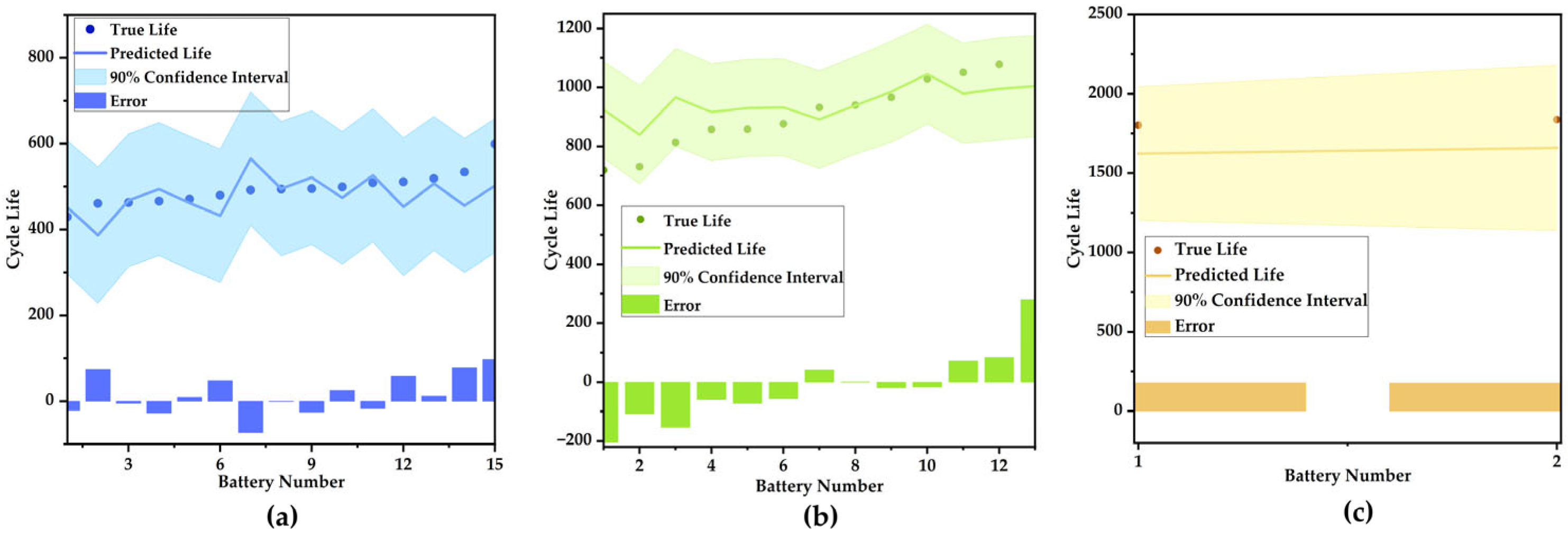
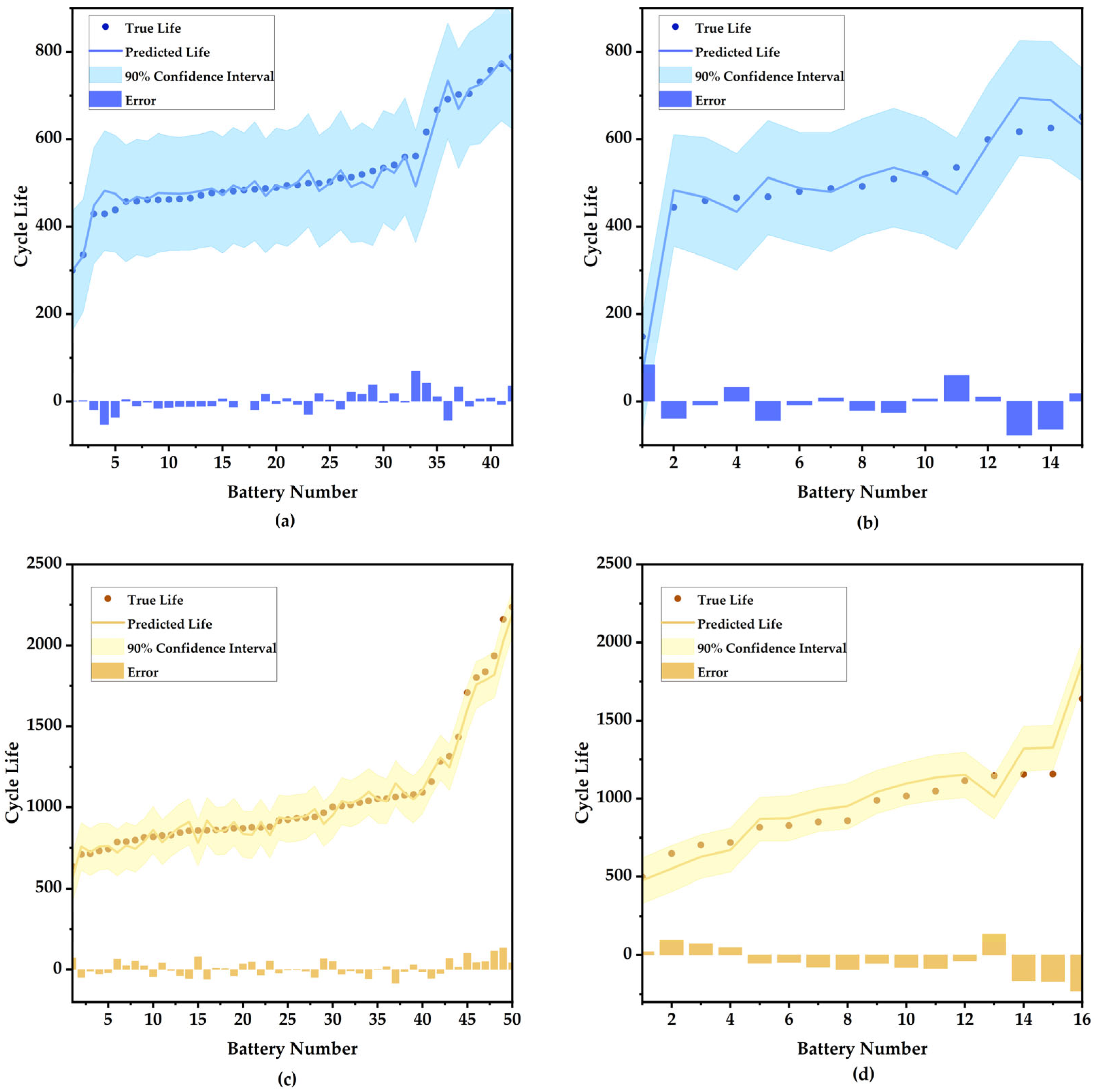
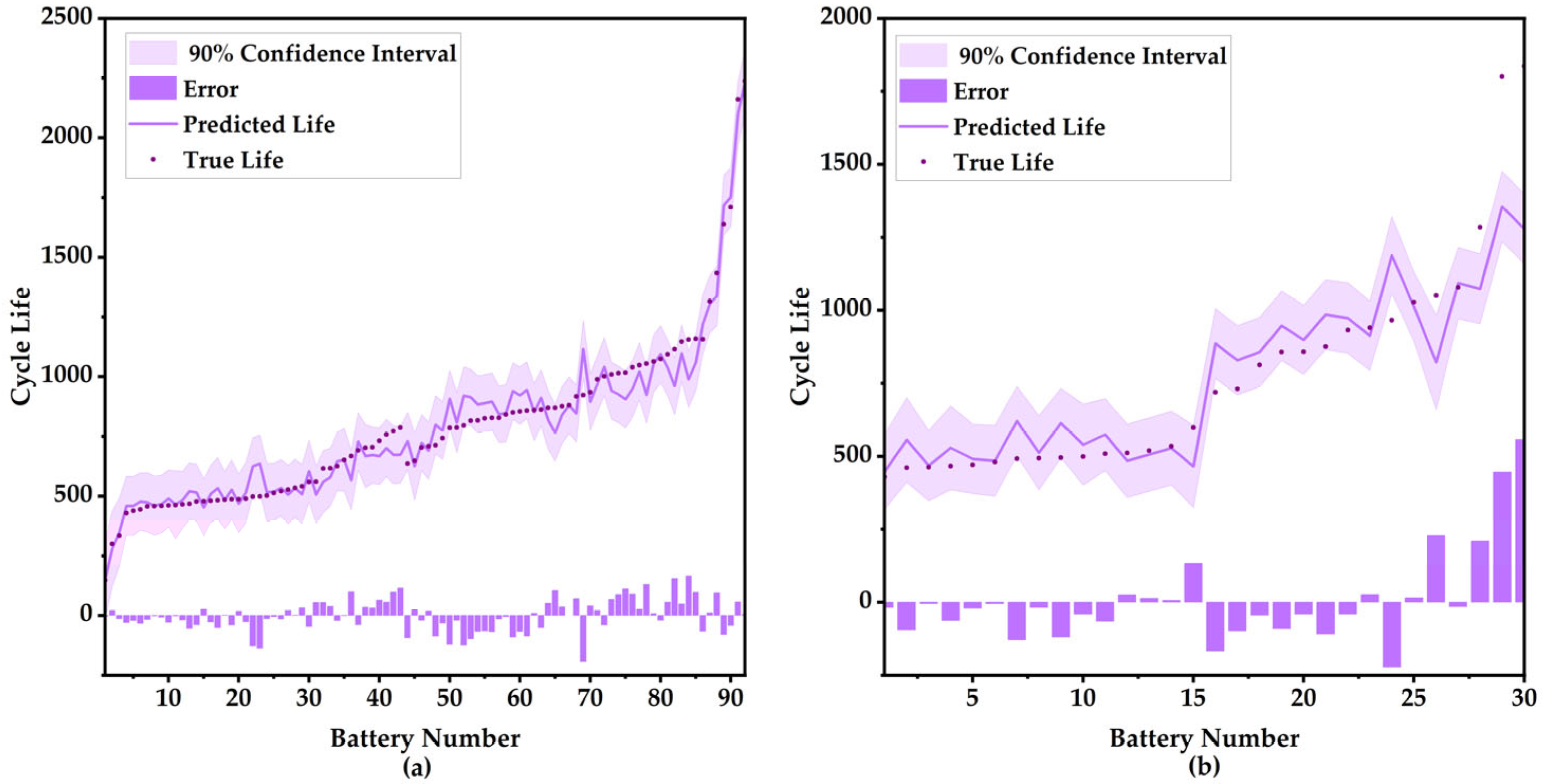
5.1. The Verification of RUL Prediction

Three life prediction models based on GPR were established. Using the optimized initial values of the kernel function parameters, the prediction models of KS and KC were first constructed, and the prediction results are shown in Figure 14. It can be seen that the predicted KS and KC for the training and testing sets are scattered around the true values. The predicted KS and KC were utilized as supplementary features to further build the prediction model of RUL, and the prediction results are shown in Figure 15. In addition to the predicted means, 90% confidence intervals are also given.

It can be found that the MAPEs for training and testing sets are 7.08% and 7.55% (for short batteries), 8.96% and 9.87% (for medium batteries), and 1.91% and 9.76% (for long batteries). The quantitative results indicate that the proposed method attains a high prediction accuracy, with an overall mean absolute percentage error (MAPE) of approximately 8.70%. The MAPE of medium batteries is the biggest among all. This may be due to the fact that the selected HIs are more dispersed at both shorter and longer lifetimes. Consequently, these features differ more between batteries with different lifetimes, resulting in stronger lifetime characterization. In contrast, the intermediate region exhibits a more centralized distribution. Here, the differences in health features among batteries with different lifetimes are smaller, leading to relatively weaker lifetime characterization. The majority of prediction values lie in 90% uncertain intervals, which demonstrates the validity of the prediction. The widening of the 90% confidence intervals for the testing sets of three degradation patterns suggests that the predictions are becoming less reliable. This also confirms the basic concept of early life prediction, i.e., when using only the features extracted from the first 100 cycles, the longer the batteries live, the lower the reliability of the prediction is.

As the onset of nonlinear degradation, the knee point contains vital aging information about when nonlinear aging begins to occur, which provides additional information for accurate RUL estimation. Traditional lifetime prediction algorithms predict SOH or RUL based on direct or indirect HIs. MAPE is, respectively, 10.29% (short batteries), 10.62% (medium batteries), and 16.44% (long batteries) without supplementary features related to the knee. Although there exist errors in predicting KS and KC based on HIs, which may introduce cumulative errors into the RUL predictions, the aging-related information provided constitutes a more significant share than errors.

5.2. The Comparison with Other Models

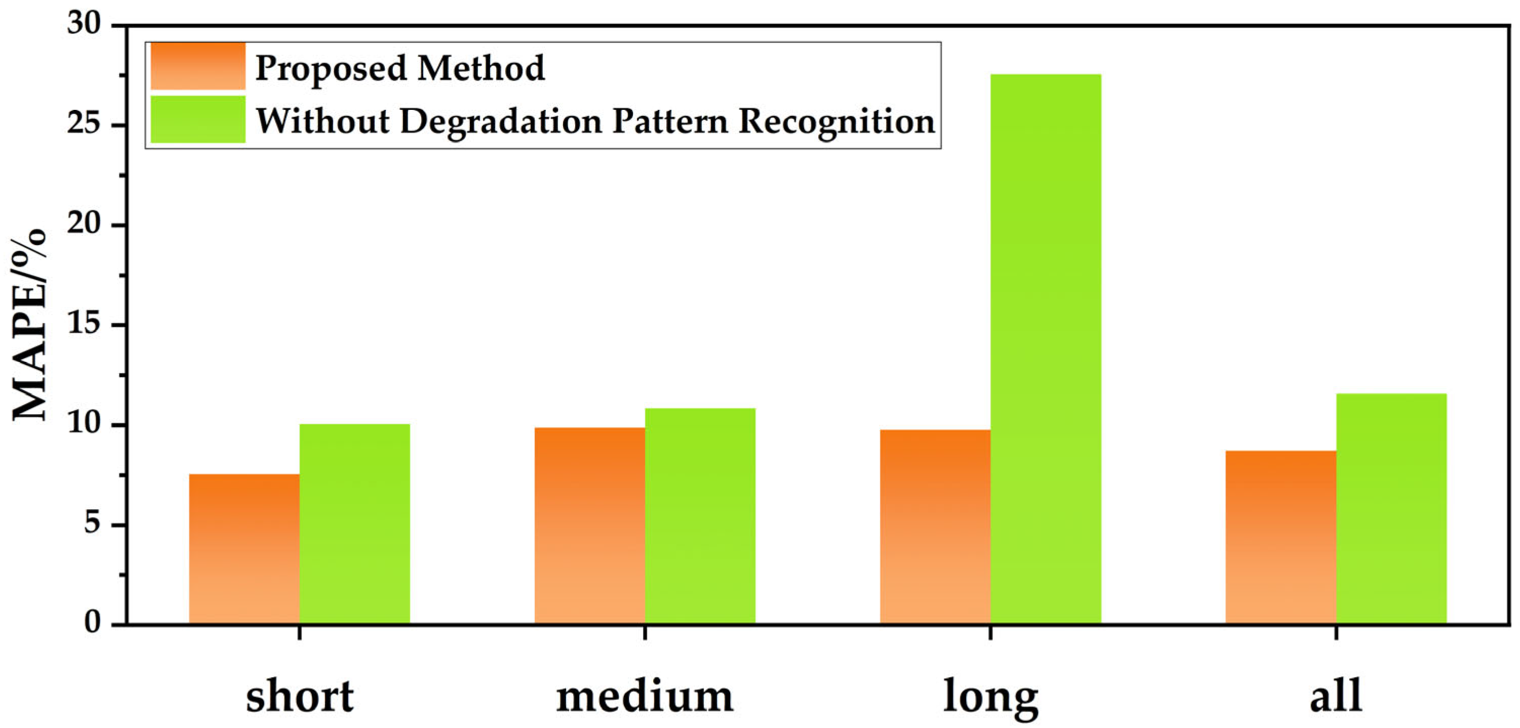
5.2.1. Validation Result with Different Cluster Number

In Section 2.3, we divided the batteries into three degradation patterns, because the early aging of batteries in different life intervals may behave differently. To make the life prediction more targeted towards similar types, degradation pattern recognition was considered in advance. This prevents short-life batteries from being influenced by long-life batteries. In actuality, three is an artificially formulated number of clusters, i.e., short batteries, medium batteries, and long batteries. Suppose the number of clusters is set even lower, e.g., only two types of batteries are classified, i.e., short batteries and long batteries, as presented in Figure 16. We can see that the extracted HIs also achieve better classification results. A similar approach was used for feature engineering, as well as for PSO-GPR modeling in two degradation patterns separately. The prediction results are shown in Figure 17. The MAPE for training and testing sets are 3.20% and 9.05% (for short batteries) and 3.93% and 9.29% (for long batteries). The MAPE for all testing batteries is 9.17%.

Similarly, for the model with the cluster number of one, i.e., without degradation pattern recognition, the prediction results are shown in Figure 18. The MAPEs for the training and testing sets are 6.72% and 11.56%.

Figure 19 performs the comparison between the proposed method and the traditional method without degradation pattern recognition (i.e., one cluster). It can be seen that in three clusters, the proposed method outperforms the traditional one, which indicates the effectiveness of degradation pattern recognition.

For this dataset with a fixed total number of batteries, as the number of clusters decreases, the number of training batteries in each cluster increases, which is more favorable for the machine learning model, but also brings the problem of a large span of battery lifetimes in the same pattern, and a large aging mechanism difference exists in the mutual influence. In addition, when comparing Figure 15, Figure 17 and Figure 18, it is found that the larger the size of the training set, the narrower the 90% confidence interval of the testing set, which indicates that the credibility of the prediction is higher. But for long batteries with a small number of the training set, the credibility of the prediction is not high. This is also in line with the cognitive law. Therefore, we need to decide how to divide the degradation patterns according to the size of the available training dataset and ensure that the number of batteries in each type is as uniform as possible.

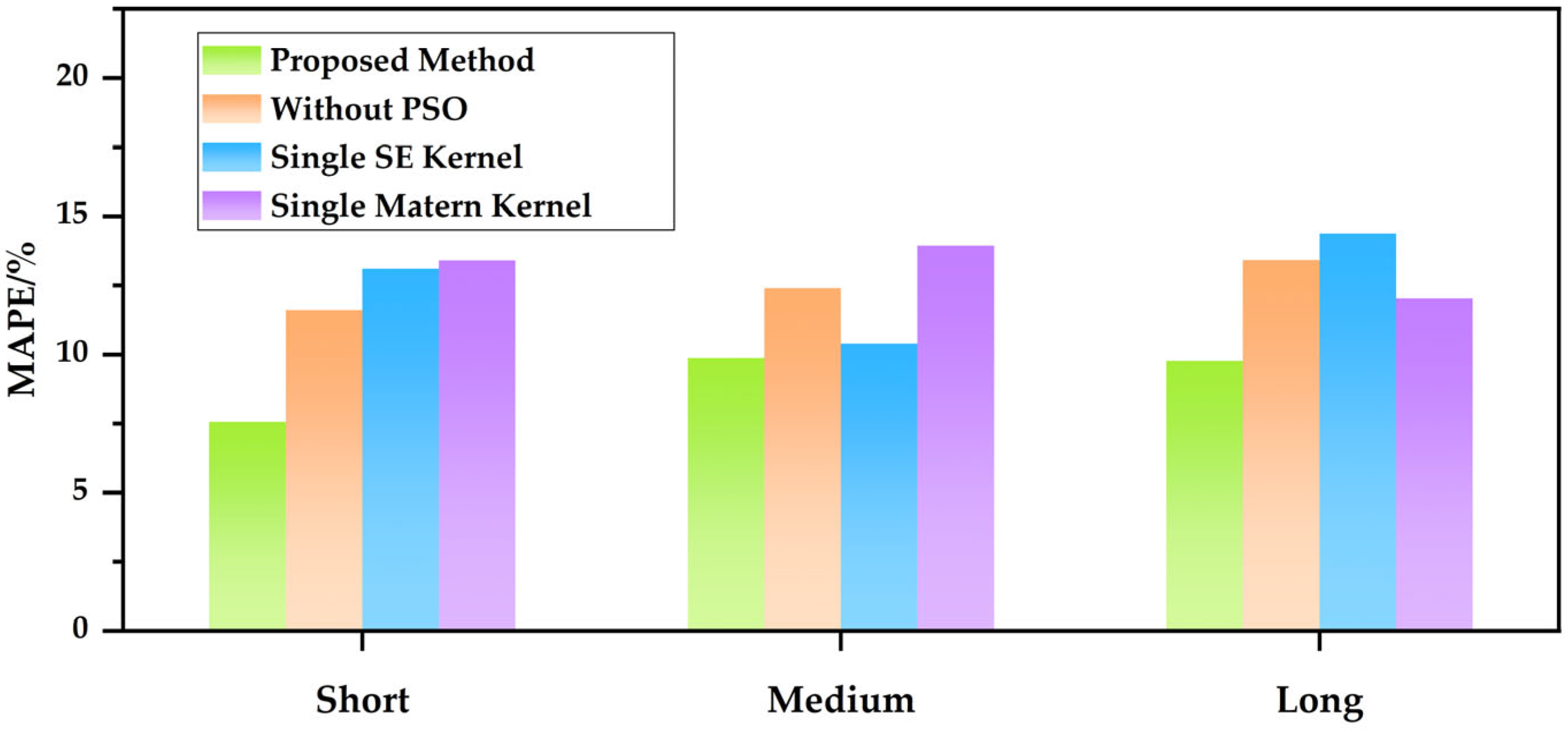
5.2.2. Validation Result with Different GPR Kernels

A Gaussian process is uniquely defined by a mean function and a kernel function. The kernel function is the core of the Gaussian process. We combined squared exponential and Matérn kernels to construct a composite kernel function in this study, whose hyperparameters were tuned based on the PSO algorithm. To verify the superiority of the proposed method, Figure 20 shows the comparison between the proposed method and two traditional methods, including GPR without hyperparameter optimization (s_f = 2 and l = 0.9) and GPR with single kernel functions (squared exponential kernel and Matérn kernel). The comparison reveals that the proposed battery life prediction in this work outperforms the other two models; we can achieve an early and roughly accurate single-point prediction of battery life.

The main purpose of training a GPR model is to obtain the parameters of GP, and then make a posterior prediction. The initial values of the parameters are those that need to be set manually before machine learning, rather than those obtained by the model through training, and their accuracy affects the effectiveness and efficiency of model learning. Manual tuning requires expert experience, which is cumbersome and time-consuming for models with a large number of hyperparameters as in this study. Therefore, it makes sense to adopt this purposeful search-tuning algorithm.

Composite kernels, formed by combining basic kernels through addition and multiplication, can capture a wider range of data structures. This flexibility allows them to adapt to diverse data patterns more effectively than single kernels, which are limited to specific structures like local variations or periodicity. Additionally, composite kernels decompose complex data into interpretable components. For instance, in time series analysis like the Mauna Loa atmospheric CO₂ dataset [64], they can break down data into long-term trends, annual periodicity, and short-term deviations, facilitating human understanding and model validation. Therefore, composite kernel functions have advantages over single kernel functions in this research.

5.2.3. Validation Result with Other Algorithms

To further assess the performance of the proposed early battery life prediction method, this section presents a comparative analysis against various alternative algorithms. Five common machine learning algorithms are utilized, including back propagation (BP), SVM, random forest (RF), CNN, and LSTM. As mentioned in

Table 3. The comparison between PSO-GPR and other common machine learning algorithms.

	Short	Medium	Long
PSO-GPR	7.55%	9.87%	9.76%
BP	17.32%	12.53%	24.58%
SVM	10.80%	10.53%	30.61%
RF	9.04%	15.14%	10.25%
CNN	12.90%	15.67%	29.75%
LSTM	14.18%	11.35%	28.68%

, the PSO-GPR model based on the composite kernel function proposed in this paper shows the smallest MAPE for three degradation patterns. The comparison of the computation time and MAPE of different PSO-optimized algorithms is shown in Figure 21. Although the results show that the PSO-GPR method proposed in this paper has a longer running time, the practical application in the cloud does not perform lifetime prediction at every cycle, so the requirement of running efficiency is not very high. It is worthwhile to trade the longer running time for higher prediction accuracy. Similar to this research, many existing studies have utilized this publicly available dataset for early-stage prediction of lithium-ion battery life. Tang et al. [33] combined CNN and LSTM for battery life prediction based on the cycle-to-cycle evolution of the capacity-voltage curve from Cycle 10 to Cycle 100 in the MIT–Stanford dataset, and the MAPE was 13.40%. Yao et al. [65] proposed a two-stage framework that extracted five physics-informed features from Cycle 11 to Cycle 100 based on the MIT–Stanford dataset, compressed them with a GRU-based autoencoder, and used Elastic Net regression for lifetime prediction, achieving a test MAPE of 10.14%. Paradis [66] proposed a fully data-driven deep learning framework for early battery lifetime prediction, which combined optional 1D convolutional layers, LSTM units, attention mechanisms, and fully connected layers to process data from the first 100 cycles. The approach achieved a test MAPE of 12.5%, demonstrating the effectiveness of sequence models in capturing early degradation patterns. Compared with the studies mentioned above, our approach shows promising results that suggest that it can effectively contribute to early-stage LIB life prediction. GPR offers distinct advantages over other algorithms in solving problems in this research. Its probabilistic predictions provide uncertainty quantification, enhancing reliability in critical applications. GPR’s kernel-based approach ensures high interpretability, unlike the “black-box” nature of BP, CNN, and LSTM. It excels in small sample scenarios like the dataset in this study, avoiding overfitting through kernel functions and regularization. Therefore, the method in this paper can achieve an early and roughly accurate prediction of battery life by using only the early (100 cycles) data of battery aging, which is useful for maintenance, early warning, and timely replacement of batteries during primary utilization, as well as for planning ahead for possible cascade utilization.

6. Limitations and Outlook

The proposed early RUL prediction method for LIB using a PSO-GPR model based on degradation pattern recognition realizes precise RUL prediction on the datasets containing 124 cells with a broad lifetime distribution. Nevertheless, the proposed approach has certain limitations, which also point to directions for future research.

• This paper is actually a single-point estimation of battery life based on early feature extraction, which is only based on early (first 100 cycles) data to roughly predict how many cycles the battery can live. But in practical applications, it may be necessary to obtain the specific decline trajectory of the battery, i.e., the capacity at a certain point in time. Therefore, further attempts should be made to see if giving early degradation data can enable the prediction of battery decline trajectories.
• The dataset used in this paper is the publicly available MIT–Stanford dataset, which only includes LFP/C LIB with altered charge conditions. However, in practical applications, other LIB materials exist and may have different degradation patterns under the same cycling conditions. Therefore, to enhance generalization, prediction models should be developed for more battery types (e.g., NCA, NMC) and cycling conditions (e.g., temperature, discharge rates, depth of discharge). It is also necessary to verify if the degradation patterns recognized in this paper are suitable for other batteries with different systems.
• The health features extracted in this paper come from the full charge/discharge curves of batteries. But when electric vehicles are used, batteries are not always fully charged and discharged. There may be a distinct difference between the features extracted from the full charge/discharge aging and the partial ones. Consequently, relevant experiments should be conducted to explore the feasibility of the method in this paper. Also, extracting features from temperature and current can also be considered.
• In this study, the extraction of HIs, as well as model optimization and training, are performed offline. However, offline RUL prediction methods are difficult to implement in electric vehicles in practical applications. Therefore, future research should focus on online prediction methods to achieve higher practicality. For different electrochemical systems, a battery cloud data platform can be built. Early battery aging data from users is extracted and encrypted for upload to this platform, and then allocated to a suitable battery pattern. On one hand, machine learning models are deployed on the cloud to analyze the data and send back details to the vehicle about battery degradation trajectories, knee points, and EOL points. On the other hand, the size of cloud samples is expanded to ensure the accuracy of future vehicle predictions.

7. Conclusions

Accurate battery RUL prediction is a key factor in residual value assessment and early health diagnosis that can prevent the electric vehicle battery system from breaking down. This paper proposes an early RUL prediction method using a PSO-GPR model based on degradation pattern recognition and supplementary features from knee points. Nine HIs highly correlated to battery lifetime were extracted from the early aging process, and the batteries were recognized as three different degradation patterns. Then, models based on GPR with composite kernel functions and feature engineering were established, in which PSO was employed to optimize the hyperparameters. The results demonstrate that the proposed method achieved a high prediction accuracy with the MAPE of roughly 8.70% overall. The proposed model demonstrates higher prediction accuracy than existing approaches and provides evaluative criteria for diverse applications such as lithium-ion battery management, early failure prognosis, and echelon utilization processes.

References

1. Xie, J.; Lu, Y.C. A retrospective on lithium-ion batteries. Nat. Commun. 2020, 11, 2499. [Google Scholar] [CrossRef] [PubMed]
2. Huang, R.; Wei, G.; Wang, X.; Jiang, B.; Zhu, J.; Chen, J.; Wei, X.; Dai, H. Revealing the low-temperature aging mechanisms of the whole life cycle for lithium-ion batteries (nickel-cobalt-aluminum vs. graphite). J. Energy Chem. 2025, 106, 31–43. [Google Scholar] [CrossRef]
3. Zhou, X.; Wang, X.Y.; Yuan, Y.J.; Dai, H.F.; Wei, X.Z. Fast Capacity Estimation for Lithium-Ion Batteries Based on XGBoost and Electrochemical Impedance Spectroscopy at Various State of Charge and Temperature. Automot. Innov. 2024, 7, 473–491. [Google Scholar] [CrossRef]
4. Han, X.B.; Lu, L.G.; Zheng, Y.J.; Feng, X.N.; Li, Z.; Li, J.Q.; Ouyang, M.G. A review on the key issues of the lithium ion battery degradation among the whole life cycle. eTransportation 2019, 1, 100005. [Google Scholar] [CrossRef]
5. Huang, R.J.; Wei, G.; Wang, X.Y.; Jiang, B.; Zhu, J.G.; Ji, C.Z.; Chen, J.A.; Wei, X.Z.; Dai, H.F. A novel framework for low-temperature fast charging of lithium-ion batteries without lithium plating. Chem. Eng. J. 2024, 497, 154729. [Google Scholar] [CrossRef]
6. Diao, W.P.; Saxena, S.; Han, B.; Pecht, M. Algorithm to Determine the Knee Point on Capacity Fade Curves of Lithium-Ion Cells. Energies 2019, 12, 2910. [Google Scholar] [CrossRef]
7. Li, Y.; Liu, K.L.; Foley, A.M.; Zülke, A.; Berecibar, M.; Nanini-Maury, E.; Van Mierlo, J.; Hoster, H.E. Data-driven health estimation and lifetime prediction of lithium-ion batteries: A review. Renew. Sustain. Energy Rev. 2019, 113, 109254. [Google Scholar] [CrossRef]
8. Deng, Z.W.; Lin, X.K.; Cai, J.W.; Hu, X.S. Battery health estimation with degradation pattern recognition and transfer learning. J. Power Sources 2022, 525, 231027. [Google Scholar] [CrossRef]
9. Fan, W.J.; Jiang, B.; Wang, X.Y.; Yuan, Y.J.; Zhu, J.G.; Wei, X.Z.; Dai, H.F. Enhancing capacity estimation of retired electric vehicle lithium-ion batteries through transfer learning from electrochemical impedance spectroscopy. eTransportation 2024, 22, 100362. [Google Scholar] [CrossRef]
10. Jiang, M.; Li, D.; Li, Z.; Chen, Z.; Yan, Q.; Lin, F.; Yu, C.; Jiang, B.; Wei, X.; Yan, W.; et al. Advances in battery state estimation of battery management system in electric vehicles. J. Power Sources 2024, 612, 234781. [Google Scholar] [CrossRef]
11. Ma, R.; Tao, S.; Sun, X.; Ren, Y.; Sun, C.; Ji, G.; Xu, J.; Wang, X.; Zhang, X.; Wu, Q.; et al. Pathway decisions for reuse and recycling of retired lithium-ion batteries considering economic and environmental functions. Nat. Commun. 2024, 15, 7641. [Google Scholar] [CrossRef] [PubMed]
12. Jiang, B.; Zhu, Y.L.; Zhu, J.G.; Wei, X.Z.; Dai, H.F. An adaptive capacity estimation approach for lithium-ion battery using 10-min relaxation voltage within high state of charge range. Energy 2023, 263, 125802. [Google Scholar] [CrossRef]
13. Hu, X.S.; Xu, L.; Lin, X.K.; Pecht, M. Battery Lifetime Prognostics. Joule 2020, 4, 310–346. [Google Scholar] [CrossRef]
14. Liu, Q.Q.; Zhang, J.Y.; Li, K.; Lv, C. The Remaining Useful Life Prediction by Using Electrochemical Model in the Particle Filter Framework for Lithium-Ion Batteries. IEEE Access 2020, 8, 126661–126670. [Google Scholar] [CrossRef]
15. Wang, A.Y.; Chen, H.T.; Jin, P.; Huang, J.; Feng, D.; Zheng, M.X. RUL Estimation of Lithium-Ion Power Battery Based on DEKF Algorithm. In Proceedings of the 14th IEEE Conference on Industrial Electronics and Applications (ICIEA), Xi’an, China, 19–21 June 2019; pp. 1851–1856. [Google Scholar]
16. Lian, Y.; Wang, J.V.; Deng, X.; Kang, J.; Zhu, G.; Xiang, K. Remaining Useful Life Prediction of Lithium-Ion Batteries using Semi-Empirical Model and Bat-Based Particle Filter. In Proceedings of the 2020 IEEE International Symposium on Circuits and Systems (ISCAS), Seville, Spain, 12–14 October 2020; pp. 1–5. [Google Scholar]
17. Ramadesigan, V.; Chen, K.J.; Burns, N.A.; Boovaragavan, V.; Braatz, R.D.; Subramanian, V.R. Parameter Estimation and Capacity Fade Analysis of Lithium-Ion Batteries Using Reformulated Models. J. Electrochem. Soc. 2011, 158, A1048–A1054. [Google Scholar] [CrossRef]
18. Guha, A.; Patra, A. Online Estimation of the Electrochemical Impedance Spectrum and Remaining Useful Life of Lithium-Ion Batteries. IEEE Trans. Instrum. Meas. 2018, 67, 1836–1849. [Google Scholar] [CrossRef]
19. Micea, M.V.; Ungurean, L.; Cârstoiu, G.N.; Groza, V. Online State-of-Health Assessment for Battery Management Systems. IEEE Trans. Instrum. Meas. 2011, 60, 1997–2006. [Google Scholar] [CrossRef]
20. Yang, Z.S.; Wang, Y.H.; Kong, C.Z. Remaining Useful Life Prediction of Lithium-Ion Batteries Based on a Mixture of Ensemble Empirical Mode Decomposition and GWO-SVR Model. IEEE Trans. Instrum. Meas. 2021, 70, 1–11. [Google Scholar] [CrossRef]
21. Guo, W.; He, M. An optimal relevance vector machine with a modified degradation model for remaining useful lifetime prediction of lithium-ion batteries. Appl. Soft Comput. 2022, 124, 108967. [Google Scholar] [CrossRef]
22. Liu, D.T.; Zhou, J.B.; Pan, D.W.; Peng, Y.; Peng, X.Y. Lithium-ion battery remaining useful life estimation with an optimized Relevance Vector Machine algorithm with incremental learning. Measurement 2015, 63, 143–151. [Google Scholar] [CrossRef]
23. Wang, S.; Zhao, L.L.; Su, X.H.; Ma, P.J. Prognostics of Lithium-Ion Batteries Based on Battery Performance Analysis and Flexible Support Vector Regression. Energies 2014, 7, 6492–6508. [Google Scholar] [CrossRef]
24. Huang, H.Z.; Wang, H.K.; Li, Y.F.; Zhang, L.L.; Liu, Z.L. Support vector machine based estimation of remaining useful life: Current research status and future trends. J. Mech. Sci. Technol. 2015, 29, 151–163. [Google Scholar] [CrossRef]
25. Jia, J.F.; Liang, J.Y.; Shi, Y.H.; Wen, J.; Pang, X.Q.; Zeng, J.C. SOH and RUL Prediction of Lithium-Ion Batteries Based on Gaussian Process Regression with Indirect Health Indicators. Energies 2020, 13, 375. [Google Scholar] [CrossRef]
26. Wei, Z.Y.; Liu, C.Y.; Sun, X.W.; Li, Y.D.; Lu, H.Y. Two-phase early prediction method for remaining useful life of lithium-ion batteries based on a neural network and Gaussian process regression. Front. Energy 2024, 18, 447–462. [Google Scholar] [CrossRef]
27. Zhou, Y.T.; Huang, Y.N.; Pang, J.B.; Wang, K. Remaining useful life prediction for supercapacitor based on long short-term memory neural network. J. Power Sources 2019, 440, 227149. [Google Scholar] [CrossRef]
28. Zhu, Y.H.; Shang, Y.L.; Duan, B.; Gu, X.; Li, S.P.; Chen, G.C. A Data-Driven Method for Lithium-Ion Batteries Remaining Useful Life Prediction Based on Optimal Hyperparameters. In Proceedings of the 41st Chinese Control Conference (CCC), Hefei, China, 25–27 July 2022; pp. 7388–7392. [Google Scholar]
29. Ren, L.; Zhao, L.; Hong, S.; Zhao, S.Q.; Wang, H.; Zhang, L. Remaining Useful Life Prediction for Lithium-Ion Battery: A Deep Learning Approach. IEEE Access 2018, 6, 50587–50598. [Google Scholar] [CrossRef]
30. Li, S.; Fang, H.J.; Shi, B. Remaining useful life estimation of Lithium-ion battery based on interacting multiple model particle filter and support vector regression. Reliab. Eng. Syst. Saf. 2021, 210, 107542. [Google Scholar] [CrossRef]
31. Tong, Z.M.; Miao, J.Z.; Tong, S.G.; Lu, Y.Y. Early prediction of remaining useful life for Lithium-ion batteries based on a hybrid machine learning method. J. Clean. Prod. 2021, 317, 128265. [Google Scholar] [CrossRef]
32. Severson, K.A.; Attia, P.M.; Jin, N.; Perkins, N.; Jiang, B.; Yang, Z.; Chen, M.H.; Aykol, M.; Herring, P.K.; Fraggedakis, D.; et al. Data-driven prediction of battery cycle life before capacity degradation. Nat. Energy 2019, 4, 383–391. [Google Scholar] [CrossRef]
33. Tang, Y.G.; Yang, K.; Zheng, H.R.; Zhang, S.J.; Zhang, Z. Early prediction of lithium-ion battery lifetime via a hybrid deep learning model. Measurement 2022, 199, 111530. [Google Scholar] [CrossRef]
34. Xu, L.; Deng, Z.W.; Xie, Y.; Lin, X.K.; Hu, X.S. A Novel Hybrid Physics-Based and Data-Driven Approach for Degradation Trajectory Prediction in Li-Ion Batteries. IEEE Trans. Transp. Electrif. 2023, 9, 2628–2644. [Google Scholar] [CrossRef]
35. Yin, A.J.; Tan, Z.B.; Tan, J. Life Prediction of Battery Using a Neural Gaussian Process with Early Discharge Characteristics. Sensors 2021, 21, 1087. [Google Scholar] [CrossRef]
36. Cai, N.; Que, X.P.; Zhang, X.; Feng, W.G.; Zhou, Y.H. A deep learning framework for the joint prediction of the SOH and RUL of lithium-ion batteries based on bimodal images. Energy 2024, 302, 131700. [Google Scholar] [CrossRef]
37. Ansari, S.; Ayob, A.; Lipu, M.S.H.; Hussain, A.; Abdolrasol, M.G.M.; Zainuri, M.; Saad, M.H.M. Optimized data-driven approach for remaining useful life prediction of Lithium-ion batteries based on sliding window and systematic sampling. J. Energy Storage 2023, 73, 109198. [Google Scholar] [CrossRef]
38. Fu, L.; Jiang, B.; Zhu, J.; Dai, H. An Early Remaining Useful Life Prediction Method for Lithium-ion Batteries using Optimization Algorithm-Assisted Gaussian Process Regression. In Proceedings of the 2024 IEEE Transportation Electrification Conference and Expo, Asia-Pacific (ITEC Asia-Pacific), Xi’an, China, 10–13 October 2024; pp. 109–114. [Google Scholar]
39. He, J.; Wei, Z.; Bian, X.; Yan, F. State-of-Health Estimation of Lithium-Ion Batteries Using Incremental Capacity Analysis Based on Voltage–Capacity Model. IEEE Trans. Transp. Electrif. 2020, 6, 417–426. [Google Scholar] [CrossRef]
40. Stuart, A.L.; Conover, W.J. Practical Nonparametric Statistics; Wiley: Hoboken, NJ, USA, 1972. [Google Scholar]
41. Miraftabzadeh, S.M.; Colombo, C.G.; Longo, M.; Foiadelli, F. K-Means and Alternative Clustering Methods in Modern Power Systems. IEEE Access 2023, 11, 119596–119633. [Google Scholar] [CrossRef]
42. Kira, K.; Rendell, L.A. The Feature Selection Problem: Traditional Methods and a New Algorithm. In Proceedings of the AAAI Conference on Artificial Intelligence, San Jose, CA, USA, 12–16 July 1992. [Google Scholar]
43. Robnik-Šikonja, M.; Kononenko, I. Theoretical and Empirical Analysis of ReliefF and RReliefF. Mach. Learn. 2003, 53, 23–69. [Google Scholar] [CrossRef]
44. Fan, W.J.; Zhu, J.G.; Qiao, D.D.; Jiang, B.; Wang, X.Y.; Wei, X.Z.; Dai, H.F. Prediction of nonlinear degradation knee-point and remaining useful life for lithium-ion batteries using relaxation voltage. Energy 2024, 294, 130900. [Google Scholar] [CrossRef]
45. Williard, N.D. Degradation Analysis and Health Monitoring of Lithium Ion Batteries. Master’s Thesis, University of Maryland, College Park, MD, USA, 2011. [Google Scholar]
46. Neubauer, J.; Pesaran, A. The ability of battery second use strategies to impact plug-in electric vehicle prices and serve utility energy storage applications. J. Power Sources 2011, 196, 10351–10358. [Google Scholar] [CrossRef]
47. He, W.; Williard, N.; Osterman, M.; Pecht, M. Prognostics of lithium-ion batteries based on Dempster-Shafer theory and the Bayesian Monte Carlo method. J. Power Sources 2011, 196, 10314–10321. [Google Scholar] [CrossRef]
48. Yang, F.F.; Wang, D.; Xing, Y.J.; Tsui, K.L. Prognostics of Li(NiMnCo)O2-based lithium-ion batteries using a novel battery degradation model. Microelectron. Reliab. 2017, 70, 70–78. [Google Scholar] [CrossRef]
49. IEEE 485-2020; IEEE Recommended Practice for Sizing Lead-Acid Batteries for Stationary Applications. IEEE: New York, NY, USA, 2020; p. 1.
50. Satopaa, V.; Albrecht, J.; Irwin, D.; Raghavan, B. Finding a “Kneedle” in a Haystack: Detecting Knee Points in System Behavior. In Proceedings of the 2011 31st International Conference on Distributed Computing Systems Workshops, Minneapolis, MN, USA, 20–24 June 2011; pp. 166–171. [Google Scholar]
51. Fermín-Cueto, P.; McTurk, E.; Allerhand, M.; Medina-Lopez, E.; Anjos, M.F.; Sylvester, J.; dos Reis, G. Identification and machine learning prediction of knee-point and knee-onset in capacity degradation curves of lithium-ion cells. Energy AI 2020, 1, 100006. [Google Scholar] [CrossRef]
52. Zhang, C.; Wang, Y.; Gao, Y.; Wang, F.; Mu, B.; Zhang, W. Accelerated fading recognition for lithium-ion batteries with Nickel-Cobalt-Manganese cathode using quantile regression method. Appl. Energy 2019, 256, 113841. [Google Scholar] [CrossRef]
53. Bacon, D.W.; Watts, D.G. Estimating the transition between two intersecting straight lines. Biometrika 1971, 58, 525–534. [Google Scholar] [CrossRef]
54. Wei, M.; Ye, M.; Wang, Q.; Xu, X.X.; Twajamahoro, J.P. Remaining useful life prediction of lithium-ion batteries based on stacked autoencoder and gaussian mixture regression. J. Energy Storage 2022, 47, 103558. [Google Scholar] [CrossRef]
55. Deng, Z.W.; Hu, X.S.; Lin, X.K.; Xu, L.; Che, Y.H.; Hu, L. General Discharge Voltage Information Enabled Health Evaluation for Lithium-Ion Batteries. IEEE-ASME Trans. Mechatron. 2021, 26, 1295–1306. [Google Scholar] [CrossRef]
56. Hu, X.S.; Che, Y.H.; Lin, X.K.; Deng, Z.W. Health Prognosis for Electric Vehicle Battery Packs: A Data-Driven Approach. IEEE-ASME Trans. Mechatron. 2020, 25, 2622–2632. [Google Scholar] [CrossRef]
57. Shi, J.Q.; Wang, B.; Murray-Smith, R.; Titterington, D.M. Gaussian process functional regression Modeling for batch data. Biometrics 2007, 63, 714–723. [Google Scholar] [CrossRef]
58. Rasmussen, C.E.; Williams, C.K.I. Gaussian Processes for Machine Learning; The MIT Press: Cambridge, MA, USA, 2005. [Google Scholar]
59. Aye, S.A.; Heyns, P.S. An integrated Gaussian process regression for prediction of remaining useful life of slow speed bearings based on acoustic emission. Mech. Syst. Signal Process. 2017, 84, 485–498. [Google Scholar] [CrossRef]
60. Rasmussen, C.E.; Nickisch, H. Gaussian Processes for Machine Learning (GPML) Toolbox. J. Mach. Learn. Res. 2010, 11, 3011–3015. [Google Scholar]
61. Probst, P.; Boulesteix, A.L.; Bischl, B. Tunability: Importance of Hyperparameters of Machine Learning Algorithms. J. Mach. Learn. Res. 2019, 20, 1–32. [Google Scholar]
62. Kennedy, J.; Eberhart, R. Particle swarm optimization. In Proceedings of the ICNN’95-International Conference on Neural Networks, Perth, Australia, 27 November–1 December 1995; Volume 1944, pp. 1942–1948. [Google Scholar]
63. Long, B.; Xian, W.M.; Jiang, L.; Liu, Z. An improved autoregressive model by particle swarm optimization for prognostics of lithium-ion batteries. Microelectron. Reliab. 2013, 53, 821–831. [Google Scholar] [CrossRef]
64. Duvenaud, D.; Lloyd, J.; Grosse, R.; Tenenbaum, J.; Ghahramani, Z. Structure Discovery in Nonparametric Regression through Compositional Kernel Search. In Proceedings of the 30th International Conference on Machine Learning, Atlanta, GE, USA, 16–21 June 2013. [Google Scholar]
65. Yao, J.; Powell, K.; Gao, T. A two-stage deep learning framework for early-stage lifetime prediction for lithium-ion batteries with consideration of features from multiple cycles. Front. Energy Res. 2022, 10, 1059126. [Google Scholar] [CrossRef]
66. Paradis, S.; Whitmeyer, M. Pay Attention: Leveraging Sequence Models to Predict the Useful Life of Batteries. arXiv 2019, arXiv:1910.01347. [Google Scholar] [CrossRef]
Figure 1. MIT–Stanford dataset: (a) Aging test of a certain cell; (b) Capacity fading.
Batteries 11 00221 g001
Figure 2. The general framework of the extracted 9 health features.
Batteries 11 00221 g002
Figure 3. Discharge capacity versus voltage: (a) For different cycles; (b) Difference in the discharge capacity curves between Cycle 100 and Cycle 10, ΔQ100−10 (V).
Batteries 11 00221 g003
Figure 4. Discharge capacity in fixed voltage range (2.6~3.3 V): (a) The discharge capacity versus voltage; (b) Slope of this capacity with early cycles (2nd~100th).
Batteries 11 00221 g004
Figure 5. IC curve of a specific battery during aging: (a) Area near the peak voltage of the IC curve (±10%); (b) Slope of this area with early cycles (2nd~100th).
Batteries 11 00221 g005
Figure 6. The tested cells’ charged capacity of 1C CC-CV charging stage: (a) The fitted voltage–capacity curves of Cycle 10 and Cycle 100; (b) The calculated V100−V10(Q).
Batteries 11 00221 g006
Figure 7. Degradation patterns recognition: (a) The clustering result for the training set; (b) The classification result for the testing set.
Batteries 11 00221 g007
Figure 8. The normalized weight of 9 HIs for 3 degradation patterns.
Batteries 11 00221 g008
Figure 9. Capacity degradation data and the identification of knee points with the two-stage model (The depth of the star’s color indicates the length of the battery lifetime.).
Batteries 11 00221 g009
Figure 10. The variation of KS and KC with battery lifetime: (a) KS; (b) KC.
Batteries 11 00221 g010
Figure 11. The diagram of the GPR algorithm.
Batteries 11 00221 g011
Figure 12. The general flow of PSO algorithm.
Batteries 11 00221 g012
Figure 13. The general framework of the proposed RUL prediction method.
Batteries 11 00221 g013
Figure 14. The predicted KS and KC for 3 degradation patterns: (a) KS for short batteries; (b) KS for medium batteries; (c) KS for long batteries; (d) KC for short batteries; (e) KC for medium batteries; (f) KC for long batteries.
Batteries 11 00221 g014
Figure 15. The predicted battery lifetime for 3 degradation patterns: (a) Testing set for short batteries; (b) Testing set for medium batteries; (c) Testing set for long batteries.
Batteries 11 00221 g015
Figure 16. Degradation patterns recognition (2 clusters): (a) The training set; (b) The testing set.
Batteries 11 00221 g016
Figure 17. The predicted battery lifetime for 2 degradation patterns: (a) Training set for short batteries; (b) Testing set for short batteries; (c) Training set for long batteries; (d) Testing set for long batteries.
Batteries 11 00221 g017
Figure 18. The predicted battery lifetime without degradation pattern recognition: (a) Training set; (b) Testing set.
Batteries 11 00221 g018
Figure 19. The comparison of the proposed method and the one without degradation pattern recognition in 3 clusters and in all batteries.
Batteries 11 00221 g019
Figure 20. The comparison of the proposed method with kernels without parameter optimization and with a single kernel.
Batteries 11 00221 g020
Figure 21. The comparison of the computation time and MAPE of various machine learning algorithms.
Batteries 11 00221 g021