Capacity and State-of-Health Prediction of Lithium-Ion Batteries Using Reduced Equivalent Circuit Models

Abstract

Knowledge of battery health and its degradation has been a research focus since it enables users to use batteries optimally. The dynamic electrochemical properties within a cell can be represented by an equivalent circuit to observe the impedance over a range of frequencies, which is an indicator of the cell’s degradation buildup from an electrical framework. This process provides information on the different electrochemical processes observed at different frequency ranges, which can be used to optimally predict the capacity fade of a cell. With the increasing demand for batteries, faster and less computationally intensive means are being explored to predict the capacity degradation of batteries. The proposed method in this article introduces an effective reduced equivalent circuit model (ER-ECM) for battery prognosis studies. The ER-ECM measures the parameters of impedance spectra from the high- to mid-frequency regions for data input. These parameters are then used to accurately predict the capacity of the battery and its state of health. The results show that the overarching charge transfer resistance provides the most salient data for capacity predictions, having an average capacity error of 1.4%, which is a 40% reduction compared to using all the parameters of the ER-ECM. The ECMs used in this study also provide faster model training and testing by 6% compared to using global impedance spectra.

1. Introduction

Lithium-ion batteries (LIBs) have been at the forefront of the consumer application market for energy storage devices since their commercialization in 1991 [1]. This has revolutionized the energy storage market since they are rechargeable, meaning that they can be reused in applications encompassing an electric grid [2], in the medical field [3], and in electric vehicles, which has seen a recent focus on LIBs as a power source for this emerging field [4]. However, LIBs cannot be used infinitely because of the degradation buildup within the cell with use. This can be observed as capacity fade with each cycle over an LIB’s lifetime [5]. This degradation within the cell is caused by lithium species’ increasing permanent bonds with the electrolyte and electrode in the LIB over its cycle life, observed as a change in the electrolyte solution and the formation of a solid electrolyte interface (SEI) around the electrode [6]. Reduced availability of lithium species lowers the cell’s capacity; therefore, making predictions on the future degradation of an LIB will provide users with information on how to use the cell optimally to either prolong its lifetime or know when to replace it. One way of observing a battery’s degradation is through its state of health (SOH). One way of determining a battery’s SOH is by comparing its current capacity to the capacity it can initially store, expressed as a percentage. This is shown in Equation (1), where Q_max denotes the maximum available capacity, and Q_n is the nominal capacity [7].

Different inputs can be used to predict the battery degradation of an LIB. Standard methods use information from voltage curves during cycling, such as voltage and/or capacity data, to perform battery prognosis [8]. However, this avenue results in active cycling, where unwanted capacity fade occurs. A useful method to bypass this problem is by characterizing the battery using its impedance, which is called electrochemical impedance spectroscopy (EIS). This technique uses a small AC voltage (or current) signal applied to the cell to obtain its corresponding current (or voltage) response. This is performed over a range of frequencies, which results in a spectrum of impedance. Using the voltage as the catalyst, the impedance is calculated according to Equation (2), where E_o is the voltage signal, I_o is the current response, ωt is the angular frequency, and ∅ is the phase shift associated with the current response. This technique is non-destructive to the cell, which minimizes unwanted cycling to acquire the necessary data for battery prognosis studies [9].

SOH = (Q_max/Q_n) × 100%,

(1)

Z = E_osin(ωt)/I_osin(ωt + ∅),

(2)

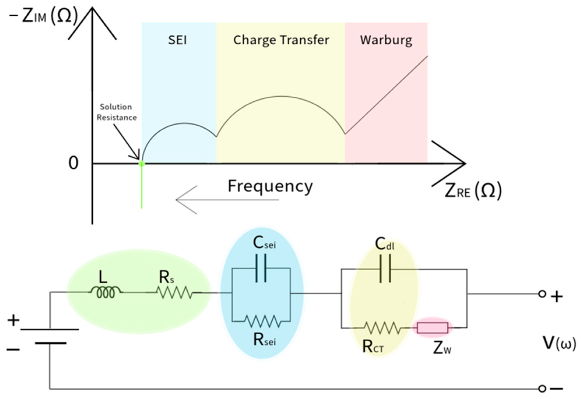
Potentiostats are the primary equipment used to acquire EIS spectra, which can measure the different kinetics within electrochemical devices ranging from under 0.001 Hz to over 1,000,000 Hz [10]. These spectra are best shown on a Nyquist plot (NP), which graphs the imaginary impedance vs. real impedance. The impedance on the NP shows that the real impedance (resistance) gets smaller at higher frequencies. It also shows that the kinetics observed at different frequencies can be viewed as a region where that phenomenon is the dominant contributor to the overall impedance in that region. A battery model used to provide an accurate simulation of the Nyquist plot for LIBs is an equivalent circuit model (ECM). This method uses electrical elements such as resistors and capacitors to describe the electrochemical behavior of an LIB’s EIS [11]. This method is helpful since it reduces the number of inputs to describe the EIS, making it less computationally expensive for battery health estimation. At very high frequencies where the impedance is below the Z_RE-axis, mutual inductance occurs between the connectors from the potentiostat and the cell’s connecting tabs [12]. At the intersection of the Z_RE-axis is the bulk resistance [13], where ions behave as resistors to impede electrons from flowing from the working electrode to the reference electrode, and this property can be attributed to the electrolyte, separator, and contact. At high frequencies, the impedance can be observed from the formation of the SEI layer, which displays both resistive and capacitive characteristics [14]. The mid-frequency region encompasses the overall charge transfer (CT) region, which includes the charge transfer resistance (R_CT) and double-layer capacitance (C_dl). The R_CT represents the opposition of Li⁺ traveling between the electrolyte and the electrode [15]. At the same time, when Li⁺ is adsorbed on the electrode, a space is formed between the electrode and the electrolyte interface. The system has capacitive characteristics, showing charges on both the electrode and electrolyte with a space in between [16]. The impedance at very low frequencies is observed through species moving from one electrode to the next, which is denoted as the Warburg diffusion [17]. 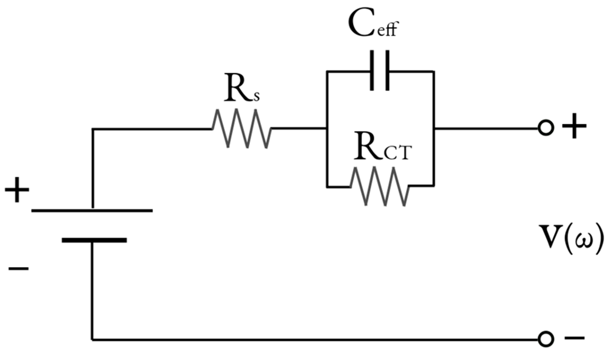Several models are used to model EIS, the most basic of which is the Thevenin model [18]. This model is used to capture the bulk resistance and the overall capacitive and resistive sections if the presence of the SEI is not apparent. However, it does not capture the diffusion spectra or consider the non-ideal capacitive behavior within the cell, so more advanced models for EIS modeling for LIBs are needed. One recent model useful for LIB approximation to obtain a global spectrum is the adaptive Randles ECM (AR-ECM) [19]. The nuance of the AR-ECM is that the Warburg impedance is placed in series with the R_CT. This considers the mass transport effect that is influential in the mid-frequency region. This is shown in Figure 1, which is used to simulate the EIS of an LIB. The associated parameters of ECMs are used in battery health studies as input to predict performance metrics, including state-of-charge estimation [20], state-of-health estimation [21], and remaining useful life estimation [22].

The accuracy of the equivalent circuit parameters (ECPs) from the ECM is essential for battery health prediction. Merrouche et al. investigated ECP estimation using artificial intelligence with the weighted mean of vectors algorithm as its foundation [23]. This method outperformed other state-of-the-art optimizers in convergence and speed metrics for ECP estimation and could predict unseen voltage data from its generated ECPs. Heydarzadeh et al. analyzed different modeling techniques to develop different ECPs depending on the battery’s chemistry [24]. For battery prognosis studies, recent work showcased the different avenues for estimating ECPs that were used for data input. Shao et al. accurately predicted the capacity of batteries using parameters associated with the SEI, showcasing that the global impedance spectrum is unnecessary to predict battery degradation [25]. Li et al. proposed a new ECM with three distinct time constants, with the Warburg parallel to a capacitor at the low-frequency spectrum [26]. They could accurately predict SOH, with an average root mean square error (RMSE) of 1.77%. Rodriguez-Cea et al. used only the internal resistance (R_int) model as input for SOH prediction [27]. The predictions of SOH fell between 2% and 5% of the measured SOH. Despite the diversity in methods using ECPs with various machine learning algorithms (MLAs) for battery prognosis, there is not much focus on using one LIB for model training and testing. Using one LIB for model building requires fewer resources for study in terms of experiment time and costs. This method also provides an alternative to conventional methods used in the literature by using simulated cells to predict their inputs and outputs based on EIS and capacity data, with uncertainties in measurement filtered by the equipment used to acquire EIS.

This study investigates the quality of ECPs for capacity prediction while providing a time-effective method to limit the time taken to acquire EIS and model training, showing usefulness in real-time SOH monitoring. A reduced equivalent circuit model is developed to estimate the ECPs in the high- and mid-frequency regions (R-ECM). These ECPs are input into a back propagation neural network (BPNN) to predict the simulated cells’ capacity. This algorithm is used over other algorithms, such as random forests and gradient boosting, that typically incur a long learning and running time for accurate results [28]. An effective R-ECM is used to replace the CPE with an effective capacitor to compare its ability to predict the capacity of cells (ER-ECM). Further analysis is performed to evaluate the usefulness of using singular ECPs within the ECM for capacity prediction. This method is compared to using the ECPs for all frequencies in terms of capacity prediction and time taken for model training and testing. Section 2 of this paper covers the methodology. Section 3 of this paper covers the results and discussion. Section 4 concludes this paper.

2. Methodology

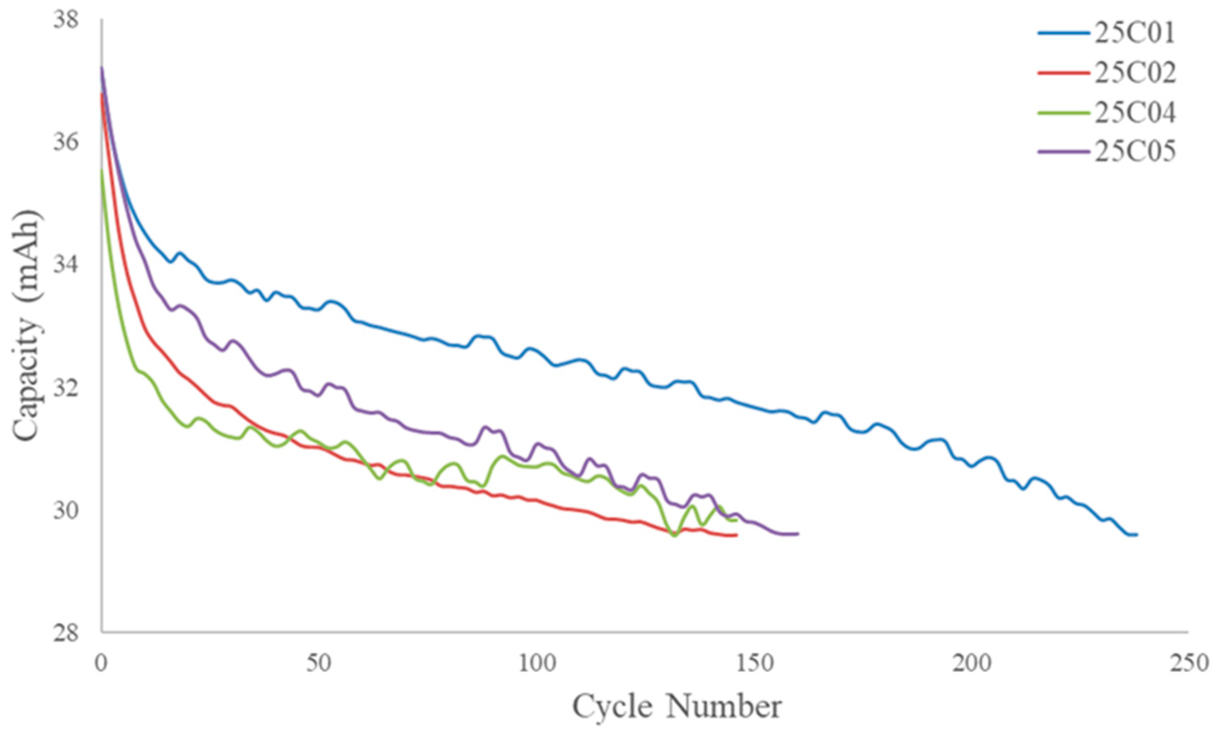
The dataset used for this study includes EIS and its corresponding capacity data for every even cycle in the cycle life of four LCO coin cells [29]. The dataset contains EIS for multiple stages during the charge/discharge cycle; however, the EIS data curated for this study were chosen 15 min after reaching 100% SOC. This was chosen so that the relaxation effect within the cell would slow to a negligible level so that it would not contribute to the overall EIS [30]. The data for each cell range from its initial cycle to the cycle closest to its end of life (EOL), which is when the cell reaches 80% of its initial capacity. This ensures that predictions are taken within the operating lifetime. Figure 2 shows the capacity retention curves for the cells in this study, and the equations for SOC and EOL are presented below, where Q_curr is the current capacity of the cell.

Table 1. Overview of cells used for analysis.

Cell ID	Cycle Life (Cycles)	Max Capacity (mAh)	Min Capacity (mAh)	Final SOH (%)
25C01	238	37.20	29.60	79.6%
25C02	146	36.77	29.59	80.5%
25C04	160	35.53	29.83	83.4%
25C05	164	37.21	29.59	79.5%

gives an overview of each cell’s capacity and cycle life.

SOC = (Q_curr/Q_max) × 100%,

(3)

EOL = Cycle_80%SOH

(4)

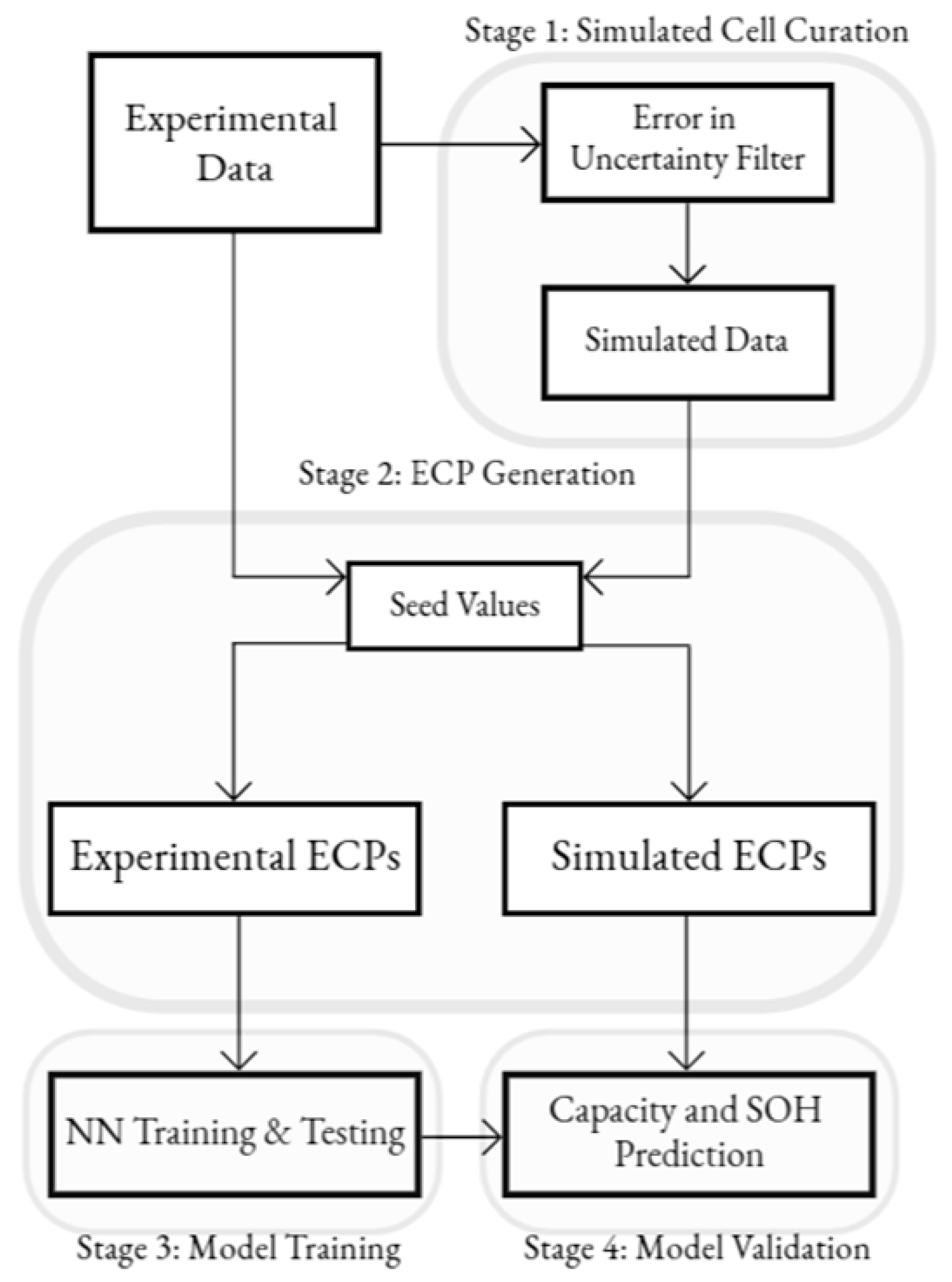
The overall framework of this study is shown in Figure 3. The EIS and the corresponding capacity data are run through an error-in-uncertainty filter to provide simulated data to predict each cell. This filter is based on the errors in uncertainty in measurement from standard potentiostats. The Gamry 600 was used as the testbench, which is ±1%, given the range of EIS values in the dataset. The capacity filter was set to ±1.5% for this study. The ECPs were acquired from the ECM used in this study, using appropriate seed values for the experimental and simulated data. The experimental ECPs (E-ECPs) were used as input into the BPNN to train the model to be tested on the simulated ECPs (S-ECPs) to predict the capacity of the simulated cell. This study investigated the high and mid-frequency regions of the EIS using all ECPs in the model used. This was compared to the method of reducing the CPE to an equivalent capacitance (C_eff), an alternative method for characterizing the CPE using one variable instead of two. Lastly, analysis was performed using individual ECPs and their correlation to predict battery degradation.

The ECM used to obtain the ECPs was a one-time-constant (OTC) Thevenin model using the constant phase element to describe the double-layer capacitance (C_dl). This choice was made due to the non-ideal observation of the capacitance in EIS. It is equated below with ω being the angular frequency, Y₀, and n being the characteristic parameters of the impedance [31]. Figure 4 provides a visual representation of the ECM used to acquire the ECPs in this study. The OTC was used in this study because of the nature of the cells selected. The presence of the SEI was not apparent in the NPs, and the bode plot, which shows the phase angle of the impedance (arg(Z)) vs. the frequency, only shows one Gaussian bell curve, which supports using only one OTC for the overall charge transfer region. Figure 5 shows the bode plots for all four cells, highlighting the one Gaussian bell curve for each cell.

Z_CPE = 1/Y₀(iω)ⁿ

(5)

To obtain ECPs from the ECM, appropriate initial values are needed to attain a good fit for the ECM. These are called seed values, and they generally need to be within two decades of the best-fit values to obtain a good fit [32]. Since EIS is non-linear, a non-linear least-squares fitting technique is required to obtain the ECPs. 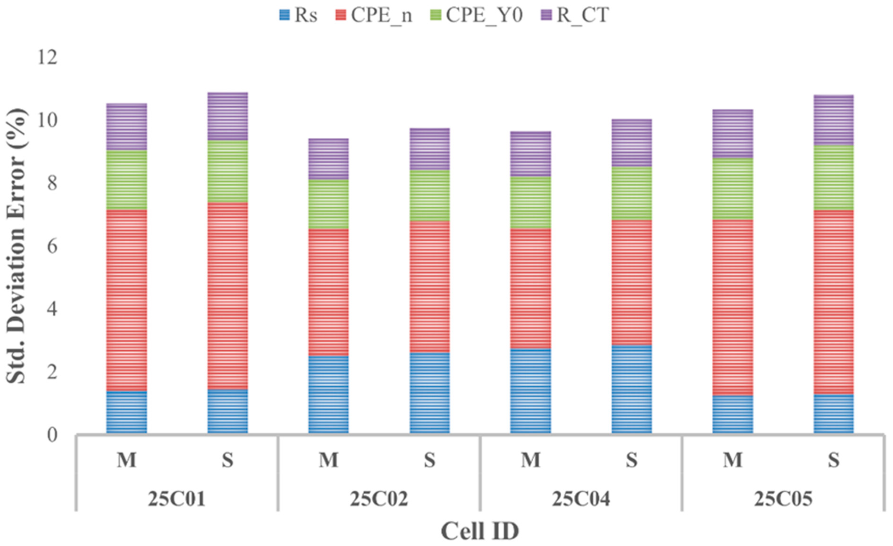Modeling programs for fitting an ECM to EIS data use the Levenberg–Marquardt technique [33]. The average values of the ECPs obtained for the four cells are shown in

Table 2. Average values of ECPs for experimental data.

Cell ID	Rs[Ω]		RCT[Ω]		CPE(n)		CPE(Y0)
	Value	$\pm$std	Value	$\pm$std	Value	$\pm$std	Value	$\pm$std
25C01	0.37	0.005	0.76	0.003	0.054	0.010	0.56	0.011
25C02	0.27	0.007	1.3	0.002	0.054	0.008	0.49	0.017
25C04	0.25	0.007	1.42	0.003	0.071	0.008	0.46	0.020
25C05	0.41	0.005	0.74	0.004	0.066	0.010	0.53	0.011

, along with their associated standard deviation errors.

Table 3. Average values of ECPs for simulated data.

Cell ID	Rs[Ω]		RCT[Ω]		CPE(n)		CPE(Y0)
	Value	$\pm$std	Value	$\pm$std	Value	$\pm$std	Value	$\pm$std
25C01	0.37	0.005	0.76	0.003	0.054	0.011	0.56	0.012
25C02	0.26	0.007	1.3	0.002	0.054	0.008	0.49	0.017
25C04	0.25	0.007	1.42	0.003	0.071	0.008	0.46	0.021
25C05	0.41	0.005	0.74	0.004	0.066	0.011	0.53	0.012

provides the ECPs for the simulated data. These errors were obtained at the 95% confidence level. The std. errors obtained are considered a good fit since they are less than the estimated parameter value, i.e., less than 100%. The root mean squared error (RMSE) of the initial values of each cell provides insight into the accuracy of the ECPs’ ability to predict the EIS spectra. They range between 0.0118 and 0.0173 Ω, showing negligible deviation from the impedance of the cells. Figure 6 shows all the cells’ average cumulative E-ECP and S-ECP deviation errors. The cumulative errors show that the ECPs acquired are of good fit and are usable for further study in predicting the capacity of the simulated cells.

$$RMSE=\sqrt{{\displaystyle \frac{{{\displaystyle \sum }}_{i=1}^n{\left({\hat{y}}_i-y_i\right)}^2}{n}}}$$

(6)

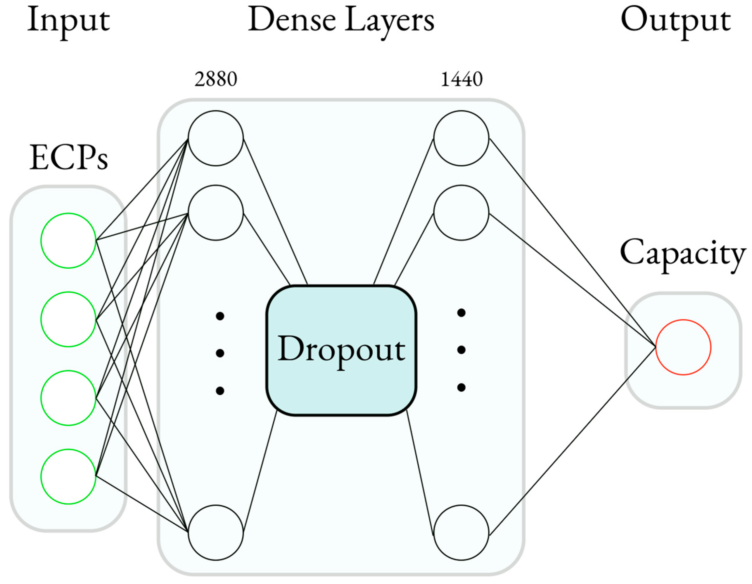
This study used a BPNN model as the machine learning algorithm due to its scalability and fast implementation. After acquiring the E-ECPs and S-ECPs, the E-ECPs were used for training and testing, with the E-ECPs as the input and the capacity as the output. The model was then used to predict the simulated capacity using the S-ECPs. Figure 7 gives an overview of the BPNN used, and

Table 4. Hyperparameters of the BPNN.

Hyperparameter	Value
Input Layer	No. of ECPs used
First Hidden Layer	2880
Dropout Layer	0.2
Second Hidden Layer	1440
Activation Function	relu
Output Layer	1
Optimizer	Adam
Loss Function	mean absolute error
Batch Size	16
Epochs	500

shows the hyperparameters used for the BPNN.

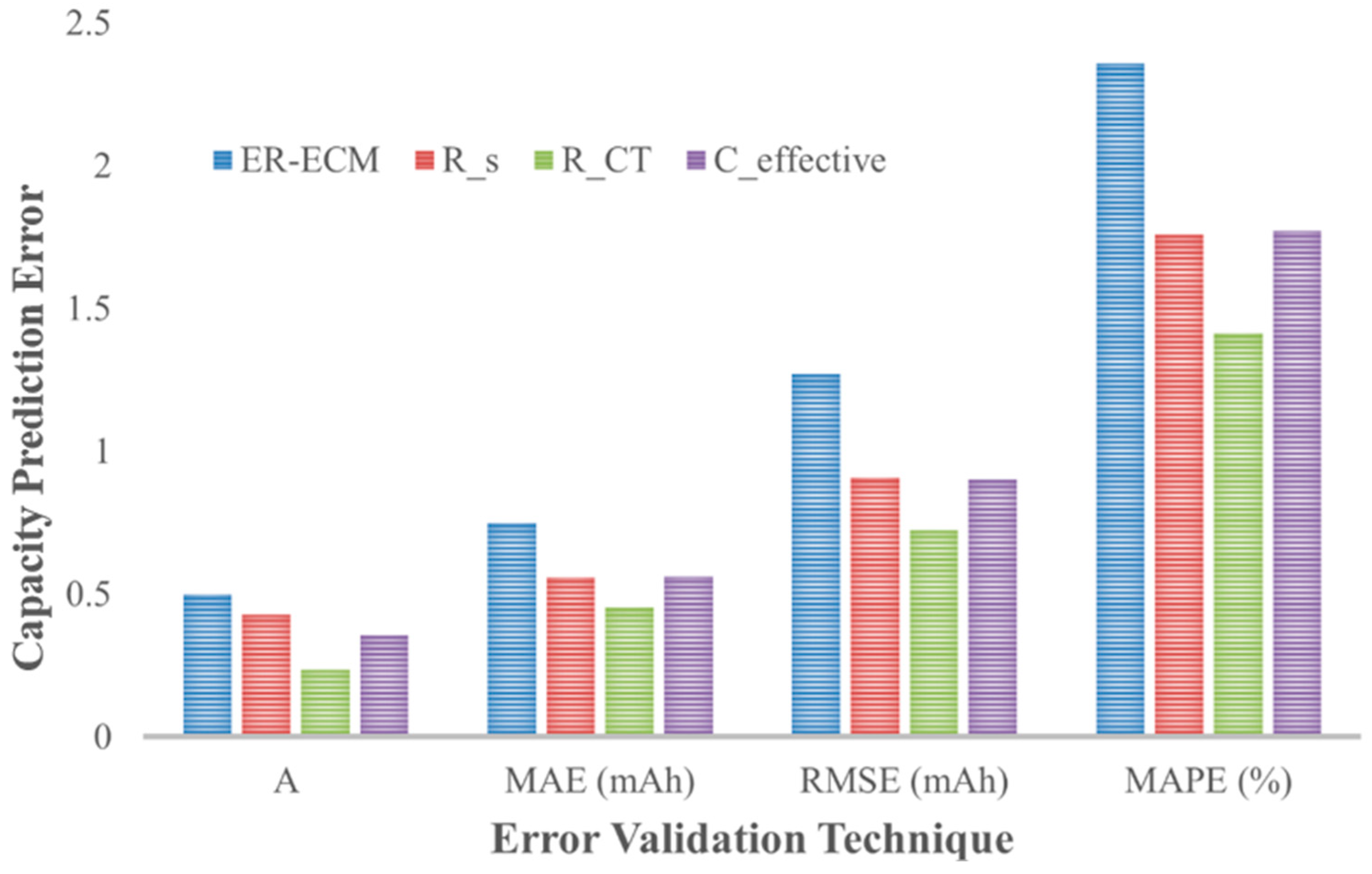
The simulated cell’s capacity prediction was evaluated using several error validation techniques, namely, the mean absolute error (MAE), the coefficient of determination (R²), the RMSE, and the mean absolute percentage error (MAPE). The MAE, R², and MAPE formulae are presented below, where y is the simulated capacity and ŷ is the predicted capacity from the S-ECPs. This combination of error validation techniques provides an exhaustive understanding of the robustness of the BPNN in predicting the capacity, where one technique may provide insight that others may not.

$$MAE={\displaystyle \frac{1}{n}}{{\displaystyle \sum }}_n^1\left|\left.y-\hat{y}\right|\right.$$

(7)

$$R^2=1-\left({\displaystyle \frac{{{\displaystyle \sum }}_{i=1 }^n{\left(y_i-{\hat{y}}_i\right)}^2}{{{\displaystyle \sum }}_{i=1 }^n{\left(y_i\right)}^2}}\right)$$

(8)

$$MAPE={\displaystyle \frac{1}{n}}{{\displaystyle \sum }}_n^1\left|\left.{\displaystyle \frac{y-\hat{y}}{y}}\right|\right.$$

(9)

To observe individual ECPs and their contribution to cell prediction, the CPE was converted into an effective capacitance, C_eff [34]. This was calculated according to Equation (10), where Y₀ is the admittance of the CPE, and n is a parameter used to describe the partial rotation of the depressed semicircle, with n = 1 indicating no depression, and a reduction in n describes an increase in rotation when it gets closer to 0. This reduced model is shown in Figure 8. This method reduces the CPE, a function of two parameters, into one, providing a pathway for measuring the C_dl using one parameter.

$$C_{eff}={\displaystyle \frac{{\left(Y_0{R}_{CT}\right)}^{\frac{1}{n}}}{R_{CT}}}\sin \left({\displaystyle \frac{n\pi }{2}}\right)$$

(10)

3. Results

3.1. Capacity Prediction of Simulated Cells

Using the E-ECPs as input into the BPNN, the capacity prediction of all simulated cells is shown in

Table 5. Capacity prediction of the simulated cells using the R-ECM.

Cell ID	R2	MAE (mAh)	RMSE (mAh)	MAPE (%)
25C01	0.44	0.95	1.83	2.91
25C02	0.81	0.39	0.71	1.24
25C04	0.39	0.72	1.1	2.32
25C05	n/a	2.76	4.15	8.78

. The value ‘n/a’, shown for R² evaluation, is due to the inability to find a correlation between the predicted capacity and the simulated data over the life cycle of the cell. For future analysis, this value is equated to 0. This method shows more robust predictions than using the full spectrum for capacity prediction, which includes the Warburg impedance, as shown in

Table 6. Capacity prediction of the simulated cells using the ECM including diffusion spectra.

Cell ID	R2	MAE (mAh)	RMSE (mAh)	MAPE (%)
25C01	0.42	0.62	1.04	1.94
25C02	0.16	1.43	2.55	4.57
25C04	0.16	1.12	1.62	3.60
25C05	n/a	1.95	2.76	6.23

. This is especially evident for cells 25C02 and 25C04, where the R-ECM shows significantly better predictions. This demonstrates the usefulness of reducing the ECM by removing the need for diffusion spectra, which is also the most time-consuming aspect of EIS acquisition. This indicates that researchers can reduce the time needed to obtain impedance spectra while obtaining similar or even better results for the same dataset.

Figure 9 shows the capacity and SOH retention curves for S25C02. The simulated curves are in blue, and the predictions are in red. Table 6 shows the predictions for the effective model. Three cycles are of note as they provided outlying predictions for S25C02. These are cycles 44, 50, and 110. Further analysis provided inconclusive theories on why these cycles provided higher capacities than the trend.

Table 7. Capacity prediction of the simulated cells using the ER-ECM.

Cell ID	Capacity Prediction of Effective Model
	R2	MAE (mAh)	RMSE (mAh)	MAPE (%)
25C01	0.85	0.38	0.62	1.03
25C02	0.79	0.39	0.65	1.24
25C04	0.36	0.69	1.18	2.24
25C05	n/a	1.54	2.64	4.92

shows an increase in the robustness of the BPNN in predicting the capacity with C_eff. The effective E-ECPs show significant improvement in predicting S25C01 and S25C05. The cells S25C02 and S25C04 show insignificant change. However, on average, the C_eff within the ECM is a better parameter for predicting capacity than the two parameters used for determining the CPE. This may be due to the use of only one parameter that provides a similar simulation of the charge transfer region as the CPE, which carries potentially less error than using the CPE for capacity prediction. This method, however, removes important surface heterogeneity information associated with the CPE. This is shown in Figure 10, with each error validation technique showing lower capacity predicted error results. In the case of the R² value, variable A is denoted to show the proportion of the variance of the predicted capacity that the model cannot explain. This is calculated as shown below:

$$A=1-R^2$$

(11)

3.2. Capacity Prediction of Individual ECPs

Since the ER-ECM provided higher-quality input than the R-ECM, it was used to evaluate the usefulness of the individual ECPs that comprise the model: R_s, R_CT, and C_eff. The BPNN described in Section 2 was used for consistency, and the results show that the R_CT provides the most robust results for capacity prediction. This can be attributed to the degradation patterns, such as the growth of the SEI layer with cycling. This is visualized in Figure 11 for cell 25C01, where the Nyquist plot shows the increase in the charge transfer region and more pronouncement in the SEI at its EOL.

Table 8. Capacity prediction of the simulated cells using the parameters of the ER-ECM.

Parameter	A	MAE (mAh)	RMSE (mAh)	MAPE (%)
Full	0.5	0.75	1.2725	2.3575
Rs	0.4275	0.5575	0.9075	1.76
RCT	0.235	0.4525	0.7225	1.4125
Ceff	0.3575	0.5625	0.9025	1.77

shows the average predicted capacity error for each ECP across all cells compared to that of the entire ER-ECM. The work conducted in [27] adds some validity to this observation, where the authors accurately and effectively predicted the SOH by using the internal resistance as input. This is shown in Figure 12.

3.3. Time Taken for BPNN Training and Testing

Table 9. Time elapsed for BPNN training and testing.

Cell ID	Time Elapsed (Seconds)
	All EIS Spectra	R-ECM	ER-ECM
25C01	82.99	78.98	78.41
25C02	57.38	53.33	51.17
25C04	54.06	51.07	51.31
25C05	62.66	58.81	58.73
Average	64.27	60.5475	59.905

compares the time for NN training and testing for all cells. The first item to note is that the time elapsed for each cell is reflected in the number of cycles, as shown in Figure 1 in Section 2. The second item to note is that the average time for training and testing decreased from using all frequency data to train to using the R-ECM and the ER-ECM with a lower number of inputs. The number of frequencies used in this dataset consists of 60 points of real and imaginary impedance, resulting in 120 inputs. The R-ECM consists of four inputs, and the ER-ECM consists of three. There is not much difference in the time elapsed. However, the ECMs provide faster training and testing by close to 6% than using the impedance spectra.

4. Conclusions

This study shows that using the impedance associated with the charge transfer resistance is effective for predicting the capacity of a cell, resulting in a 40% decrease in error prediction of capacity compared to using all the parameters of an ECM. This negates the need to model EIS spectra using all frequencies; only the key components from the high-frequency solution resistance and the kinetics that occur in the mid-frequency charge transfer resistance and double-layer capacitance are used. This work achieves accurate capacity and SOH predictions and introduces the possibility of using multiple batteries to train and predict an entirely new experimental cell. Since this research exclusively used LCO coin cells, future work should apply the proposed method to investigate other LIB chemistries and establish factors for generalizing LIB health predictive modeling. Adding multiple time constants to this model to account for the SEI’s influence on impedance can be applied for batteries that exhibit a strong SEI presence. Other future work for this approach includes understanding the differences between the high- and mid-frequency phenomena and their contributions to predicting the capacity of cells.