Simulation of Dendrite Growth with a Diffusion-Limited Aggregation Model Validated by MRI of a Lithium Symmetric Cell during Charging

Abstract

Lithium metal batteries offer high energy density but are challenged by dendrite growth, which can lead to short circuits and battery failure. Multiple models with varying degrees of accuracy and computational cost have been developed to understand and predict dendrite growth. This study presents a simple model to simulate macroscale dendrite growth on lithium metal electrodes. The model uses a 3D single-particle Diffusion-Limited Aggregation (DLA) algorithm with an electric field bias to simulate dendrite growth. The electric field bias was introduced into the model with an important parameter, namely the biasing factor c, which determines the balance between diffusion and electric field effects. Before performing the simulation with the proposed model, the dendrite growth in a lithium symmetric cell during charging was measured by sequential 3D magnetic resonance imaging (MRI). These data were then used to validate the simulation, as the dendrite structure in each measured MRI time frame was used a starting point for a new simulation, the results of which were then validated with the measured dendrite structure of the next time frame. The best agreement between the simulated and measured dendrite structures using the overlap and displacement of deposition sites metrics was obtained at the biasing factor c = 0.7. This agreement was also good in terms with the fractal dimension of the dendrite structures. The proposed method offers a simple, accurate, and scalable framework for predicting dendrite growth over long deposition periods, making it a valuable tool for studying dendrite suppression under real-world battery charging conditions.

1. Introduction

The commercialization of secondary lithium metal batteries holds significant promise for advancing energy storage technologies due to their high energy density and specific capacity. However, the current issue hindering their widespread adoption is the formation of lithium dendrites during charging, which may cause short circuits and lead to thermal runaway [1]. This challenge is being actively addressed by exploring strategies to prevent dendrite growth, such as employing electrolyte additives [2,3,4,5], designing innovative anode surface modifications [6,7,8,9], using mechanical stress [10], and exploring new charging procedures [11]. Along with that, simulation models that grant a deeper understanding of the electrodeposition process are constantly evolving [12]. Successful mitigation of dendrite formation will result in safer, more efficient lithium metal batteries, potentially revolutionizing the energy storage industry and enabling the development of longer-lasting and more powerful portable electronic devices and electric vehicles, as well as better energy storage systems and electric vehicles with longer range.

Dendrite growth in lithium metal batteries is influenced by a combination of electrochemical and mechanical factors. At low current densities, lithium tends to grow from the base due to plastic flow of lithium, while at high current densities, growth occurs at the tip driven by the electric field [13]. The process begins with the nucleation of lithium, which then grows into elongated dendritic structures. A thin layer, called the solid electrolyte interphase (SEI), which is made up of various inorganic and organic compounds, inevitably forms on the lithium surface as a result of electrolyte breakdown. The growing structures experience stress due to molar volume changes and interaction with the SEI. Stress distributions within the dendrite lead to different growth behaviors. Compressive stresses at the base promote vertical growth, while localized stresses at the tips cause branching and bifurcation. The electric field and thus the current density is higher at the dendrite tips, enhancing tip growth and leading to high electric fields and current densities that further drive uneven electrodeposition [12,13]. Six growth regimes have been identified—thermodynamic suppression, incubation, base-controlled, tip-controlled, mixed, and Sand’s regime—each characterized by specific current density and size-dependent behaviors [13]. Understanding these regimes and the underlying electrochemomechanical interactions is crucial for developing strategies to suppress dendrite growth, thereby enhancing battery safety and performance.

Various advanced in situ and operando imaging techniques have been utilized to characterize dendrite growth. Optical microscopy, due to its accessibility and simplicity, allows real-time observation of lithium dendrite formation, though it is limited by spatial resolution. Confocal Raman microscopy provides insights into Li-ion concentration gradients and dendrite formation with sub-micron spatial resolution but struggles with poor temporal resolution [14]. Scanning and transmission electron microscopy (SEM, TEM) enable high spatial resolution imaging of dendrite structures and the solid electrolyte interphase (SEI), although electron microscopy requires vacuum conditions and can introduce beam damage [15,16]. X-ray-based techniques such as X-ray contrast imaging enable non-destructive, high-resolution imaging of dendrites within opaque materials [17]. Neutron imaging, while less common, provides depth profiling and three-dimensional (3D) visualization of dendrite growth [16]. Additionally, Nuclear Magnetic Resonance (NMR) and magnetic resonance imaging (MRI) have been used to study the structural and dynamic aspects of dendrite growth [18,19,20,21]. Despite the low temporal and spatial resolution of MRI for dendrite characterization, its major benefit is its non-invasive nature, requiring only that the battery housing be non-metallic. Each technique presents unique advantages and limitations, collectively contributing to a comprehensive understanding of lithium dendrite growth mechanisms.

The models for dendrite growth can be roughly divided into three categories: Brownian statistical models, electromigration-based models, and surface tension models. The Brownian statistics model family for dendrite growth simulations focuses on the stochastic movement of lithium ions and their deposition on electrode surfaces. These models simulate the Brownian motion of particles, incorporating probabilistic rules to determine ion interactions and deposition events. By modeling the random walk of ions influenced by thermal energy and electric fields, Brownian statistical models provide insights into the nucleation and growth of dendritic structures. For example, Aryanfar et al. (2014) explored dendrite growth using both pulse charging experiments and Monte Carlo simulations, finding that pulse charging could disrupt continuous growth and promote uniform deposition [22]. A study by Magan et al. provides a detailed explanation of how the surface reaction kinetics affect the resulting size distribution of the interfacial nanostructures after deposition [23]. Chen et al. (2023) investigated how surface energy anisotropy, nucleation spacing, and interfacial electrochemical driving force impact dendrite growth, concluding that smaller nucleation spacing and lower surface energy anisotropy inhibit dendrite formation and promote smoother deposition [24].

Chazalviel’s model describes lithium dendrite growth under high current densities, emphasizing electromigration and space charge effects. When current density is high, lithium ion concentration near the electrode drops to zero at Sand’s time, leading to a build-up of positive charge and a localized electric field. According to this model, dendrite tips grow at a rate similar to the anion drift velocity, highlighting the critical role of ion concentration gradients and electric fields in dendrite formation. The work of Chazalviel provided a theoretical framework for electromigration-limited dendrite growth, showing how high current densities lead to a depletion of lithium ions and subsequent space charge formation [25]. Later, the influence of electrolyte motion, variation in ion mobility, and diffusivity with ionic concentration, as well as the effect of polarization cycling, were recognized as necessary improvements of the model [26].

The surface tension model explains lithium dendrite growth by emphasizing the balance between surface forces and mass transport. The study by Barton and Bockris discusses the role of surface effects in the formation and growth of dendrites during the electrolysis process. They found that the presence of surface roughness and defects on the electrode can significantly influence the initiation of dendrite growth. These irregularities can act as preferential sites for nucleation, where the local electric field is enhanced, promoting the deposition of metal ions [27]. A paper by Monroe and Newman models dendrite growth in lithium/polymer cells, showing that dendrite propagation accelerates with time and current density, leading to cell shorting at current densities above 75% of the limiting current. Increasing interelectrode distance and lowering current density can delay failure, but surface forces and transport properties have minimal impact on growth under the studied conditions [28].

So far, much work has been carried out in terms of characterizing dendrites at small scales, and the mechanisms governing their growth are well understood. However, costly molecular dynamics and phase-field simulations are not practical for studying the evolution of dendrites on the large time scales that allow them to grow relatively large. In this study, a Diffusion-Limited Aggregation (DLA) model is presented to predict the macroscopic evolution of dendritic structures. The DLA model was originally introduced to describe the stochastic process of particle aggregation under limited diffusion that can be used to explain the formation of fractal structures observed in natural and experimental systems [29,30,31,32,33]. In its traditional form, DLA assumes that particles undergo random Brownian motion and irreversibly stick upon contact, resulting in a fractal aggregate with a characteristic dimension. In three-dimensional (3D) systems, DLA clusters are known to exhibit a fractal dimension of approximately D = 2.5, a property that is indicative of the scale-invariant nature of the growth process [34]. However, the electrodeposition process involved in lithium dendrite formation introduces complexities that go beyond simple diffusion. During electrodeposition, the movement of lithium ions is not solely governed by diffusion but is also significantly influenced by electromigration. The electric field, which is particularly strong near the tips of growing dendrites, plays a crucial role in determining the morphology and growth dynamics of these structures. The combination of diffusion and electromigration leads to anisotropic growth patterns, with dendrites preferentially extending in the direction of the electric field.

In this study, the proposed DLA model is extended by introducing a bias, which controls the effect of the actual electric field on motion of the particles and thus also affects the structure of the resulting dendrites. This modification positions the model as a hybrid of Brownian and electromigration-based models, thus enabling the model to more accurately incorporate the conditions present during lithium electrodeposition where electromigration is the dominant factor. The novelty of this study is also in the integration of MRI data on dendrite growth into the simulation process. The advantage of this was twofold; firstly, it enabled a more accurate calculation of the electric field in the lithium symmetric cell during its charging and thus a better calibration of the simulation, and secondly, it enabled the validation of the simulation. This investigation not only seeks to validate the applicability of the DLA model in the context of electrodeposition but also aims to contribute to the broader understanding of pattern formation under non-equilibrium conditions. By exploring the accuracy of the DLA model, we hope to enhance the predictive modeling of electrodeposition processes, providing insights that could lead to the development of more robust strategies for mitigating dendrite growth and improving the safety and performance of lithium metal batteries.

2. Materials and Methods

2.1. Sample Preparation

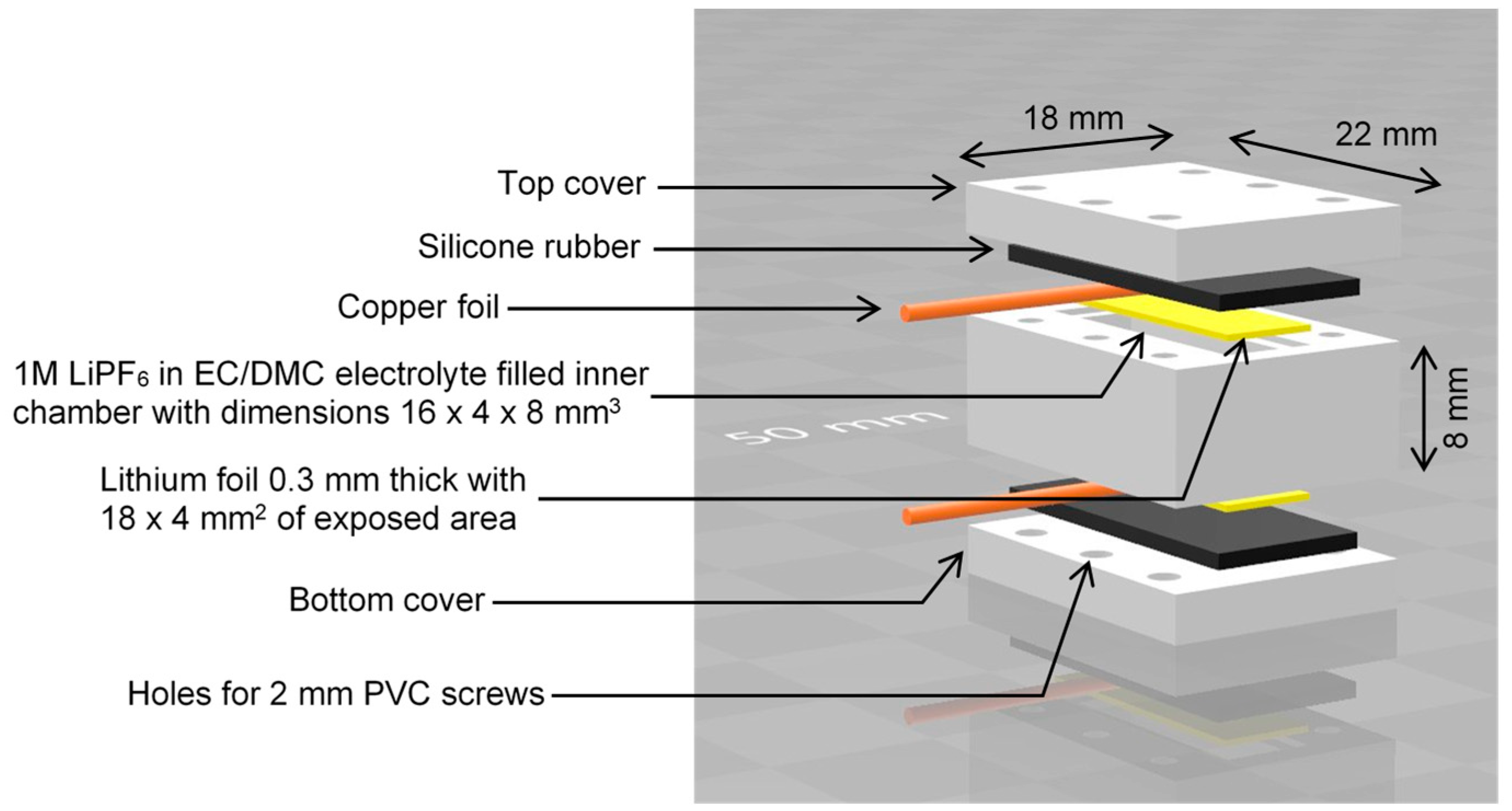
The model battery (lithium symmetric cell) was designed and assembled according to the scheme in Figure 1. The battery body components were made from PEEK plastic. For the electrodes, two rectangular, 0.3 mm thick lithium metal strips were cut from a roll of lithium foil. During assembly, the two electrodes were inserted into the recess provided for this in the main block, then covered with strips of a copper foil, which were used as current collectors, covered with silicone rubber gasket, and finally pressed from both sides to the main block with covers screwed on. This cell was filled with electrolyte through a small side hole, which was then sealed. The electrolyte was a solution of 1 M LiPF₆ in a 1:1 volumetric mixture of ethylene carbonate (EC) and dimethyl carbonate (DMC). The battery was assembled in an argon-filled glove box (Vigor Gas Purification Technologies, Marktheidenfeld, Germany).

2.2. MRI Experiments and Image Processing

The MRI experiments utilized a 9.4 T wide-bore vertical superconducting magnet (Jastec, Tokyo, Japan). The system was equipped with a Bruker Micro 2.5 gradient system (Bruker, Ettlingen, Germany) and operated under the control of a Tecmag Redstone spectrometer (Tecmag, Houston, TX, USA). Data acquisition was carried out using a 30 mm quadrature Bruker ¹H RF probe, which operated in a linear polarization mode.

For optimal magnetic resonance (MR) imaging, the cell was positioned within the magnet to ensure that the B₀ and B₁ magnetic fields were aligned parallel to the electrode surfaces. ¹H MR imaging of the battery was conducted using a 3D RARE sequence, with the following parameters: an inter-echo time (inter-TE) of 5.8 ms, a repetition time (TR) of 2030 ms, and an echo train length (ETL) of 8. The field of view measured 20 × 10 × 5 mm³ along the x, y, and z axes, and the data acquisition matrix was set to 128 × 64 × 32 in the read (x), first phase (y), and second phase (z) directions. This configuration provided a 3D image covering both the electrodes and the electrolyte region, with an isotropic spatial resolution of 156 μm.

Dendritic growth was monitored from the moment MR image acquisition began, with the battery cell subjected to a constant charging current of 1 mA throughout the experiment and a voltage cap of 4.0 V. Each imaging cycle took around 2 h and 20 min, followed by a 1 h pause before the next cycle. In total, 10 sequential images were captured, covering a complete experimental duration of 33.3 h.

The MR signal originates from the hydrogen atoms contained in the electrolyte [19], while the dendritic structure and other parts of the battery (housing, electrodes, leads…) do not produce an MR signal, as they do not contain hydrogen atoms. In addition, there is a number of interactions between the metallic dendrites and the electrolyte, such as magnetic susceptibility and RF shielding effects, which lead to a reduction in electrolyte signal. These complex interactions make it difficult to gauge their intensity and reach, meaning that the “signal void” does not necessarily represent the true shape of dendritic structures but only gives us a rough estimate that is generally larger than the actual dendritic structure [35].

The first step in image processing was to extract the 3D structure of the dendrite growth from the MR images. Initially, irrelevant areas of the images were trimmed to retain only the volume corresponding to the electrolyte region inside of the cell. Binary filtering was then applied using inverted thresholding, where voxels with values lower than the selected threshold intensity were set as 1, where these voxels represented dendrites, and other voxels were set as 0 and represented other parts of the battery. These binary images were then manually corrected slice by slice for each 3D image to address potential artefacts, gas bubbles, or other image imperfections.

2.3. Numerical Simulation

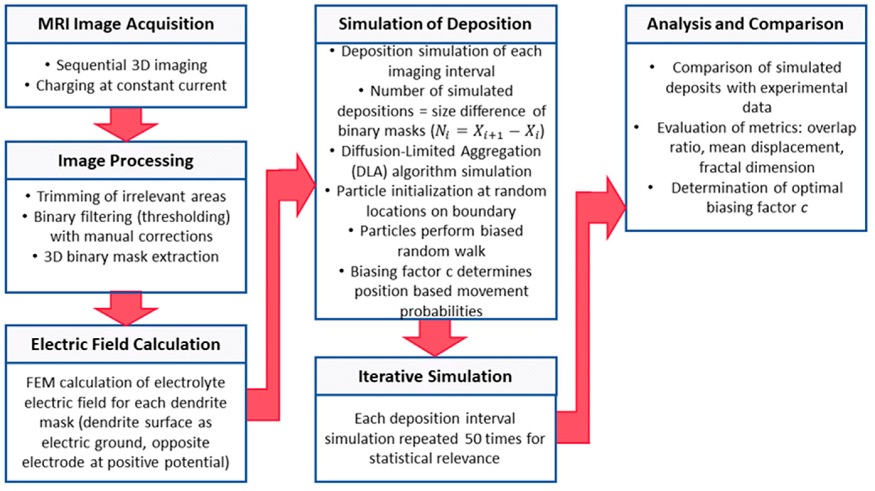
The simulation of dendrite growth followed the protocol shown in the diagram in Figure 2. Briefly, a sequence of ten 3D MR images was acquired first. These images were then used as a guide to simulate each of the nine deposition intervals, which were simulated in nine independent simulation steps using the same model but with different initial conditions. For each step, deposition sites were extracted. To increase the statistical relevance of the calculated deposition sites, each of the nine simulation steps was repeated fifty times. The simulation was performed on a grid representing the inside of the symmetric cell, with voxel dimensions matching those from MRI (156³ μm³). Given the cell size of 16 × 8 × 4 mm³, the grid size was 102 × 51 × 26.

Initial conditions for each simulation step were set based on binary 3D masks of dendrite structures extracted from MR images, labeling nonzero voxels as dendritic. First, the electric field was calculated for each 3D dendritic mask, with the surface of the dendritic electrode set as electric ground, while the opposing (flat) electrode surface had positive potential, and the surrounding walls were modeled as electric insulators. The current-to-next image deposition simulation used the initial conditions and the calculated electric field from the corresponding 3D dendritic mask. As the DLA model itself does not enable the determination of optimal simulation duration or current density to facilitate meaningful comparison with MRI data, it was ensured that the same number of sites were filled during the simulation as in the corresponding MR imaging interval. The DLA algorithm was then used to initialize each particle (dendritic voxel) at a random location on the domain boundary opposite the deposition electrode. The particles were subjected to a biased random walk, with the biasing factor c, determining the degree of bias against the electric field. If c is 0, the walk is unbiased (random); if c is 1, the particle moves only in the direction of the electric field. Motion probabilities were calculated from the electric field using the following equations:

$$\stackrel{\rightharpoonup }{E}=(E_x,E_y,E_z)$$

(1)

$$E_i^{norm}={\displaystyle \frac{\left|E_i\right|}{\left|E_x\right|+\left|E_y\right|+\left|E_z\right|}}\hspace{1em}\mathrm{for}\hspace{1em}i\in \left\{x,y,z\right\}$$

(2)

$$p_{i+}=\left\{\begin{array}{c}\frac{1}{6}+c\left(E_i^{norm}-\frac{1}{6}\right)\hspace{1em}\mathrm{if}\hspace{1em}{E}_i\ge 0\\ \frac{1}{6}\left(1-c\right)\hspace{1em}\mathrm{if}\hspace{1em}{E}_i<0\end{array}\right.$$

(3)

$$p_{i-}=\left\{\begin{array}{c}\frac{1}{6}\left(1-c\right)\hspace{1em}\mathrm{if}\hspace{1em}{E}_i\ge 0\\ \frac{1}{6}+c\left(E_i^{norm}-\frac{1}{6}\right)\hspace{1em}\mathrm{if}\hspace{1em}{E}_i<0\end{array}\right.$$

(4)

Here, $\stackrel{\rightharpoonup }{E}$ is the electric field vector, $E_i^{norm}$ is the electric field vector component of the normalized vector, and $p_{i+}$ and $p_{i-}$ are the motion probabilities of the particle in the positive and negative i direction, respectively. The simulation was performed for biasing factors c, ranging from 0 to 0.9, in steps of 0.1. For the purposes of statistical relevance for result analysis, each individual simulation was repeated 50 times. This gives a total of 4500 simulation runs (9 time intervals, 10 c-values, 50 repetitions).

The simulation was programmed in the Python programming language. Calculations of the electric field and current density were performed using the COMSOL Multiphysics software version 5.6 (COMSOL Multiphysics, Stockholm, Sweden). All simulations were performed on a standard PC with an Intel i7-1065G7 processor (Intel, Santa Clara, CA, USA), and only a single thread was used. The simulation runtime varied with the biasing factor c and was typically in the range of 2–5 min per iteration. With further optimization, this time could be significantly reduced.

2.4. Data Analysis and Validation

The optimal factor c was determined as the one that yields the best match between the dendrite structures in the experiment and in the simulation, measured using two different metrics. The first (overlap, o-value) metric is quite straightforward and is equal to the number of simulated deposition sites that overlap with the deposition sites measured by sequential 3D MRI (N_o), divided by the number of total deposition events (N_d)

$$o={\displaystyle \frac{N_o}{N_d}}$$

(5)

The second (mean displacement, s-value) metric is more complex. It corresponds to the mean displacement of the simulated deposition sites from the measured (actual) deposition sites. Specifically, for each measured deposition site, the distance to the nearest simulated dendritic voxel (d_i) is measured and normalized to the largest distance in the cell (space diagonal-d_s). These values are summed and divided by the total number of measured deposition sites (or of simulated ones, as this is identical). This metric provides a more comprehensive assessment of the simulation accuracy. For instance, even if the overlap fraction is low, the deposition sites might still be relatively close to the measured locations, indicating reasonable accuracy.

$$s={\displaystyle \frac{1}{N_d}}{\displaystyle \sum _{i=0}^{N_d}\frac{d_i}{d_s}}$$

(6)

Both metrics were calculated using the resulting 3D binary mask from each individual simulation run. The results were then averaged across 50 simulation runs and across all time intervals to provide mean values and associated standard deviations.

In addition to the two previously mentioned metrics, dendritic structures, simulated and measured, were also evaluated by the fractal dimension metric, which describes the complexity of a fractal pattern. In the context of dendritic growth, the fractal dimension provides insights into the branching nature and geometric complexity of the dendrites. The box-counting method was used to calculate the fractal dimension [36]. For each 3D binary representation of dendritic growth, the algorithm started by counting the number of occupied voxels with unit-sized boxes. The box size was then incrementally increased by one voxel until it matched the smallest side of the simulation domain. For each box size ϵ, the number of occupied boxes N(ϵ) was recorded. These values were plotted on a log-log scale $\log (N(\epsilon ))$ vs. $\log (1/\epsilon )$. The fractal dimension D was determined by fitting a linear regression to the log-log plot, with the slope of the regression line providing the fractal dimension

$$D=\underset{\epsilon \to \infty }{\lim }{\displaystyle \frac{\log (N(\epsilon ))}{\log (1/\epsilon )}}$$

(7)

The fractal dimension was used for validation once the model was calibrated. It was calculated for each individual 3D binary dendrite mask from the “optimum” simulation set, and then averaged across all time intervals and simulation runs. Standard deviations were derived from this averaging process. For the MRI experiments, the fractal dimension was computed from the filtered binary images, with the associated calculation error included to account for the signal-to-noise ratio of the images. The data analysis and validation processes were performed in the Python programming language.

3. Results

The entire dendritic structure can be optimally visualized by analyzing the evolution of the 3D binary mask extracted from MR images of the battery. The images in Figure 3a show the growth of dendrites in the central slice across the battery from 3.3 h (first image) to 33.3 h (last image) after the onset of battery charging. At 3.3 h, the electrode surface is visible with almost no dendritic growth. It appears that the electrode is slightly convex. At 6.7 h, the initial stages of dendritic growth are observable in the form of peaks, with minimal to no branching. As time progresses, more substantial branching and growth are evident. This pattern continues with the dendrites becoming more extensive and complex over the subsequent hours. Rapid growth is noticeable up to 26.7 h, and then with further growth the density of the structure only increases. By 30 h, the dendritic growth is substantial, nearly filling the available space. By 33.3 h, it has reached a highly complex and dense state. This progression highlights the continuous and extensive development of dendritic structures over time.

The first step before simulating dendrite growth was to calculate the electric field for the entire simulation domain, i.e., for each three-dimensional dendritic structure, as these data are used as input data for the simulation. A representative example of the calculated electric potential map and the corresponding current density map in a slice across the battery cell with dendrites is shown in Figure 4. The electric potential map in panel (a) provides a clearer understanding of the preferential direction of electromigration for a hypothetical particle located anywhere in the electrolyte. The potential is the highest near the top where the positive electrode is located and gradually decreases towards the bottom where the dendrites are present and the negative (grounded) electrode is located. The white areas in the maps represent dendritic structures. Areas with intense color changes correspond to areas of high electric fields. Since current density is proportional to the electric field due to uniform and isotropic electrolyte conductivity in the model, the electric field map would be equivalent to the properly scaled current density map in panel (b). The current density map has color-coded intensity, while the vector field indicates the direction of current flow. High current density regions are observed near the dendritic tips, shown in red, where the electric field is the highest. The vectors point towards these high current density regions, demonstrating how dendritic growth causes localized increases in current density and alters the overall current flow within the cell.

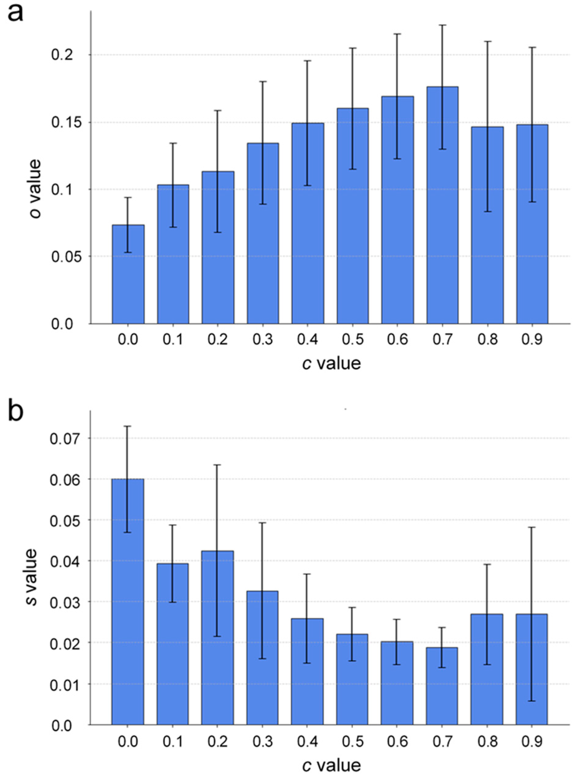
Figure 5 shows two bar graphs that were used to assess how well the simulated dendrites match with the actual ones at different biasing factor values c using two different metrics. The actual dendrites were extracted from 3D MR images of the battery cell, while the simulation results are represented by 50 simulation runs for the same set of simulation parameters, on which analysis is performed. Panel (a) shows the graph of the mean o-value in which the fraction of overlap between the actual dendritic voxels and the simulated ones is presented as a function of the biasing factor c, across all time steps for 50 simulation sets. The graph shows that the o-value generally increases with the biasing factor, peaking at around c = 0.7, and slightly declining after. Panel (b) shows a graph of the mean s-value, i.e., of the mean voxel displacement as a function of the biasing factor c, again, across all time steps for 50 simulation sets. The mean voxel displacement corresponds to the average distance from the actual dendritic voxel to the nearest simulated voxel, normalized to the volumetric diagonal of the battery cell. It can be seen that the displacement decreases as the biasing factor increases, reaching its lowest value at around c = 0.7. Lower mean voxel displacement signifies more accurate simulations, with simulated deposition sites closely matching the actual locations of dendrites. For the overlapping ratios (o-values), the standard deviation increases with c, while for the voxel displacement (s-values), the error bars show more variability. Despite this, the lowest absolute deviation and the smallest relative error appear to be around the optimal biasing factor. The graphs of both metrics show that a biasing factor of approximately c = 0.7 provides the best match between the simulation model and experimental data.

Figure 6 depicts the comparison between actual dendritic growth (left column) as measured by sequential 3D MRI and the corresponding simulated predictions (right column) of dendritic growth at matching times and for the biasing factor of c = 0.7. Each simulation shown was randomly selected from a set of 50 for the corresponding time point. The left column shows the actual dendritic growth as measured by MRI, while the right column displays the predicted deposition sites in the simulation that are overlaid (in red) on the dendritic growth from the previous MR image. The predicted deposition sites for all time intervals seem to align well with the measurements, indicating that the simulation adequately captures dendritic development. Overall, the comparison demonstrates that the simulation can effectively predict the most likely deposition sites between MRI intervals, providing valuable insights into the dynamics of dendritic growth in lithium metal batteries.

Dendritic growth is also known for its fractal structure. The fractal dimension can be considered as a measure of the complexity and branching nature of the dendritic structures. Therefore, the fractal properties of dendritic structures can be considered as one of the key properties for evaluating the quality of the presented model when simulating actual dendritic structures. Figure 7 shows a bar graph comparing the fractal dimensions of dendrite growth as a function of time for actual MRI-measured dendrites (blue bars) versus simulated dendrites (red bars). The fractal dimension of MRI-measured dendritic structures has an initial value around 2.25, which rises steadily with the deposition of lithium. However, between 10 h and 16.7 h, it plateaus before reaching a final fractal dimension of approximately 2.55. The simulation results align closely with the measurements, staying within the margin of error. For each time point, the majority of the 3D structure remains consistent, with variations only in the latest deposition sites. This consistency implies that the deviations from expected values are minimal, regardless of the biasing factor, especially when averaged over all 50 simulations. Notably, bar heights show strong similarity over time. The chosen optimal biasing factor of c = 0.7 results in fractal dimensions that closely match the experimental values across the entire range, demonstrating the accuracy of the simulation model. The results of this analysis could also suggest that the electrodeposition process under the given conditions can be described by 3D DLA universality class models, given that the fractal dimension hovers around the expected value of 2.5. However, such conclusions are preliminary, as the accuracy of the fractal dimension analysis is limited by the low spatial resolution of the simulation and imaging method used.

4. Discussion

The extension of the DLA model by electric field biasing is not new. It has been used in 2D simulations of electrodeposition [33,37]. However, the nature of the bias was simple as a uniform electric field was applied without considering its evolution during dendrite growth, thereby omitting a key factor influencing dendrite growth. In this study, this was considerably improved, as the electric field is now calculated based on the existing dendrite geometry and the particle motion is biased towards this field, making such an approach novel in DLA electrodeposition modeling. In contrast to direct molecular dynamics simulations, this model primarily focuses on the effects of electromigration and ion diffusivity within the electrolyte. Other factors, such as stress-driven lithium flow, solid electrolyte interphase (SEI) formation, surface diffusion, and evolving ion concentration profiles, are omitted to maintain model simplicity and computational efficiency.

MRI is particularly well-suited for this study, as it enables in situ, non-invasive imaging of dendrite growth during battery operation. This technique is crucial for monitoring dendrites in the high current density region, specifically within Sand’s regime. MRI enables continuous tracking of dendrite formation over extended deposition periods, often tens of hours, which is critical for understanding growth patterns under typical battery charging conditions.

Dendrite growth in lithium ion batteries, particularly in Sand’s regime, is significantly influenced by electromigration and ion diffusion. Electromigration drives lithium ions toward locations of the negative electrode with a higher electric field, causing localized ion accumulation and supersaturation at specific points on the surface of that electrode. This localized ion build-up creates nucleation sites for dendrites. On the other hand, the effect of ion diffusion is the opposite, leading to a more uniform ion distribution by migration of lithium ions from high-concentration to low-concentration regions. However, in Sand’s regime, the diffusion rate is insufficient to keep up with the rapid deposition of ions at the electrode surface, resulting in the formation of a depletion layer. This depletion exacerbates the conditions for dendrite formation by limiting lithium ion availability for uniform deposition, thereby promoting dendritic growth [25,26]. The competition between these two processes dictates the rate of dendrite growth: higher electromigration rates accelerate dendrite formation by continuously supplying ions to the growing tips, while inadequate diffusion fails to replenish the depleted regions, further facilitating dendrite elongation. For our simple model, a single parameter, the biasing factor c, encompasses the ratio of both effects; a higher value of c represents the domination of electromigration over diffusion. This parameter effectively captures the interplay between electromigration and diffusion, allowing us to predict dendrite growth rates under varying conditions. When c is high, indicating strong electromigration relative to diffusion, dendrite growth is rapid and more pronounced. Conversely, a lower c suggests that diffusion is more effective at mitigating the concentration gradients created by electromigration, thereby slowing dendrite formation. Consequently, the biasing factor c, together with the condition for the equal number of deposited particles (dendritic voxels) in the simulation and in the experiment, also affects the simulation time. In addition, the accuracy of this simulation also depends on the correct assumption of lithium density in dendritic voxels, i.e., the correct partition coefficient [35].

The simple model presented in this study could be of considerable value to future studies of lithium dendrite growth in lithium batteries, as it provides a computationally efficient method to predict the most likely deposition sites of lithium dendrites in Sand’s regime. Unlike more complex models, which may require extensive computational resources and detailed parameterization, this model simplifies the problem by using a single biasing factor c that represents the ratio of electromigration to diffusion effects. A higher c value, closer to 1, indicates a greater influence of electromigration, leading to faster and more pronounced dendrite growth, while a lower c value, closer to 0, suggests a stronger role for diffusion in mitigating dendrite formation. This model is particularly advantageous because it balances simplicity and accuracy, making it accessible for rapid iterative testing and refinement. By focusing on the biasing factor, the model can be quickly adjusted to match experimental conditions and predict dendrite growth patterns under various current densities and electrolyte compositions.

In this study, the model’s ability to predict the location and growth rate of dendrites with a reasonable accuracy was validated through comparisons with 3D MRI of actual dendritic structures. It is important to note that the characteristic size of features such as electrodeposited columns and branches ranges from 1 to 3 μm [17,38], whereas MRI’s spatial resolution in this study was approximately 156 μm. This disparity means the density of dendrites within each voxel is very low. The MRI signal originates from the electrolyte in the battery, and the impact of the presence of metallic objects on this signal is unpredictable due to the complex dependencies on the object’s shape and its orientation. Consequently, indirect magnetic resonance imaging is not ideal for characterizing dendrites on a microscopic scale but can still provide an insight into dendritic growth during battery operation on a macroscopic scale. The optimum biasing factor was determined by comparing the dendrite formation from 3D MRI and the corresponding simulation of the same process by comparing the deposition sites and mean displacements and the quality of the model by comparing the fractal dimensions obtained from MRI and simulations.

From the magnetic resonance images, a clear transition from dense column-like dendrites to highly branched structures is observed over time. This transition is quantitatively supported by the fractal dimension analysis. Fractal dimension in the context of dendrites quantifies the complexity and branching pattern of the dendritic structures. It indicates how the dendrites fill space, with a higher fractal dimension that corresponds to more intricate and highly branched growth. Figure 7 shows an initial plateau followed by a rise, indicating increasingly branched dendrites. Identifying the exact cause of this transition is challenging; however, several contributing factors can be considered. As dendrites grow, local current densities increase, leading to a higher overpotential at the eroding electrode due to the reduced surface area. Concurrently, concentration gradients become steeper as dendrites extend further into the electrolyte. This process is inherently self-accelerating: higher current densities at the tips of dendrites promote further growth, exacerbating the branching and complexity of the dendritic structures.

Some limitations of the model are evident. It is effective only when used alongside an imaging method. On its own, the model has limited utility, especially due to the lack of temporal information. The grid size is also too coarse for discussing “simulation particles”; it is more accurate to refer to deposition locations. However, as shown in both qualitative and quantitative analyses, this simple model has the potential to be a quick predictive tool when combined with a non-intrusive imaging technique, especially with further improvements. A novel aspect of our model is the use of calculated electric fields in conjunction with the DLA algorithm, unlike older models that assume a simple constant electric field. There is potential for further enhancements to improve the model’s accuracy or even make it suitable as a standalone tool for electrodeposition. Possible improvements include implementing a multiparticle model with surface diffusion, increasing computational grid resolution, and calculating electrolyte ion concentration and associated overpotentials.

5. Conclusions

This study presents the use of Diffusion-Limited Aggregation (DLA) algorithms enhanced with an electric field bias, which improved the model’s capability to simulate realistic dendrite morphologies. The resulting predictions align closely with experimental observations, demonstrating the model’s effectiveness in capturing the essential dynamics of dendrite growth. The presented model is distinguished by its simplicity, computational efficiency, and scale invariance, making it a very accessible method for predicting dendrite growth under typical battery conditions. It provides a reliable framework for predicting short-term deposition patterns without the complexity or computational demands of other models. As such, this approach offers a practical tool for researchers to explore strategies for dendrite suppression, such as optimizing electrolyte formulations or designing charging protocols, ultimately contributing to safer and more reliable lithium ion batteries.