A Genetic Algorithm Based ESC Model to Handle the Unknown Initial Conditions of State of Charge for Lithium Ion Battery Cell

Abstract

Classic enhanced self-correcting battery equivalent models require proper model parameters and initial conditions such as the initial state of charge for its unbiased functioning. Obtaining parameters is often conducted by optimization using evolutionary algorithms. Obtaining the initial state of charge is often conducted by measurements, which can be burdensome in practice. Incorrect initial conditions can introduce bias, leading to long-term drift and inaccurate state of charge readings. To address this, we propose two simple and efficient equivalent model frameworks that are optimized by a genetic algorithm and are able to determine the initial conditions autonomously. The first framework applies the feedback loop mechanism that gradually with time corrects the externally given initial condition that is originally a biased arbitrary value within a certain domain. The second framework applies the genetic algorithm to search for an unbiased estimate of the initial condition. Long-term experiments have demonstrated that these frameworks do not deviate from controlled benchmarks with known initial conditions. Additionally, our experiments have shown that all implemented models significantly outperformed the well-known ampere-hour coulomb counter integration method, which is prone to drift over time and the extended Kalman filter, that acted with bias.

1. Introduction

The development of batteries, especially their prolonged lifetime, increased capacity and high current charge/discharge abilities has accelerated the use of battery applications in many electronic and mechatronic devices. In the last decades, battery applications have been applied to areas of telecommunication devices, electric drives for electric and hybrid cars, as well as space probes. Battery management systems (BMS) [1,2,3,4] have played a crucial role in the safe and sound use of battery applications by (1) preventing the overcharging and overdischarging of batteries, (2) as well as monitoring and informing users regarding the state of the charge (SOC) and state of the health (SOH) of the battery cells. The two battery characteristics, i.e., the SOC and SOH, have been rigorously studied recently. The following methods are currently among the state-of-the-art for their determination and estimation:

• Direct measurement methods. These are as follows: the ampere-hour integral SOC estimation [5,6], open circuit voltage method, internal resistant method, electrochemical impedance spectroscopy, load voltage method, discharge test method, etc.
• Estimation method based on the black box battery model. Typical applications here involve machine learning (ML) methods, such as artificial neural networks (ANNs), support vector machines, genetic algorithms (GA), particle swarm optimization algorithms, fuzzy algorithms, deep learning methods, etc., to obtain the battery model from a large amount of input data for SOC estimation [7].
• Estimation method based on the state-space battery cell model. The original and adaptive Kalman filter (KF) versions are frequently found, such as extended KF [8], dual KF [9], unscented KF [10], adaptive KF [11], sigma-point KF [12]. Also, particle filters have been utilized in the past to adapt the model parameters due to battery cell temperature fluctuations and measurement noises [13].

Direct measurement methods do not require any modeling, as all necessary data are acquired through physical measurement. Some of these methods are invasive and irreversible, potentially causing permanent damage to the battery cell, while others are non-harmful. Black box battery models, based on statistical learning, are powerful and effective but traditionally require large amounts of data. These methods can also pose significant resource challenges when run on embedded hardware. In contrast, state-space battery cell models typically demand fewer resources. It is important to note that both black box and state-space battery models require some degree of measurement to run and monitor the surrogate model. Surrogate model-based methods are indirect; they need to be evaluated to estimate the SOC, unlike direct measurement methods, which provide the SOC directly. The following battery cell models are well-known among practitioners [7]:

• Electrochemical mechanism models (pseudo-two-dimensional models [14] and its simplified models, single-particle models [15], and the newest model, the most accurate model, the full homogenized macroscale model [16]).
• Equivalent circuit models (Rint model [17], RC model [17], Thevenin model [5,17], PNGV model [17], dual polarisation model [17], enhanced self-correcting model (ECM) [17,18], etc.).
• Data-driven models which mainly include neural network models, autoregressive models, and support vector machine models [7].

Despite their very high accuracy, electrochemical mechanism models have not been widely used in engineering applications for two main reasons: (1) the high complexity of the non-linear system with partial differential equations that lack analytical solutions, requiring significant computational power for numerical solutions, and (2) poor adaptability to certain working conditions. Equivalent circuit models have gained popularity for SOC engineering applications over the past decade due to their simple structure and parameter adaptability, despite their questionable accuracy and inability to reflect the internal characteristics of the battery cell. The popularity of data-driven models is rising, but they still require a large amount of input data to learn the battery cell model and achieve at least moderate accuracy.

Coulomb counting (CC) [17,19] is a widely used method for estimating the state of charge (SOC) of batteries due to its simplicity. It is reliable, but susceptible to integrator drift over time and variations in charging efficiency. The problem of integrator drift is traditionally addressed by frequent recalibrations at the battery’s maximum or minimum voltage when fully charged or discharged. However, such an approach is not always feasible as batteries may run without achieving these two extremes. Another problem of the CC is the charging efficiency. Namely, when charging, excessive heat may generated which can cause less than 100 percent of the charging energy to be stored into the battery. The enhanced Coulomb counting (ECC) method addresses this problem by introducing a parameter known as charging efficiency, denoted by $\eta$. The ECC will be used in the continuation of the study.

The Thevenin model is the most commonly employed ECM [20]. However, the Thevenin model is unable to address the nature of cell hysteresis due to the effects of charging and discharging. Hence, new versions of models like the Equivalent Circuit Model (ECM) emerged, with the Enhanced Self-Correcting (ESC) model being one of the most widely used ECMs today. Typically, two parallel pairs of RC circuits (2RC) are utilized rather than one pair (1RC), to  capture the rapid and complex cell dynamics better. Identifying the ESC parameters is called parameterization. To identify these parameters, the battery cell (or group of cells) needs to undergo a specific experimental test with numerous consecutive charging and discharging periods. This activates both the static and dynamic nature of the battery, varying its Open Circuit Voltage (OCV). The measured time lags in OCV can then be used to estimate the RC parameters. Knox et al. [20] compared several test profile identification methods. The more well-known non-invasive methods include the Galvanostatic Intermittent Titration Technique (GITT), Hybrid Pulse Power Characterization (HPPC), and Electrochemical Impedance Spectroscopy (EIS). In GITT, the cell undergoes a profile of short current pulses followed by relaxation periods [21]. Temperature, voltage, and current are monitored, and their dynamics are used for the parameterization of the ESC model. The most fundamental method of parameter identification is the non-linear least-square curve fitting method, where a higher-order polynomial is fitted. Customized test profiles are frequently practiced among researchers. A more coherent method is the Iterative Parameter Identification Algorithm (IPIA) [20]. Often, fitting is conducted using metaheuristic methods, where the penalty function is set as the squared deviation between actual and ESC-predicted voltage. HPPC involves monitoring the ratio of voltage drop to the current load applied, $\Delta V/\Delta I$, and deriving ohmic parameters from voltage drops. EIS, on the other hand, is a frequency-based identification method, rather than a time-based one like GITT and HPPC, making it somewhat more complex [22].

The Linear Kalman Filter (LKF) is another computation method for estimating the SOC, although its linear nature imposes several drawbacks. Practice shows that extreme values of SOC, i.e., below 10% and above 90%, are often difficult to estimate due to the very nonlinear nature of the cell (except 100%, which is called a maximum end voltage and is hence utilized for calibration purposes). This is because basic LKF is suitable only for linear systems with white and Gaussian noises, which is clearly not the case for the highly non-linear ESC model of a battery cell. The Extended Kalman Filter (EKF) corrects the cell nonlinearities to some degree by performing linearizations. Hence, EKFs are more suitable for such problems, contributing to their popularity among researchers [18,23]. A sample of these includes [24,25,26]. A drawback of the EKF is sometimes a burdensome convergence of the learning algorithm, as stated in He et al. [27]. As a result, various hybridizations of EKF emerged, such as adapting the battery parameters or covariance matrices. Yun et al. presented the idea of adapting the battery parameters in [28]. The authors adapted the battery’s internal resistance as well as the parameters of RC elements. Underlying various simulations have shown more accurate estimations compared to the classic EKF. Zhang et al. [29] implemented an adaptive EKF named AEKF, in which they adapted the measurement noise covariance and error covariance matrices. The authors reported that the estimation accuracy was better than using the classical EKF. Alternatively, ref. [30] implemented a hierarchical adaptive EKF, i.e., the HAEKF, where they split the state-space equation into two different submodels with two different sampling rates. One of these was intended to capture the lower dynamics, the other the faster dynamics. Experiments have shown greater reliability of such a method compared to the classic EKF.

The Sigma Point Kalman Filter (SPKF) [31] and Particle Filter (PF) [32] are other examples of a KF for estimating the SOC, even more advanced than the EKF. Furthermore, the SPKF can be easily adapted to enhance its performance below the SOC of 10% by including an H infinity filter [5]. This may be an accurate method. Authors in [16] compared the accuracies of two electrochemical mechanism models, i.e., the Doyle–Fuller–Newman model (DFN) and the full homogenized macroscale model (FHM). Parameters of both the models were obtained using particle swarm optimization (PSO), where 18 variables per model were involved. The FHM was shown to overcome the limitations of the DFN regarding the prediction of voltage responses at high temperatures. Another example of combining the PSO with the PF was published by Pang et al. [33].

The recursive least squares (RLS) is another example of a battery parameter estimator. It is a type of adaptive filter that rests on a weighted least squares regression method. Initially, the covariance matrix is initialized to a high value, and identified parameters are equal to 0. The forgetting factor $0<\lambda \le 1$ is introduced, where values close to 1 represent a focus on the new data points, and values close to 0 focus on the old data points. As the RLS recursively runs each time step, the identified parameters adapt in the way that the cost function, which represents the error between actual and predicted values, minimizes.

Ren et al. [34] show an application of the RLS for parameter identification of the lithium-ion battery. Authors argue that as the battery parameters are continuously adapted, the predicted value of a terminal voltage continuously approaches its true value. Liu et al. [35] employ a variable and adaptable window size within which the battery parameters are identified. The authors argue that too many data points too far away in the past may cause data saturation, which can act negatively on the correctness of identified parameters. Interestingly, they use RLS only for online parameter identification, while for estimating the SOC, they employ an unscented Kalman filter that runs in parallel. Ge et al. [36] employ an adaptation of the forgetting factor. They argue that the so-called improved forgetting factor RLS makes the parameter identification less prone to jitter and divergence under complex conditions. Li et al. [37] employed an RLS parameter identification under strong electromagnetic interference. Both the SOC and SOH were co-estimated using the UKF, here the SOH has been expressed as a ratio between estimated and rated capacities.

Recent trends within the state-of-the-art methodologies in the field include machine learning and deep learning approaches towards both the SOC and SOH predictions. Chen et al. [38] proposed the self-attention long short-term memory (LSTM-SA) for reliable and robust SOC estimations on different current profiles, temperatures and aging levels. Empirical experiments have shown clear LSTM-SA convergence to the unbiased estimate of the SOC with average errors within 2%. Li et al. [39] implemented a digital twin involving the LSTM and the convolutional neural network (CNN) for predicting the SOH. Predicted capacity errors of less than 3 mAh were observed. Reza et al. [40] implemented a hybrid LSTM where its hyperparameters are optimized using the lightning search algorithm (LSA). The authors argued that the hybrid LSTM-LSA outperformed the standard LSTM on the problem of remaining useful life (RUL) prediction. Dineva [41] and Madani et al. [42] published a thorough review of deep learning approaches toward reliable SOH predictions.

Our inspiration for this work was the ESC model, parameterized on an experimental training cycle, and utilizing the metaheuristic nature-inspired optimization algorithm (in our case, GA). The novelties of the paper are as follows:

• In the first proposed framework, a self-correcting feedback loop with an adaptable gain is proposed to obtain an unbiased estimate of the SOC. Initially, a biased initial condition of SOC0 is input externally, which then gradually with time converges to an unbiased estimate.
• The second proposed framework does not utilize a feedback loop as a first framework to realize the initial condition of SOC0 but rather estimates it as an additional GA dimension. The dimensionality of the GA problem thus increases from 9 to 10 independent variables.
• The adaptation of mutation probability (mutation rate $p_m$) is implemented. An average fitness performance is measured for the last generations and if no significant improvements are realized, the mutation probability is increased for the $p_m+\Delta p_m$. If no further improvements are realized the mutation probability is increased further, each time by $\Delta p_m$.

The proposed ESC model is realized in practice in less time than the classic ESC, as knowing the initial condition of SOC0 is not needed. This means that the operator does not have to run experimental tests to find one. Also, due to the existence of the feedback loop, the ESC performs in a more reliable way. Even if the initially set SOC0 is not correct and the bias exists, such bias is decreased automatically over time.

The structure of the paper is as follows: First, the materials and methods, including all three proposed techniques are presented. Next, the experiments and results follow. A reader may find practical evidence regarding the visual and statistical analyses of the results. Finally, the discussion is supplied.

2. Materials and Methods

Lithium Titanate Oxide cell (LTO) batteries are a type of battery with low self-discharge characteristics, high energy density, and relatively opportunistic recycling options [43]. The LTO is a graphite-free cell with anode chemistry formulae ${\mathrm{Li}}_4{\mathrm{Ti}}_5{\mathrm{O}}_{12}$ (titanate oxide nanocrystals). Lithium salt ${\mathrm{LiPF}}_6$ dissolved in an organic solvent acts as an electrolyte. Their working principle lies in a cathode full of lithium ions which are moved through the electrolyte to a titanate anode [44]. Charging the battery is called oxidation, and discharging reduction (lithiation of titanate oxide) [44]. Both the charging and discharging form a so-called redox cycle, with voltage (or SOC) slightly changing between minimal, nominal and fully charged. The OCV varies with respect to the SOC [1], the higher the SOC, the higher the OCV, and vice versa. Experiments and testings in this paper were executed utilizing the LTOs, with specification tag LTO1865-13, purchased from the company GWL a. s., Prague, Czech Republic. Crucial parameters of the LTO battery are presented in

Table 1. Specifics of the LTO battery cell utilized in the experiments.

Parameter	Value
Model name	LTO1865-13
Nominal voltage	2.4 VDC
Nominal capacity	1300 mAh
Minimal capacity	950 mAh
Max. voltage per cell	2.8 VDC
Min. voltage per cell	1.5 VDC
Standard operating voltage	1.85–2.75 VDC
Max. discharge current	<13 A @ 10 C
Max. peak discharge current	<26 A @ 20 C
Optimal discharge current	<1.3 A @ 1 C
Max. Charge current	<6 A @ 5 C
Optimal charge current	<1.3 A @ 1 C
Static charge or discharge current	≤43.33 mA @ C/30
Internal resistance	<20 m$\Omega$

.

The proposed work was based on three distinctive tasks (yellow, blue, and red), as outlined in Figure 1. The first task involved the identification of the battery cell, as suggested by [1]. Two different identification procedures were conducted: static and dynamic identifications, both represented by yellow rectangles. The OCV-SOC relationship was recorded as a static battery relationship, implying that the identification experiments of charging and discharging were carried out at a very low reference current rate, typically $i_{ref}=C/30$ or below [1]. The motivation for keeping the current that low was to avoid exciting dynamic elements within the battery. Next, the dynamic identification of the battery cell followed. This included rapid current changes while monitoring the transient phenomena. Extensive and durable battery tests and measurements were conducted for this first task. Following this, the training (or tuning) of the ESC model was performed. The objective of ESC tuning was to seek and find the optimal ESC parameters. Frequently, this was conducted using an optimization algorithm; we chose the Genetic Algorithm (GA). Here, three different frameworks of the ESC model were proposed and implemented, all utilizing the GA. These were named GA-ESC, GA-ESC+FB, and GA-(ESC+SOC0), where FB stood for feedback. Finally, laboratory experiments and testing were conducted to check the validity of the frameworks.

2.1. Static OCV Relationship of the Battery Cell

The identification of a static relationship OCV-SOC was conducted in a controllable test temperature chamber. The process was executed as suggested in [1]. First, the battery cell was placed at the ambient temperature of $T_a=-5 °\mathrm{C}$ and was fully charged. Next, the OCV-SOC nonlinear characteristics were recorded at discharging reference rate $i_{ref}=C/30$ until the battery was fully discharged. The ambient temperature was then increased by $\Delta T=5 °\mathrm{C}$ and the process was repeated. We continued this process until the ambient temperature reached $T_a=45 °\mathrm{C}$ (see Algorithm 1). Here, $i_{ref}$ represents reference (desired) current. Figure 2 depicts how the battery was connected to the testing platform.

Algorithm 1 SOC-OCV Recording with Temperature Variation

1: Initialize empty lists and monitor each time step: $T_a$, $SOC$, $OCV$0   2: Set initial temperature: $T_a\left[0\right]=-5 °\mathrm{C}$   3: Set temperature increment: $\Delta T=5 °\mathrm{C}$   4: Set maximal ambient temperature $T_{max}=45 °\mathrm{C}$   5: Start of SOC-OCV recording   6: while  $T_a\le T_{max}$  do   7:       Set and record temperature $T_a$   8:       Relax for 2 h              ▹ Remark: Relaxing the battery means $i_{ref}=0$ A.   9:       Discharge at $i_{ref}=C/30$ for 10 min 10:       Charge at $i_{ref}=C/30$ till $U_{batt}=V_{max}$ then relax for 2 h 11:       Discharge at $i_{ref}=C/30$ till $U_{batt}=V_{min}$ then relax for 2 h 12:       Charge at $i_{ref}=C/30$ for 10 min 13:       Discharge at $i_{ref}=C/30$ till $U_{batt}=V_{min}$ then relax for 2 h 14:       Charge at $i_{ref}=C/30$ till $U_{batt}=V_{max}$ 15:       Record corresponding SOC and OCV values at all times 16:       Increase temperature: $T_a\leftarrow T_{a-1}+\Delta T$ 17: end while 18: End of SOC-OCV recording 19: Output: $T_a$, $SOC$, $OCV$

The following OCV relationship was established [1] as shown in the following Equation (1):

$$OCV\left(SOC\right[k],T[k\left]\right)=OCV0\left(S0C\right[k\left]\right)+T\left[k\right]·OCVrel\left(S0C\right[k\left]\right),$$

(1)

where k represents the time sample and the $OCVrel\left(\right)$ is a temperature correction factor of $V/°\mathrm{C}$ [1]. Essentially, this equation calculates the OCV0 for a given SOC and corrects it for the underlying temperature (so that the calculation is valid for any underlying temperature).

2.2. Dynamic Relationship of the Battery

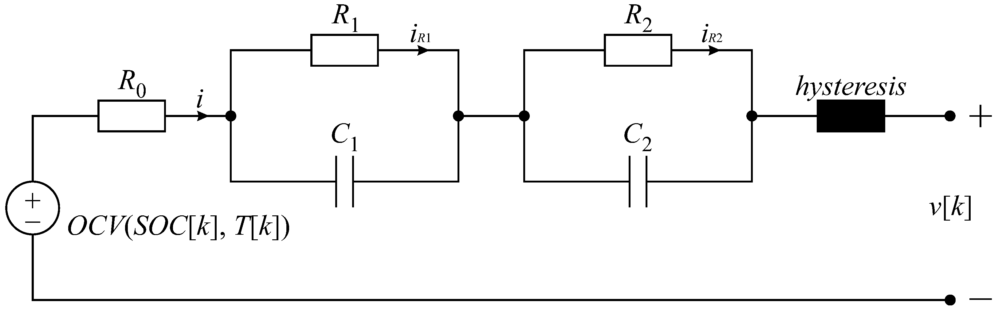
The dynamic relationship of the battery focuses on realizing the dynamics of the battery when undergoing abrupt and rapid changes in load. Figure 3 shows an equivalent RC circuit of the battery. The static relationship considers the voltage generator $OCV\left(SOC\right[k],T[k\left]\right)$ and the resistor $R_0$. The dynamic relationship considers the n-th parallel pairs of the RC elements and a hysteresis element [1]. The equivalent series resistance $R_0$ represents the voltage drop if the battery is being discharged and the voltage rise if the battery is being charged. The n-th RC parallel elements, which are wired in series, represent diffusion voltages that correspond to transient responses. Each RC element incorporates its time constant by capacitor $C_j$ being discharged through resistor $R_j$. A hysteresis element (black box in Figure 3) symbolizes the terminal voltage difference, depending on whether the battery has been recently charged or discharged. Several different types of battery hysteresis exist, among others voltage hysteresis, due to first-order phase transitions and kinetic pathways [45], battery resistance hysteresis due to aging [46], and temperature-dependent hysteresis due to ambient temperature $T_a$ [47]. Plett et al. [1] in the classic ESC model consider the voltage hysteresis only in two different types, i.e., the SOC-varying hysteresis $h\left[k\right]$ and instantaneous hysteresis $s\left[k\right]$. The first type describes changes in hysteresis with respect to the SOC, while the second type describes voltage jumps at a constant SOC if the direction of current flow changes. Two additional dimensionless parameters to be tuned were supplied here, i.e., M and $M_0$, where the final hysteresis voltage, denoted as $hyst\_volt\left[k\right]$ in Figure 3, is calculated as their sum.

2.3. Synthesis of the ESC Model

The ECC model is defined as follows in Equation (2) [1]:

$$SOC[k+1]=SOC\left[k\right]-{\displaystyle \frac{\Delta t}{Q_{total}}}·\eta \left[k\right]·i\left[k\right],$$

(2)

where $Q_{total}$ represents the total capacity, $\Delta t$ the time sample, $\eta \left[k\right]$ the Coulombic (charge) efficiency, $i\left[k\right]$ the current in given k-th time step. The direction of the current $i\left[k\right]$ can be either positive or negative, where positive current represents discharging and negative current represents charging the battery cell [1].

Let the $F_j$ represent the rate factor of the j-th RC circuit as $F_j=exp\left(-{\displaystyle \frac{\Delta t}{R_j{C}_j}}\right)$, where $j=1,2,\dots ,n$, and let the ${\mathbf{i}}_R\left[k\right]$ represent the current vector of currents flowing through each RC element. Let the $i\left[k\right]$ be a current (scalar quantity) flowing through the $R_0$. Then, a forthcoming state of the current vector ${\mathbf{i}}_R[k+1]$ can be predicted as follows:

$$\begin{array}{cc}\hfill {\mathbf{i}}_R[k+1]& =\underset{\left(A_{RC}\right)}{\underbrace{\left[\begin{array}{ccc}{F}_1& \cdots & 0\\ ⋮& \ddots & ⋮\\ 0& \cdots & F_n\end{array}\right]}}·{\mathbf{i}}_R\left[k\right]+\underset{\left(B_{RC}\right)}{\underbrace{\left[\begin{array}{c}\left(\begin{array}{c}1-F_1\\ 1-F_2\\ ⋮\\ 1-F_n\end{array}\right)\end{array}\right]}}·i\left[k\right],\hfill \end{array}$$

where $A_{RC}$ and $B_{RC}$ represent a diagonal matrix of rate factors and a vector of elements $1-F_j$, respectively.

Let the $A_H\left[k\right]=exp\left(-\left|{\displaystyle \frac{\eta \left[k\right]i\left[k\right]\gamma \Delta t}{Q}}\right|\right)$ represent the dynamic behavior of the battery. Then, the dynamic hysteresis voltage $h\left[k\right]$ is calculated as follows (Equation (3)):

$$h[k+1]=A_H\left[k\right]·h\left[k\right]+(A_H\left[k\right]-1)·sgn\left(i\left[k\right]\right),$$

(3)

and the instantaneous hysteresis voltage $s\left[k\right]$ is calculated as follows (Equation (4)):

$$s\left[k\right]=\left\{\begin{array}{cc}\mathrm{sgn}\left(i\right[k\left]\right),\hfill & \mathrm{if}\left|i\right[k\left]\right|>0\hfill \\ s[k-1],\hfill & \mathrm{otherwise}\hfill \end{array}\right.$$

(4)

The overall hysteresis voltage $hyst\_volt\left[k\right]$ is defined as (Equation (5)):

$$hyst\_volt\left[k\right]=M_0·s\left[k\right]+M·h\left[k\right].$$

(5)

Finally, a vector of forthcoming $SOC[k+1]$, j-th RC element current $i_{R_j}[k+1]$ and dynamic hysteresis voltage $h[k+1]$ can be defined in the form of a state-space equation, as follows [1]:

$$\begin{array}{cc}\hfill \left[\begin{array}{c}\mathrm{SOC}[k+1]\\ {\mathbf{i}}_R[k+1]\\ h[k+1]\end{array}\right]=& \left[\begin{array}{ccc}1& a& 0\\ 0& A_{RC}& b\\ 0& a& A_H\left[k\right]\end{array}\right]·\left[\begin{array}{c}\mathrm{SOC}\left[k\right]\\ {\mathbf{i}}_R\left[k\right]\\ h[k+1]\end{array}\right]+\hfill \\ \hfill & +\left[\begin{array}{cc}-{\displaystyle \frac{\eta \left[k\right]\Delta t}{Q}}& 0\\ B_{RC}& 0\\ 0& \left(A_H\left[k\right]-1\right)\end{array}\right]·\left[\begin{array}{c}i\left[k\right]\\ \mathrm{sgn}\left(i\right[k\left]\right)\end{array}\right]\hfill \end{array}$$

(6)

Here, the ${\mathbf{i}}_R\left[k\right]={\left[i_{R_1}\left[k\right],\dots ,i_{R_j}\left[k\right],\dots ,i_{R_n}\left[k\right]\right]}^T$, a is a vector of n-sized zeros $a=[0,0,\dots ,0]$, and $b=a^T$. Then, the estimated voltage $v\left[k\right]$ from a Vbatt block (see Figure 4, Figure 5 and Figure 6) as a third task can be calculated as follows [1]. Finally, the predicted voltage equation can be calculated as follows, see Equation (7),

$$v\left[k\right]=OCV(SOC\left[k\right],T\left[k\right])+M_0·s\left[k\right]+M·h\left[k\right]-\sum _{j=1}^n{R}_j·i_{R_j}\left[k\right]-R_0·i\left[k\right],$$

(7)

where the $v\left[k\right]$ resembles the predicted voltage which is compared with the actual voltage $Ubatt\left[k\right]$ and the deviation between the two can be calculated $v\left[k\right]-Ubatt\left[k\right]$. The term $OCV\left(SOC\right[k],T[k\left]\right)$ includes the temperature correction.

2.3.1. ECC: Enhanced Coulomb Counting Method to Estimate the SOC

The ECC method is the simplest method for estimating the SOC (Equation (2)). SOC estimation using ECC is quite accurate under certain conditions [16,17,19]: (1) the parameter coulomb efficiency $\eta \left[k\right]$ of the ECC model must exactly match the real battery parameter, (2) the initial SOC must be known, (3) frequent recalibrations at SOCs of either 100 or 0% must be performed, and (4) the measurement of $i\left[k\right]$ must be very accurate with noise filtered. Such conditions can typically be maintained for a short time only, i.e., the first few discharging/charging cycles, due to the expected drift induced by integrating the current. However, its simplicity makes it a very suitable benchmark method.

2.3.2. EKF: Extended Kalman Filter Based on the ESC, Initial SOC0 Is Known

The implemented EKF is based on the underlying ESC model in state space. The benefit of the EKF compared to the ESC is that the EKF is capable of filtering process and sensor noises, which either come from measurement noise or sporadic disturbances. The EKF procedure is divided into six steps, which Plett et al. [18] further divide into (step 1a) state-prediction time update ${\widehat{x}}_k^{-}$, (step 1b) error-covariance time update ${\Sigma }_{\tilde{x},k}^{-}$, (step 1c) predicting system output ${\widehat{y}}_k$, (step 2a) calculating estimator gain matrix $L_k$, (step 2b) state-estimate measurement update ${\widehat{x}}_k^{+}$, and finally (step 2c) error-covariance measurement update ${\Sigma }_{\tilde{x},k}^{+}$. Four non-measurable states are estimated as follows: 2RC-pair currents, dynamic hysteresis voltage, and SOC, i.e., $\widehat{\mathbf{x}}=\{i_{R1}\left[k\right],i_{R2}\left[k\right],h\left[k\right],SOC\left[k\right]\}$ (as shown in Figure 1). The state-space model is in the discrete form defined as (see Equation (8)):

$$\begin{array}{c}\hfill {\mathbf{x}}_{k+1}=\mathbf{A}·{\mathbf{x}}_k+\mathbf{B}·u_k,\\ \hfill y_{k+1}=\mathbf{C}·{\mathbf{x}}_k+D·u_k\end{array}$$

(8)

where four matrices, i.e., the $\widehat{\mathbf{A}}$, $\widehat{\mathbf{B}}$, $\widehat{\mathbf{C}}$, and $\widehat{D}$, are defined as follows (see Equation (9)):

$$\widehat{\mathbf{A}}=\left[\begin{array}{c}{F}_1\\ F_2\\ A_H\left[k\right]\\ 1\end{array}\right],\widehat{\mathbf{B}}=\left[\begin{array}{c}1-F_1\\ 1-F_2\\ B_H\left[k\right]\\ {\displaystyle \frac{-\Delta t}{Q}}\end{array}\right],\widehat{\mathbf{C}}=\left[\begin{array}{c}-R_1\\ -R_2\\ M\\ {\displaystyle \frac{\partial OCV\left(SOC\right[k\left]\right)}{\partial SOC\left[k\right]}}\end{array}\right],\widehat{D}=1,$$

(9)

where

$$B_H\left[k\right]=-abs\left({\displaystyle \frac{\gamma ·\Delta t}{Q}}\right)·A_H\left[k\right]·(1+sgn\left(i[k-1]\right)·\widehat{\mathbf{x}}\left[id{x}^h\right]),$$

(10)

where $id{x}^h$ represents the index of hysteresis within the estimated state-space vector $\widehat{\mathbf{x}}$, i.e., $id{x}^h=2$ if indexing starts with 0 or $id{x}^h=3$ if indexing starts with 1. Additionally, the ${\displaystyle \frac{\partial OCV\left(SOC\right[k\left]\right)}{\partial SOC\left[k\right]}}$ term is approximated by real measurement data from the SOC-OCV curve as an interpolated derivative of the OCV at a given SOC point [1].

The Kalman estimator gain is calculated as

$$L\left[k\right]={\Sigma }_{\tilde{x},k}^{-}·\widehat{\mathbf{C}}{\left[k\right]}^{\prime }·{\left[\widehat{\mathbf{C}}\left[k\right]·{\Sigma }_{\tilde{x},k}^{-}·\widehat{\mathbf{C}}{\left[k\right]}^{\prime }+\widehat{\mathbf{D}}\left[k\right]·{\Sigma }_{\tilde{v}}·\widehat{\mathbf{C}}{\left[k\right]}^{\prime }\right]}^{-1},$$

(11)

where ${\Sigma }_{\tilde{v}}$ represents the estimated variance of sensor noise, and residual (estimation error) is calculated as $r\left[k\right]=U_{batt}\left[k\right]-\widehat{y}\left[k\right]$. A six-step Kalman procedure is implemented as listed in Algorithm 2.

Algorithm 2 Extended Kalman Filter with an underlying ESC model [1]

1: Initialize empty matrices: $\widehat{\mathbf{A}},\widehat{\mathbf{B}},\widehat{\mathbf{C}},\widehat{D}$ 2: for n do 3:      (A-priori estimate) State-prediction time update ${\widehat{x}}^{-}\left[k\right]$ and update $\widehat{\mathbf{A}}\left[k\right],\widehat{\mathbf{B}}\left[k\right]$ 4:      (A-priori estimate) Error-covariance time update ${\Sigma }_{\tilde{x},k}^{-}$ 5:      Predict system output $\widehat{y}\left[k\right]$ 6:      Calculate $\widehat{\mathbf{C}}\left[k\right]$ and Kalman gain $\mathbf{L}\left[k\right]$ 7:      (A-posteriori estimate) State-estimate measurement update ${\widehat{x}}^{+}\left[k\right]$ 8:      (A-posteriori estimate) Error-covariance measurement update ${\Sigma }_{\tilde{x}}^{+}\left[k\right]$ 9: end for

2.3.3. GA-ESC: Initial SOC0 Is Known, ESC Parameters Determined by GA

The GA-ESC framework, depicted in Figure 4, utilizes a classical ESC model, of which parameters (in cyan color in Figure 4) are tuned using the GA as trial solutions. An underlying experimental training cycle is recorded, involving voltages, currents and temperatures. The objective of the ESC model is to predict actual voltage, denoted as $Ubatt\left[k\right]$, given the state vector $SOC\left[k\right]$, $i_{\mathbf{R}}\left[k\right]$, and $h\left[k\right]$. The objective of GA is to tune the ESC parameters such that the mean squared error between the predicted voltage $v\left[k\right]$ and actual voltage $Ubatt\left[k\right]$ is minimized for the complete experimental training cycle.

The initial SOC0 is externally given, as the classical ESC is unable to determine it. The initial SOC needs to be measured. The blue-colored “SOC” block represents the calculation of the predicted forthcoming state of the $SOC[k+1]$, $i_{\mathbf{R}}[k+1]$, and $h[k+1]$ from current $SOC\left[k\right]$, $i_{\mathbf{R}}\left[k\right]$, and $h\left[k\right]$. Predicted forthcoming states are input into the orange-colored “Vbatt” block which calculates predicted voltage $v\left[k\right]$. Predicted voltage $v\left[k\right]$ is compared to the $Ubatt\left[k\right]$ and the difference between the two $Ubatt\left[k\right]-v\left[k\right]$ is an indicator of fitness of a trial solution (the fittest trial solution is being searched for). As mentioned, the GA-ESC is unable to determine the initial condition SOC0, still it is involved here as an individual framework as a benchmark.

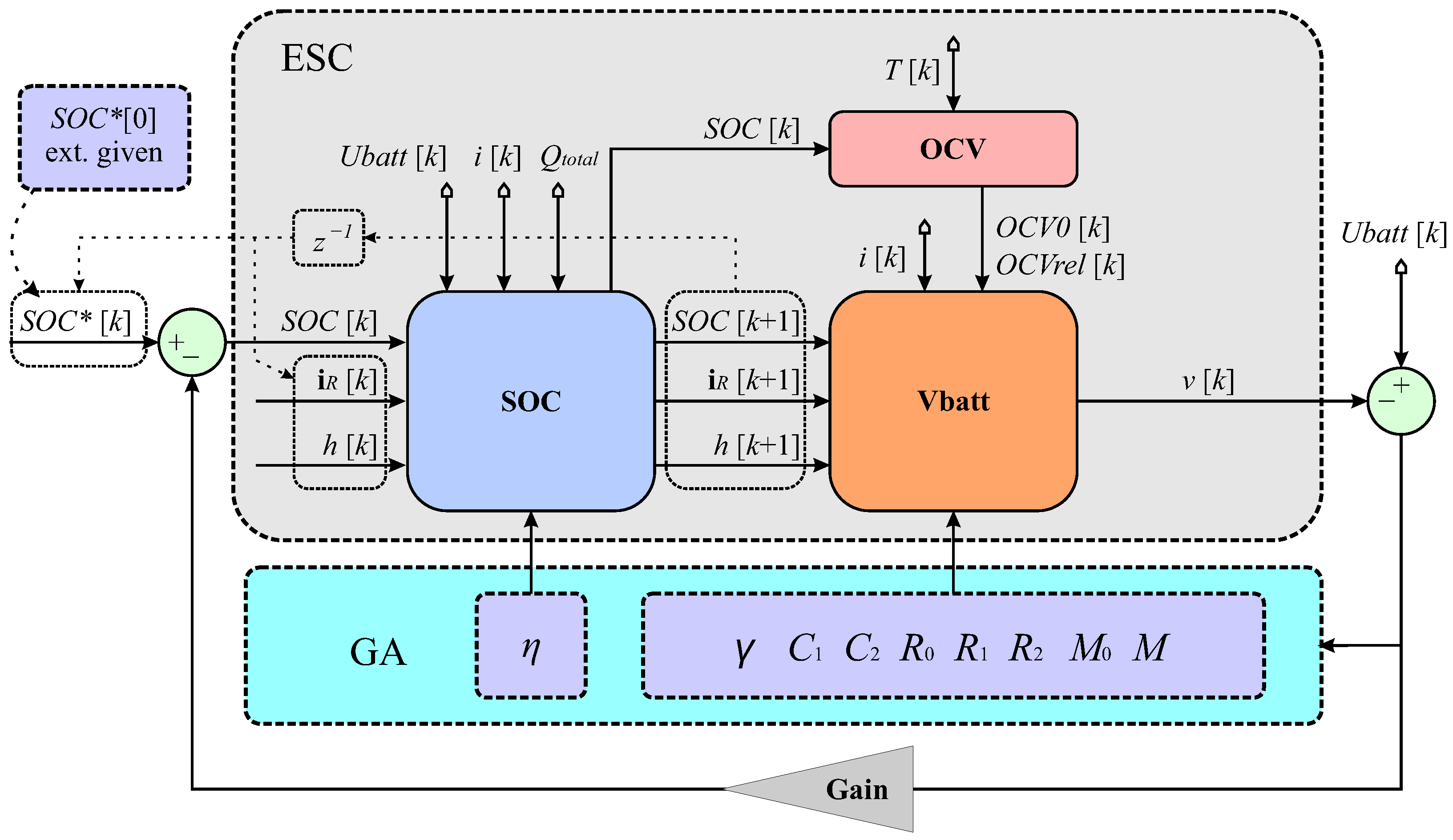
2.3.4. GA-ESC+FB: Initial SOC0 Set to Arbitrary Value and Corrected by FB, ESC Parameters Determined by GA

The GA-ESC+FB framework utilizes a modified ESC model with an additional feedback loop and $Gain$ parameter. The GA-ESC+FB tuning of ESC parameters is similar to the GA-ESC. A set of trial solutions is given to the ESC and the mean squared error using these ESC parameters on the underlying experimental training cycle is calculated. The lower the mean squared error, the better the fitness.

Again, the initial SOC0 (denoted as $SO{C}^{\ast }\left[0\right]$ in Figure 5) is given externally. However, this time the initial SOC0 can be externally given as an arbitrary number between 0% and 100%. There is no need to measure it, which is the benefit of using GA-ESC+FB compared to the GA-ESC. The feedback loop with the variable $Gain$ parameter then acts as a correction mechanism to correct the error between uncorrected $SO{C}^{\ast }\left[k\right]$ and actual $SOC\left[k\right]$ as follows. If $v\left[k\right]$ overreads the $Ubatt\left[k\right]$, the error $Ubatt\left[k\right]-v\left[k\right]$ becomes negative and the $SO{C}^{\ast }\left[k\right]$ is reduced. If $v\left[k\right]$ underreads the $Ubatt\left[k\right]$, the error $Ubatt\left[k\right]-v\left[k\right]$ becomes positive and the $SO{C}^{\ast }\left[k\right]$ is increased. Such correction does not take place in a single step, but rather gradually with time (we expect that the largest error will be at the beginning). The adaptation of the $Gain$ parameter controls allowed corrections. The equation that follows represents the feedback loop mechanism numerically.

$$\mathrm{SOC}\left[k\right]={\mathrm{SOC}}^{\ast }\left[k\right]-Gain\times (U_{\mathrm{batt}}\left[k\right]-v\left[k\right])$$

(12)

The advantage of GA-ESC+FB lies in the constant self-correcting action. While the GA is run once only to determine the proper ESC parameters during the GA training period, the FB mechanism is run constantly during the testing period (and also during the remaining life cycle of the battery cell) as well. Still, the FB is not able to compensate for diminishing SOH due to aging. To address the aging of the battery cell, new ESC model parameters should be recalculated recurrently every now and then (based on the underlying time period).

2.3.5. GA-(ESC+SOC0): ESC Parameter and Initial SOC0 Both Determined by GA

The GA-(ESC+SOC0) is similar to the GA-ESC method. The main difference between the two is that besides seeking the optimal ESC model parameters it seeks the initial condition of SOC0 as well. Practically this means that the dimension of the problem is incremented by +1. Figure 6 exhibits the GA-(ESC+SOC0) method.

GA-(ESC+SOC0) is a simple yet effective hack of the fundamental GA-ESC. Instead of realizing the initial condition SOC0 by hand, it is being found automatically during the ESC model parameters searching.

3. Experiments and Results

The goal of the experiments was twofold: (1) implement all proposed five SOC estimation methods (including the ECC and EKF) with real laboratory equipment, and (2) utilize all of these to estimate the SOC of a real battery cell and realize the main differences between the frameworks.

3.1. Laboratory Setup

Laboratory measurements of the battery cell consisted of current in the k-th time step $i\left[k\right]$, measured voltage $U_{batt}\left[k\right]$, and temperature $T\left[k\right]$, all depicted in Figure 2. The laboratory framework was connected to a personal computer (PC) to monitor the batteries in real time via a microcontroller (MCU). A processor-in-the-loop system, STM32 MCU, was deployed for two-way information transfer. The DC electronic load Rigol DL3021A acted as an (electronic) load, and the Rigol DP8921A served as a programmable DC power supply, i.e., the current source. Information regarding the best obtainable accuracy per unit of measurements for the given experimental system is described in

Table 2. Accuracy obtained and ranges of units of measurements of the data acquisition hardware, built on purpose.

Parameter	Value
Voltage measure accuracy of cell	±1.25 mV
Current measure accuracy of cell	±625 µA
Temperature measure accuracy of cell	±0.1 °C
Temperature measure accuracy of temperature chamber	±0.2 °C
Min. reachable temperature of temperature chamber	−15 °C
Max. reachable temperature of temperature chamber	+70 °C

.

Figure 7 depicts the hardware equipment utilized during the experimental tests. A battery cell measurement card was built purposely, with an integrative holder for a single battery cell. The measurement card supports many different types of battery chemistry. Figure 8 depicts the results obtained. The first subplot shows the OCV obtained at a given temperature, varying from $T_a=-5 °\mathrm{C}$ to $T_a=45 °\mathrm{C}$. The subplot below depicts the calculated temperature correction factor OCVrel.

The dependency on the steady-state ambient temperature $T_a$ was recorded experimentally using the temperature chamber. Due to the very low charging/discharging reference current, i.e., $i_{ref}=C/30$, the warming effect of the battery was neglected, which implied that the battery temperature T equaled the ambient temperature $T=T_a$. We cycled the battery and monitored the current and OCV. Next, the total capacity $Q_{total}$ was calculated by integrating current with time, for the discharging cycle at $T=25$ °C [1] (SOC here dropped from 100% to 0%). Conversion of the x-axis from capacity to SOC was conducted where the total capacity equaled an SOC of 100%. Next, the effect of internal resistance was carefully studied, which is the reason why the charging and discharging OCVs differ (the Coulombic efficiency states the ratio between the two). The charging cycle was rescaled to fit into the SOC 0–100% domain and the battery internal resistance (which on the diagram symbolically changes from 0 to 100%) was averaged across the complete SOC domain. Finally, the single OCV-SOC curve was plotted accounting for the single averaged battery internal resistance [1].

The complete dependency on steady state ambient temperature $T_a$ was recorded experimentally [1] by forcing the battery into different temperatures, ranging from $T_a=-5$ °C to $T_a=45$ °C with steps of $\Delta T=5 °\mathrm{C}$. For each temperature, the OCV-SOC curve was extracted. An interpolation of OCV-SOC with respect to SOC and temperature can be used in practice. Once this step was finished, two diagrams were extracted using matrix algebra [1]. First, the OCV0 diagram showed the relationship between OCV and SOC for $T_a=0$ °C. Second, the OCVrel diagram showed the relationship between the OCVrel compensation factor, given in $\mathrm{V}/°\mathrm{C}$, and SOC, given in percent. Typically, both are highly nonlinear functions, as depicted in Figure 8.

In the out-of-steady-state scenario where the battery undergoes a variable current profile, its temperature does not equal the ambient temperature $T\ne T_a$. The higher the current flowing, the higher the temperature due to the internal resistance (increasing the current warms the battery and hence the indication $T\left[k\right]$). The higher the ambient temperature, the higher the battery temperature. Fixing the $SOC\left[k\right]$ constant and ceteris paribus in a steady state condition gives the $OCVrel\left(SOC\right[k\left]\right)$ constant, further implying that the higher the battery temperature the higher the OCV, i.e., a linear relationship. However, if SOC is not constant, ceteris paribus, a non-linear relationship between OCVrel and SOC, exhibited in Figure 8, is established. The temperature correction factor $OCVrel$ varies with the function $OCVrel\left(\right)$. A complete steady-state OCV equation is derived by summing two independent terms, i.e., the OCV0 and the OCVrel. The OCV0 is conducted by interpolating the OCV curve, which is given in a tabular form and held constant in all cases. The OCVrel term gives the temperature correction by multiplying $T\left[k\right]·OCVrel\left(S0C\right[k\left]\right)$. For example, if the measured battery temperature is $20$ °C and the $SOC=10\%$, this gives $OCVrel(SOC=10\%)=-0.5e^{-3}\mathrm{V}/$°C from Figure 8, which further implies that $T\left[k\right]·OCVrel\left(S0C\left[k\right]\right)=20 °\mathrm{C}·(-0.5e^{-3}\mathrm{V}/°\mathrm{C})=-0.01$ V, a small negative correction factor for a given setting. The OCVrel compensation can be performed for the measured temperature range only, so a rough estimation of working temperatures needs to be conducted.

3.2. GA Setup and Estimation of ESC Model Parameters by GA

For optimization purposes, the elitism-enhanced GA was used; the experimental setup is outlined in

Table 3. GA setup. * = in case of GA-(ESC+SOC0) the $D=10$ due to the additional parameter of SOC being optimized. ** = $p_m$ is tunable and can gradually be increased to 1 if optimization is caught into the local optimum and immediately decreased to a minimum value of 0.0001 when the optimization is out of the local optimum. $f{f}_{min}$ is a fitness function value threshold that stops optimization once this value is hit.

Parameter	Symbol	Value
Population size	NP	200
Max. no. of generations	MAX_GEN	500
Fitness function threshold	$f{f}_{min}$	0.01
Binary chromosome length (genotype length)	$N_c$	16
Dimension of the problem	D	9 *
Elitism	E	2
Initial probability of mutation	$p_m$	0.0001 **
Probability of crossover	$p_c$	0.8
Objective		minimize

. Genetic operators included roulette wheel selection, single-point crossover, bit-flip mutation and elitism. Termination conditions were set as either the reached maximum number of generations, or the fitness function value threshold. The representation of individuals was binary. The probability of mutation was set to be adaptive, ranging from $p_m=0.0001$ to maximum $p_m=1$. The following rule has been applied to the adaptation of the probability of mutation $p_m$. The fitness function value averages $f{f}^{\left(avg\right)}$ were monitored for: (1) the last $g-6$ to $g-4$ generations $f{f}_{(g-6:g-4)}^{\left(avg\right)}$, (2) the last $g-3$ to $g-1$ generations $f{f}_{(g-3:g-1)}^{\left(avg\right)}$. All fitness function evaluations were included here. If the value $f{f}_{(g-3:g-1)}^{\left(avg\right)}$ remained bounded between positive and negative thresholds, as shown symbolically, then the probability of mutation increased by 1 percentage point, i.e., for $\Delta p_m=0.01$. Otherwise, the probability of mutation was reset to $p_m=0.0001$. This process was repeated indefinitely.

$$p_m=\left\{\begin{array}{cc}{p}_m+\Delta p_m\hfill & f{f}_{(g-3:g-1)}^{\left(avg\right)}\in \left[f{f}_{(g-6:g-4)}^{\left(avg\right)}\pm 0.2\right]\hfill \\ 0.0001\hfill & \mathrm{otherwise}\hfill \end{array}\right.$$

(13)

Effectively, this adaptation was implemented as a mechanism to prevent convergence into the local optima. It was realized experimentally that such adaptation increased the system identification success drastically. Algorithm 3 represents the pseudo-code of the GA utilized, where the $NP$ stands for population size (number of individuals).

The GA was utilized to tune the ESC model parameters, for which real battery data were necessary. An ESC model parameters experimental cycle, including charging and discharging profiles in the duration of almost 10 h, was utilized. The experimental cycle is depicted in Algorithm 4 (relaxing the battery means $i_{ref}=0$ A.). The tuning profile included periods of abrupt and rapid changes in load, as well as stationary periods. Moreover, these two periods were interchanged and repeated. Two such cycles, run one after the other, were run in order to estimate the ESC model parameters, as shown in Figure 9.

Algorithm 3 Elitist-Enhanced Genetic Algorithm

1: Initialize population $NP$ with random solutions   2: Evaluate the fitness of each individual in $NP$   3: while stopping criterion not met do   4:       Convert population $NP$ into binary form (genes)   5:       Select parents for reproduction   6:       Perform crossover and mutation to create offspring   7:       Convert binary genes of the population $NP$ back into a decimal representation   8:       Evaluate the fitness of the offspring   9:       Apply elitism: select the best individuals for the next generation 10:       Replace the worst individuals in the population with offspring 11:       Apply probability of mutation $p_m$ adaptation 12: end while

Algorithm 4 The experimental cycle to tune the ESC with GA as depicted in Figure 9

1: Initialize empty lists and monitor each time step: T, i, $Ubatt$, $i_{ref}$   2: for i = 1,2 do   3:       Relax for 30 s   4:       Discharge at $i_{ref}=1$ A for 5 min then relax for 5 min   5:       Discharge at $i_{ref}=3$ A for 5 min then relax for 5 min   6:       Discharge at $i_{ref}=5$ A for 30 s then relax for 5 min   7:       Charge at $i_{ref}=1$ A for 5 min then relax for 5 min   8:       Discharge at $i_{ref}=3$ A for 30 s   9:       Charge at $i_{ref}=1.5$ A for 30 s 10:       Discharge at $i_{ref}=3$ A for 30 s 11:       Charge at $i_{ref}=1$ A for 30 s then relax for 1 min 12:       Charge at $i_{ref}=0.5$ A for 5 min then relax for 30 s 13:       Discharge at $i_{ref}=2$ A for 1 min 14: end for 15: Output: T, i, $Ubatt$, $i_{ref}$ vectors

As seen from the figure, the discharging cycle introduced short charging bursts. These were introduced to help estimate more accurately the parameters of the ESC model, especially parameters of the RC links ($R_1$, $C_1$, $R_2$, $C_2$), which are supposed to define the temporal dynamics.

The GA was utilized to estimate the ESC model parameters. Ten different runs of the GA were held and the best run of these, according to the best fitness function value $f{f}^{\left(best\right)}$, was taken as a final solution. The fitness function value was calculated as follows:

$$\mathrm{ff}={\displaystyle \frac{1}{n}}·\sum _{k=0}^n{(U_{\mathrm{batt}}\left[k\right]-v\left[k\right])}^2$$

(14)

where n is the number of samples within the repeated experimental cycles.

Table 4. Best found ESC model parameters and appropriate best fitness function value, among the 10 independent runs of the GA. “up. lim.” = upper limit, “low. lim.” = lower limit.

	GA-ESC	GA-ESC+FB	GA-(ESC+SOC0)	Low. Lim.	Up. Lim.
$f{f}^{\left(best\right)}$	0.5484	0.5287	0.5394	n/a	n/a
$R_0[\Omega ]$	0.0208	0.0211	0.0275	0	0.2
$\eta$	1	1	0.9200	0.9	1
$\gamma$	59,432	17,126	15,171	0	60,000
M	0	0	0	0	0.1
$M_0$	0.0024	0.0015	0.0021	0	0.01
$R_1[\Omega ]$	0.0119	0.0259	0.0258	0	0.2
$C_1\left[F\right]$	1634	45,112	49,984	0	60,000
$R_2[\Omega ]$	0.0200	0.0156	0.0109	0	0.2
$C_2\left[F\right]$	27,037	1795	10,000	0	60,000

exhibits the best-found ESC model parameters by the GA, for each of the methods separately. The best-found ESC parameters by GA will not be unique as different combinations of parameters lead to the approximately same solutions. This is the main reason why such differences arise between multiple independent runs. Kalogiannis et al. [48] have empirically shown that the robustness of the found solutions may thus vary heavily.

The best found M was found to be zero in all three cases as follows: By increasing the $\gamma$, the term $A_H\left[k\right]\to 0$. Having that, the term $A_H\left[k\right]·h\left[k\right]\to 0$ and $(A_H\left[k\right]-1)\to -1$, which further means that $(A_H\left[k\right]-1)·sgn\left(i\left[k\right]\right)\to -sgn\left(i\left[k\right]\right)$. As this is exactly opposite to the instantaneous hysteresis voltage $s\left[k\right]$, the optimization algorithm eliminates this term by setting the $M=0$. As proposed methods are offline only, further adaptations of ESC parameters, accounting for changes in temperature or SOH, are not possible.

3.3. Experimental Setup and Conduct of Experiments

The experiment involved a recurrent experimental testing cycle that was repeated 20 times. Before the experimental testing, the battery was charged fully and then relaxed for 2 h at reference current $i_{ref}=0$ A. The ECC and EKF were benchmarks for estimating SOC with externally given initial conditions ($SOC0=100\%$). The three proposed models, i.e., GA-ESC, GA-ESC+FB and GA-(ESC+SOC0) involved a feedback loop FB with variable gain. The initial condition on SOC0 was thus not relevant for these three methods, as the FB guaranteed convergence towards an unbiased estimate of the SOC. Hence, the initial condition was set to be $SOC0=50\%$, as setting it to a middle ensured the lowest latency when converging to either extreme value, e.g., 100 or 0 %. Figure 10 depicts the ESC as was used during the experimental testing, i.e., exploitation. The three different sets of ESC parameters were tested (initial conditions on SOC0 were given externally and fixed to be $SO{C}^{\ast }\left[0\right]=50\%$).

The $Gain$ parameter was realized experimentally. By setting it to a high value of $Gain=0.1$ it was realized that the estimation bias was compensated rapidly. However, such a high value produced estimation instabilities in the range of SOC below 10% and above 90%. Therefore, a lower value of $Gain$ was selected for these two areas, as follows:

$$Gain=\left\{\begin{array}{cc}0.1,\hfill & \mathrm{if}10\%\le \mathrm{SOC}\left[k\right]\le 90\%\hfill \\ 0.0001,\hfill & \mathrm{otherwise}\hfill \end{array}\right.$$

(15)

The reference current profile was determined prior to conducting the experimental test. The reference current profile involved short charge and discharge bursts as well as steady-state periods of charge and discharge. It was set by a combination of electronic load and DC power supply. Algorithm 5 exhibits the reference current profile for a single testing cycle. Figure 11 exhibits the same experimental testing cycle graphically.

Algorithm 5 Recurrent experimental testing cycle as depicted in Figure 11

1: Initialize empty lists and monitor each time step: T, i, $Ubatt$, $i_{ref}$   2: for l do = 1, 2, 3, …, 20   3:       for m do = 1, 2   4:             Short discharge burst at $i_{ref}=1$ A for 10 s then relax for 10 s   5:             Short discharge burst at $i_{ref}=5$ A for 10 s then relax for 10 s   6:             Short discharge burst at $i_{ref}=10$ A for 10 s then relax for 10 s   7:             Short discharge burst at $i_{ref}=15$ A for 10 s then relax for 10 s   8:             Short discharge burst at $i_{ref}=20$ A for 10 s then relax for 10 s   9:             Steady-state discharge at $i_{ref}=1$ A for 5 min then relax for 1 min 10:             Short charge burst at $i_{ref}=1$ A for 10 s then relax for 10 s 11:             Short charge burst at $i_{ref}=2$ A for 10 s then relax for 10 s 12:             Short charge burst at $i_{ref}=3$ A for 10 s then relax for 10 s 13:             Short charge burst at $i_{ref}=4$ A for 10 s then relax for 10 s 14:             Short charge burst at $i_{ref}=5$ A for 10 s then relax for 10 s 15:             Steady-state discharge at $i_{ref}=5$ A for 1.67 min then charge at $i_{ref}=3$ A for 1.67 min 16:             Steady-state discharge at $i_{ref}=10$ A for 1.67 min then charge at $i_{ref}=5$ A for 1.67 min 17:             Steady-state discharge at $i_{ref}=5$ A for 1 min then charge at $i_{ref}=5$ A for 1 min 18:             Steady-state discharge at $i_{ref}=4$ A for 5 min then charge at $i_{ref}=4$ A for 5 min 19:             Relax for 10 s 20:             Steady-state discharge at $i_{ref}=1$ A for 5 min then charge at $i_{ref}=1$ A for 5 min 21:             Steady-state discharge at $i_{ref}=2$ A for 5 min then charge at $i_{ref}=2$ A for 5 min 22:             Steady-state discharge at $i_{ref}=3$ A for 5 min then charge at $i_{ref}=3$ A for 5 min 23:             Steady-state discharge at $i_{ref}=4$ A for 5 min then charge at $i_{ref}=4$ A for 5 min 24:             Steady-state discharge at $i_{ref}=5$ A for 5 min then charge at $i_{ref}=5$ A for 5 min 25:             Steady-state discharge at $i_{ref}=6$ A for 5 min then charge at $i_{ref}=6$ A for 5 min 26:             Short discharge burst at $i_{ref}=10$ A for 10 s then charge at $i_{ref}=6$ A for 10 s 27:             Steady-state discharge at $i_{ref}=8$ A for 1 min then relax for 2 min 28:       end for 29:       Charge the battery cell at $i_{ref}=1$ A till $Ubatt=2.8$ V 30:       Charge the battery cell at $i_{ref}=C/30$ till $Ubatt=2.8$ V 31: end for 32: End of recurrent experimental testing cycle 33: Output: T, i, $Ubatt$ vectors   ▹ If terminal voltage $Ubatt\left[k\right]<1.5$ V, the for loop for index m is break and charging takes place immediately. Remark: Relaxing the battery battery means $i_{ref}=0$ A.

3.4. Results

The quality of the methods proposed and the benchmarks were tested using the experimental test, which involved cycling the battery in a recurrent loop 20 times. A single cycle loop took a bit more than 4 h and a half in average, while a complete experimental test took 92 h. Each loop involved the battery undergoing the reference current for a given period of time, as introduced by the experimental testing cycle in Algorithm 5. Actual current, temperature and terminal voltage of the battery cell were monitored during this period to form a testing dataset. Implemented methods were run on this underlying testing dataset to estimate the SOC in each time step. The recalibrations and limitations at 100% or 0% were excluded for all methods. Results were presented fourfold, each in a separate subsection, First, a complete 92 h experimental testing was plotted. Next, detailed plots for the first and the last experimental testing cycles were attached. Finally, statistical analysis and an affordability study were provided.

3.4.1. Complete Experimental Test

Figure 12 represents experimental test results. The upper subplot represents the actual terminal and predicted voltages for each method; the lower subplot shows the estimated SOC.

Long-term drift with respect to time is observable from two methods, the ECC and EKF. The ECC underestimates the SOC while the EKF overestimates the SOC, as no recalibrations were performed when SOC equaled either 0 or 100%. Proposed ESC methods worked similarly to each other and exhibited a stable performance over the whole range. No major deviations from the expected SOC were observed. The next subsection presents the first testing cycle in detail.

3.4.2. Detailed View of the First (Initial) Experimental Cycle

Figure 13 represents results on the first cycle in detail. The ECC worked reliably as no deviations nor outliers were observed. The EKF performed best during the first half of the cycle. Later, a drift and possibly an offset evolved which caused the EKF to overestimate the actual SOC. Consequently, SOC estimations of more than 100% were indicated by EKF. Proposed frameworks involving GA-ESC, GA-ESC+FB, and GA-(ESC+SOC0) gave reasonable voltage and SOC estimations, although they all started biased from the $SO{C}^{\ast }\left[0\right]=50\%$. The rapid convergence of the SOC is clearly noticed. However, none of the implemented methods were able to capture the predicted voltage $v\left[k\right]$ well when the SOC was above 90% or below 10%. When the SOC was below 10% and discharging, the battery cell exposed significant non-linearity which caused the measured terminal voltage to fall abruptly when under load. When the SOC was above 90% and charging, the battery terminal voltage increased abruptly. Significant deviations were detected for all estimation algorithms, although the GA-ESC performed best in this case, followed by the GA-(ESC+SOC0) and the GA-ESC+FB.

Minor SOC estimation deviations between methods themselves were noted after concluding the first experimental cycle. Two highly non-linear regions regarding the terminal voltage $Ubatt$ (1) when SOC was below 10% and discharging, and (2) when the SOC was above 90% and charging, were detected. None of the three proposed methods was able to capture abrupt voltage changes $\Delta Ubatt$ within these two regions. Despite this fact, no drift accumulation when outside these two regions was detected, as the deviations were corrected soon when the new terminal voltage outside these two regions was established.

3.4.3. Detailed View of the Twentieth (Last) Experimental Cycle

Figure 14 shows detailed results on the last experimental cycle. The ECC strongly deviated from the proposed ESC methods. Its SOC estimations were prone to drifting with respect to time. With each cycle, the SOC estimations were underestimating the actual SOC more and more. After 10 cycles the ECC exhibited significantly negative SOC values. This was due to the fact that ECC rests on the traditional current integration.

On the other hand, the EKF and GA-ESC were consistently overestimating values of the SOC of more than 100%, but never more than 4 or 0.6 percentage points for EKF and GA-ESC, respectively. During experimental tests, the GA-(ESC+SOC0) never reached more than 99.5% and the GA-ESC+FB never reached more than 99%, when the battery was fully charged. This meant max. 1 percentage point of error for all three proposed methods which is a very solid performance.

3.4.4. Statistical Results and Affordability of the Proposed Frameworks

Table 5. The MSE (mean squared error) and MAE (mean absolute error) of the predicted voltage $v\left[k\right]$ for each method. Lower score represents better solution.

	MSE $[\times {10}^{-3}]$			MAE $[\times {10}^{-3}]$
Cycle	1st	20th	All	1st	20th	All
EKF	1.73	3.07	2.76	16.48	26.26	25.02
GA-ESC	2.09	2.86	2.58	23.88	25.79	24.86
GA-ESC+FB	2.54	3.67	3.33	29.50	32.93	32.39
GA-(ESC+SOC0)	2.15	3.05	2.80	26.12	28.92	28.47

represents statistical results of voltage prediction errors $Ubatt\left[k\right]-v\left[k\right]$ tabularly. The ECC algorithm was not involved here as it was unable to predict the voltage $v\left[k\right]$ (just the SOC). Columns are separated by MSE and MAE statistical indicators. Each indicator shows squared errors for the first, last and all cycles. Please note that the Table 5 does not represent any SOC statistical errors, but the terminal to predicted voltage $Ubatt\left[k\right]-v\left[k\right]$ errors only.

For the first cycle, differences in MSE and MAE between GA-ESC, GA-ESC+FB and GA-(ESC+SOC0) are negligible, but EKF works significantly better. The good performance of the EKF is partly due to the fact that EKF starts with proper SOC0 at the beginning, i.e., 100%, while proposed methods start at SOC0 equal to 50% and converge toward an unbiased estimate with time. As the process of converging takes time, large errors at the beginning are integrated that increase the MSE and MAE significantly. For the last cycle, the GA-ESC performs best for both MSE and MAE. The EKF is more competitive for the MAE than for MSE, which is an indicator of outliers presence. Namely, the MSE indicator is more susceptible to outliers than the MAE. The GA-ESC+FB performs worst for all cycle indicators. Please note that the table of SOC errors would be much more representative, instead of terminal voltage errors, but cannot be obtained as the true SOC is not known (exceptions apply for 2 points, SOC equal to 100 and 0%).

The affordability of the proposed frameworks comes in two parts. The first part represented obtaining the battery data utilizing the underlying experimental training cycle that lasted in our case 5680 s (which roughly equals to 1 h and 35 min). In this time, the battery was statically and dynamically excited within different time periods under different loads. Electronic load and auxiliary power supply were used to ensure accurate readings. During that time, battery cells were unable to perform any useful work, i.e., a serious drawback compared to online methods such as RLS. The second part represented the computational complexity of a GA for battery identification (the ESC model). Based on the recorded experimental cycle, the GA, on average spent $251.14\pm 1.23$ min ($N=10$), which roughly equaled 4 h and 11 min for GA-ESC and GA-ESC+FB (on a personal computer). For the GA-(ESC+SOC0) this process took even more time due to an additional dimension. Two facts need to be mentioned here. The first fact is that optimization was executed for a maximal number of generations ($MAX\_GEN=500$) without hitting the early-stopping criterion. Still, minor or no improvements were spotted after the $GEN=100$. By early-stopping at $GEN=100$ the execution time would decrease by a factor of 5, which is less than 1 h, and the quality of results would not have been hurt much. The second fact is that the used programming code for the GA was written in an interpreter programming language and little effort was put into its optimization. Further optimization of programming code and transfer to a compiler programming language would significantly decrease computational complexity. Also, a graphical process unit could be used for a parallel calculation of a GA, especially the fitness function evaluation which took most of the time.

Theoretically, there is no need to run the GA on the dedicated hardware as this can be run offline on the computer server. Still, experiments have been made on a dedicated digital signal processor with minimal resources but highly optimized programming code, which revealed that the GA identification can finish in less than a minute. This is not such a drawback compared to the online RLS, since the GA can be implemented similarly to the online RLS. For example, in each time step a single GA generation can be executed and by incrementing the time steps, better and better solutions are found. Then, a real-time parameter adaptation by GA is possible by monitoring the data within the moving window. Still, the initial dataset experimental cycle needs to be prerecorded as GA may not converge if the experimental cycle too short.

4. Discussion

Three different underlying designs for predicting the state-of-charge given its uncertain initial conditions were implemented and tested. The simplest of all was the direct method called enhanced Coulomb counter which was only able to predict SOC without estimating the state space vector. Two other designs, the extended Kalman filter and enhanced self-correcting mechanism, optimized by a genetic algorithm, estimated the state space vector too. Given appropriate settings, both of these designs should have ensured unbiased estimates of the state of charge of a lithium-ion battery cell.

The enhanced Coulomb counter functioned as expected. In the short term, it was seen as a reliable indicator. In the long term, integral drift with respect to time prevented it from making unbiased estimates. Soon after the last recalibration at a state-of-charge equal to 100%, it began predicting a negative state-of-charge. The extended Kalman filter performed with more stability. Minimal bias, possibly an offset, was spotted in the long term and caused the Kalman filter to overread the actual state-of-charge by approximately four percentage points. Further analysis would be necessary to determine the exact cause.

One of the proposed frameworks, i.e., the enhanced self-correction model with a feedback loop, seemed the best option. The variable $Gain$ of the feedback loop tends to control the convergence rate to the unbiased estimate of state-of-charge. Some experiments were necessary to properly determine the $Gain$ parameter, if set to high it may have caused instabilities; if set to low, the convergence rate was slow. This framework functioned well even if an arbitrary value of the state-of-charge initial condition was input. The other two alternatives of the enhanced self-correcting model without the feedback loop needed prior knowledge of the state-of-charge initial condition.

In the future, it would be crucial to address the changing battery parameters due to aging. Keeping the identified model constant may induce bias in state-of-charge predictions. Battery parameters are not obliged to be updated continuously, as there is no need for this, but they should be updated every now and then at underlying update times. These update times may be either (1) fixed, for example, after five discharging/charging cycles, or (2) adaptive after the battery cell was misused due to over-charging/-discharging or discharging with too high currents, etc. A time window with all the necessary data needs to be recorded and a “silent” genetic algorithm execution, where in each time step only a single generation is executed (or even less) to prevent non-real-time microcontroller behavior, would need to be implemented.