Continuous Flow Labeling and In-Line Magnetic Separation of Cells

Abstract

There is an identified need for point-of-care diagnostic systems for detecting and counting specific rare types of circulating cells in blood. By adequately labeling such cells with immunomagnetic beads and quantum dots, they can be efficiently collected magnetically for quantification using fluorescence methods. Automation of this process requires adequate mixing of the labeling materials with blood samples. A static mixing device can be employed to improve cell labeling efficiency and eliminate error-prone laboratory operations. Computational fluid dynamics (CFD) were utilized to simulate the flow of a labeling-materials/blood mixture through a 20-stage in-line static mixer of the interfacial-surface-generator type. Optimal fluid mixing conditions were identified and tested in a magnetic bead/tumor cell model, and it was found that labeled cells could be produced at 1.0 mL/min flow rate and fed directly into an in-line magnetic trap. The trap design consists of a dual flow channel with three bends and a permanent magnet positioned at the outer curve of each bend. The capture of labeled cells in the device was simulated using CFD, finite-element analysis and magnetophoretic mobility distributions of labeled cells. Testing with cultured CRL14777 human melanoma cells labeled with anti-CD146 1.5 μm diameter beads indicated that 90 ± 10% are captured at the first stage, and these cells can be captured when present in whole blood. Both in-line devices were demonstrated to function separately and together as predicted.

1. Introduction

Effective rare-target-cell capture and detection methods have been proven (reviewed by Labib, 2021 [1]) and commercialized, including the CellSearch platform [2], the only one approved by FDA to date for the enumeration of circulating tumor cells. This and most methods of rare cell enrichment utilize immunomagnetic labeling and magnetic capture of target cells; however, a number of microfluidic platforms capture target cells on antibody coated surfaces, while others rely on non-specific separations based on fluid dynamics. In all cases, workflow simplification and improved efficiency of capture are seen as persisting goals [1]. Continued research is required to develop a reliable point-of-care (POC) system for target-cell detection in large blood samples. Several microfluidic systems exist that require the pre- or post-processing of samples, or are unable to accommodate the several (up to 25) mL of blood sample [1,3,4,5] required for adequate statistical sampling. The combined automation of cell labeling and collection not only supports POC diagnostics, but also speeds workflow and increases throughput, whether in the laboratory or at POC. Target cell labeling without centrifugation steps and proven methods for cell capture need to be combined with a well-designed channel (trap), and collected cells need to be easily transferred from the trap to a detector for detection/quantification. Simulating the flow of labeled cells through a labeling device and capture device is critical to confirm the efficacy and speed of the entire system; similar simulations have been performed on POC devices for other cells/materials [6,7,8]. Cell labeling, collection, detection and quantification all must work in unison for an effective, user-friendly POC device. In this study, we establish parameters for optimized automated capture of rare target cells from up to 25 mL of whole blood. Although the sensitivity available in existing rare-cell detection procedures [2,9] was not matched, the results of this study affirm that target cell collection can be automated to the extent that it can be performed by semi-skilled point-of-care operators.

2. Materials and Methods

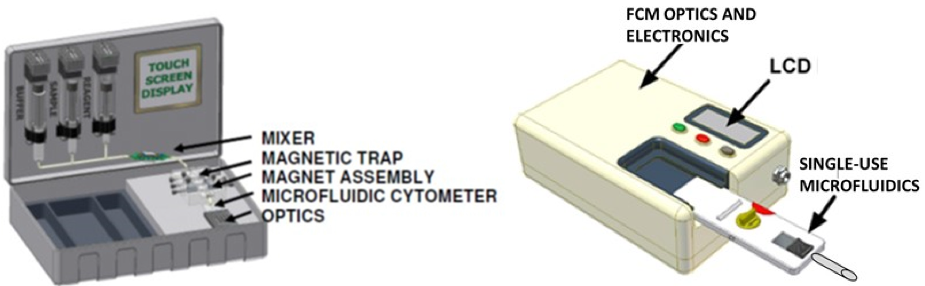
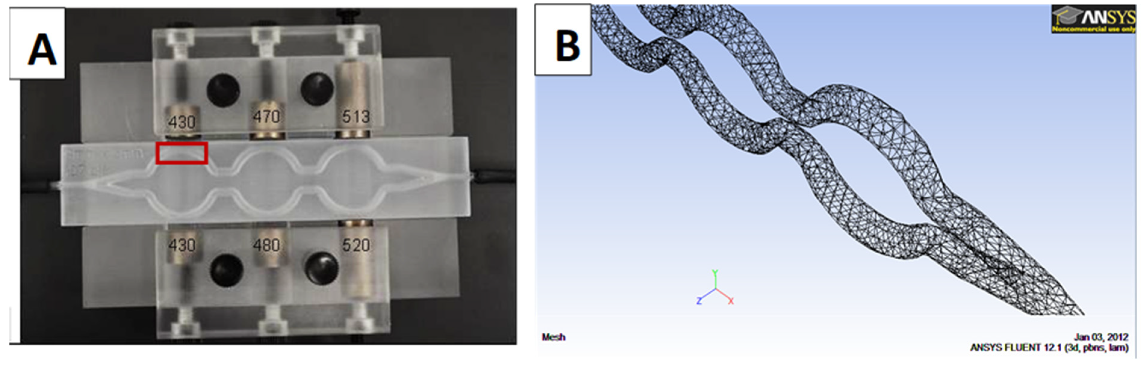
2.1. In-Line Mixing Device

Figure 1A shows the static mixer with a tube diameter of 1 cm and a tube length of 15 cm. The mixer has 20 helical baffles that divide the fluid mixture into multiple layers. Figure 1B illustrates how this is accomplished.

The static mixer is considered an Interfacial Surface Generator (ISG) with no moving parts [10]. In-line mixers have found their way into microfluidic processors, including a patented processor for magnetically labeled cells for microfluidic flow cytometry [4,11]. The shape of baffles is designed for delivering two streams of fluids into the static mixer via a “T” joint. The helical shape is a widely used design for fluid division; flow over the baffles provides continuous mixing of a pair of fluids. At each new baffle, the fluid is divided into two layers. The result is an exponential increase in fluid stratification; Figure 1B shows the division of fluid flow. The number of striations produced is equal to 2ⁿ, where n is the number of baffles. Two important factors in setting the flow conditions for this mixer are particle diffusion and particle sedimentation. A Brownian motion is assumed for all particles in the flow stream, and the time to cross the striation is considered to be the diffusion time. The mixer is fed by a pair of precision syringe pumps (Cole-Parmer ew-74900-15), with settings adjusted according to the disposable syringe type used.

2.2. Cells and Labels

Two cultured tumor cell lines were used in this research. In labeling experiments testing the in-line mixer and magnetic trap, the tumor cell line used was CRL-211, DT40 chicken lymphoma (produced by American Type Culture Collection (ATCC)). The antibody used is mouse monoclonal M-1 Anti-Chicken IgM mu chain (Biotin) (produced by Abcam^TM). The components of cell culture media include 74% Dulbecco’s modified eagle’s medium (DMEM), 10% tryptose phosphate broth solution, 5% chicken serum and 1% ABAM (Antibiotic-Antimycotic mixture), all purchased from SIGMA^TM, and 10% fetal bovine serum (FBS) produced by ATCC^TM. Magnetic beads used in the testing were Dynabeads^® Biotin Binder (InVitrogen/Dynal), and the magnetic beads’ magnetophoretic mobility range was 1.3 to 2.0 × 10⁻¹¹ m³/TAs, while the concentration of beads was 4 × 10⁸ beads/mL and the concentration of tumor cells in phosphate-buffered saline was 1 × 10⁴ cells/mL. Cole-Parmer^TM ew-74900-15 syringe pumps were used. Cell samples were diluted to approximately 10⁵ cells/mL. The magnetic beads were first labelled by antibodies, then diluted to around 10⁷ beads/mL. For the mixing test, 8.3 mL of cell sample and 1.7 mL of reagent was pumped through the mixer in 10 min. As a comparative test, 8.3 mL of cell culture and 1.7 mL of reagent with same concentrations were combined in a test tube, and incubated on a rocker table for 30 min at a repetition rate of 15 rpm. After mixing, 1 mL of each sample was analyzed using the magnetic velocimeter (see Section 2.3).

The A2058 (ATCCCRL 11147) human melanoma cells used in labeling and trapping experiments were obtained from American Type Culture Collection and cultivated by serial transfer, and used in experiments immediately or stockpiled by slow freezing and storage at −80 °C. Magnetized tumor cells were produced for the capture tests as follows: CRL11147 cells were harvested from culture with a viability of >90%. These were centrifuged at 200× g for 10 min, re-suspended in 1 mL Dulbecco’s Phosphate Buffered Saline (PBS) and blocking buffer (6% bovine serum albumin—BSA) for 5 min, again centrifuged at 200× g for 10 min and re-suspended in 500 µL PBS. To this suspension was added 10 µL of the primary antibody Anti-MCAM, clone P1H12 (Millipore Sigma, Burlington, MA, USA) and incubated at 4 °C for 20 min. After addition of 10 mL PBS, the cells were centrifuged at 200× g for 10 min and re-suspended in 500 µL PBS, and secondary antibody (100 µL 1.5 µm diameter Biomag^TM beads coated with Goat anti-mouse IgG) was added and incubated at 4 °C for 20 min. These cells were fixed by adding 500 µL of Cyto-Chex, (Streck Innovations, Inc., Omaha, NE, USA) and incubated for 2 h before using in magnetic separation experiments or refrigeration for storage. They were diluted to a final feed concentration of 10⁴ cells/mL in PBS.

Bovine whole blood (Animal Tech, Tyler, TX, USA) or human whole blood (collected in compliance with Purdue University Internal Review Board into a standard Becton-Dickinson Vacutainer with 3.2% sodium citrate) was premixed with tumor sample and the antibody-labeled magnetic beads. Next, reagents and cells were combined in orbital or rocker-table mixing or within the in-line static mixer, and then fed into the magnetic trap.

2.3. Magnetic Reagents

3.27 μm diameter polystyrene beads with 14% iron oxide (Seradyn Thermo Fisher tsMGCM) were used as test particles for the magnetic trap. The magnetophoretic mobility µ_m was 7.47 × 10⁻¹² m³/TAs. These beads were diluted to 4.6 × 10⁸ beads/mL to make a concentrated feed for testing.

An indirect labelling scheme was used for magnetic human melanoma cell capture. 1.5 µm-diameter Biomag^TM beads coated with goat anti-mouse IgG1 from Bangs Laboratories (Cat. No. BM549) were used to bind with mouse P1H12 antibody that in turn recognized and bound to cells labeled with a mouse monoclonal anti-human CD146 antibody, a known human melanoma cell biomarker. The single-bead mobility is 3.70 × 10⁻¹² m³/TAs. Based on calculations the magnetophoretic mobility of a cell carrying 10 beads would be 5.5 × 10⁻¹² m³/TAs and one cell carrying 1 bead would be 0.5 × 10⁻¹² m³/TAs. The magnets must be able to capture cells within this mobility range. The magnetic labeling efficiency, under the reaction conditions used, was 90%. Magnetophoretic mobilities were measured using a magnetic particle tracking velocimeter (Hyperflux^TM, Magnaquant LLC, Louisville, KY, USA).

2.4. Properties of Components in the Simulated Labeling Mixture

The purpose of the mixer is to combine a 25 mL of whole blood sample consisting of red blood cells, white blood cells and target (in this case tumor) cells, as well as a 5 mL reagent solution consisting of immunomagnetic beads and antibody conjugated quantum dots. The mixture will flow through the tube at a flow rate of 1 mL/min (30 min for completion).

Table 1. Properties of cells, particles and quantum dots used in simulations.

Component	Diameter, µm	Density, g/cm3	Concentration, mL−1	Adheres to
Red blood cell	8.0	1.09	2 × 109	Nothing
White blood cell	10.0	1.07	2 × 106	Nothing
Target cell	10.0	1.07	100	MP and QD
Magnetic Particle (MP)	2.8	1.6	106	Target cell
Quantum Dot (QD)	0.02	2.0	107	Target cell

lists properties of cells, particles and quantum dots used in the calculations; concentration of target cells is low (usually less than the arbitrarily chosen 100/mL shown) when compared with the concentrations of the red (RBC) and white blood cells (WBC).

2.5. Magnetophoretic Mobillity Measurement

Magnetophoretic mobilities of cells and beads were measured using a Hyperflux^TM velocimeter (Magnaquant LLC), a particle analyzer/velocimeter that is used to measure the velocity of cells and particles based on their magnetophoretic mobility [12,13]. Motion is driven by a calibrated isodynamic magnetic field. Image sets created by a high-definition video camera are stored in memory, and can be used for processing and data evaluation. These image sets were captured using the IKOVision^TM program with specifically selected intensity threshold and size ranges [12]. Several particle parameters, including size, are recorded in a list-mode spreadsheet for detailed analysis by the user, using Microsoft Excel, for example. Composite images showing the tracks of moving particles over a period of 2 s (60 frames) are displayed, and magnetophoretic mobility histograms are calculated and displayed, and available as screen shots. The SI units of magnetophoretic mobility (velocity divided by ponderomotive force) are meters/second per Tesla-Ampere/meter² or m³/TAs [14].

2.6. Magnetic Trap

Figure 2 illustrates A: the magnet trap and B: the mesh file set for simulation. The version of the trap used in these studies was designed with three pairs of curved trapping stations and three pairs of magnets with pole-face field strengths of 430, 470 and 520 mT. At each station, the north pole of the magnet was adjacent to the channel. Thus, magnets of each pair, though at some distance from one another, were matched in north-to-north configuration to maintain maximum field divergence. The single-use channel assembly is produced by additive manufacturing and is removed from the magnetic fields for the collection of captured cells.

The two-channel, triple-trap design (1) assures the capture of all cells above a certain mobility, including those that are missed by the first stage or two of the trap due to broad mobility distributions and distance from the magnet(s); (2) allows the magnets to be close to the target cells due to the narrow channels; (3) accommodates channel cartridges with various channel geometries (narrow vs. wide); (4) accommodates a wide range of input volumes from 1 mL to an indefinite number of liters but especially the 30 mL sample volume anticipated in rare cell collection; and (5) provides a possibility of separately capturing and distinguishing two or three subpopulations of cells with different magnetic loads.

2.7. Fluorescence and Flow Cytometry

Antibody P1H12 reacts specifically with CD146 (MCAM, MUC18). Therefore, this primary antibody was reacted with the A2058 (ATCCCRL 11147) cells, and subsequently with Qdot^® 605 goat F (ab’) 2 anti-mouse IgG conjugate (H + L) Millipore Catalog # Q-11001MP. Fluorescence was analyzed using a Coulter “Quanta” cytometer and measuring red fluorescence using the FL3 signal.

3. Theory and Calculations

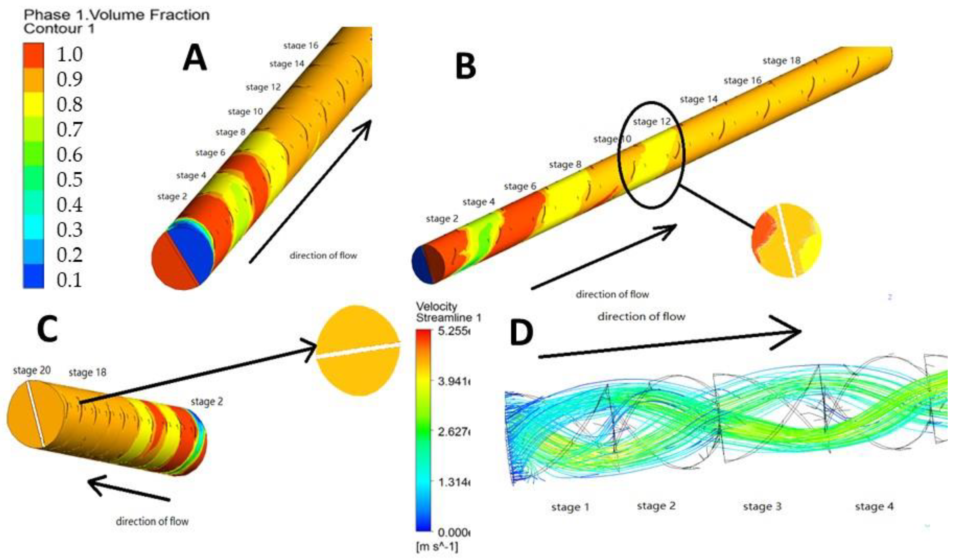
3.1. In-Line Mixer Simulations Using FLUENT^®

Using the ANSYS software, a mesh file was prepared and a model was used to simulate the flow development through the mixer. The model is set up in an ANSYS^tm ICEM CFD program. Based on the model, a laminar flow pattern was created for flow parameter calculation. To simulate the separation process more accurately, the simulation includes several factors including the multiphase mixing and the gravity effect on particles with respect to the motion of blood and reagent (particle suspension) within the system. Considering the number of inert blood cells, the effect of hindered flow within the system is considered. In the simulation a discrete model calculates the flow pattern of the blood cells, the magnetic particles and the quantum dots along with the interdiffusion of the two liquids. Results of the simulations will be able to direct the optimization of flow rates through the mixer. The dimensions of the mixer and the total flow rate requirement of 1 mL/min were used as inputs to determine: (1) the fraction of the phases at each stage of the mixer; (2) the stage of the mixer at which mixing could be considered complete based on the diffusion of the reactants; (3) entering streamline velocities; and (4) full-length streamline velocities.

3.2. Diffusion of Particles and Cells in the Mixer

The inlet fluids, consisting of blood and reagent, are considered as two phases. The baffles inside the mixer divide fluid into multiple layers, causing the particles and quantum dots to diffuse between phases. For well-mixed fluid, the particles need to travel the distance W between interfaces, which will be:

W = Rn⁻²

(1)

Here, R is the interior radius of the mixer and n is the number of stages; these factors can be used to calculate an estimated time for particles and quantum dots to diffuse by Brownian motion across the interfacial distance W. This diffusion time then must be applied to the remainder of the total operation time. By comparing the time needed for a particle to travel distance W and the time it stays inside the mixer, it is possible to determine whether the two phases can be well mixed. The Stokes-Einstein equation is used to calculate the time for diffusion

$$W=\sqrt{2Dt}$$

(2)

where W is the interfacial distance, t is the diffusion time and D is the diffusion coefficient, which is defined as

$$D=\frac{kT}{6\pi \eta a}$$

(3)

where k is Boltzmann’s constant = 1.38 × 10⁻²³ m² kg s⁻² K⁻¹, T is temperature, η is the fluid viscosity and a is the radius of a spherical particle. At T = 300 K (27 °C), fluid viscosity is assumed to be equal to the weighted average value of blood and reagent viscosities, or 3.5 cP = 0.0035 kgm⁻¹ s⁻¹. It may be assumed that the dissociation constant for the particle-cell reaction is zero, therefore the magnetic particles and quantum dots will instantly attach to a target cell when they come into contact.

3.3. The Effect of Sedimentation on Mixing

At low flow rates, gravity effects can cause sedimentation of blood cells and target cells, which can lead to unlabeled target cells. Sedimentation can also impede fluid flow through the mixer; understanding sedimentation rates for particles and cells is critical for optimum target cell labeling. Assuming the environment has no other disturbance and the particles are only affected by gravity, its sedimentation velocity v, according to Stokes law, is given by a balance of the drag force and the buoyant settling force, so that:

$$v=\frac{2a^2\left(\rho -{\rho }_0\right)g}{9\eta }$$

(4)

Here a is radius of the particle, $\rho$ and ${\rho }_0$ are densities of the particle and fluid, respectively, and g is the acceleration due to gravity, 9.8 m s⁻².

The Reynolds number Re of a single sedimenting particle is:

$$Re=\frac{2av\rho }{\eta }$$

(5)

The resistance force within the fluid also depends on the presence of other particles. With a higher volume fraction of particles, the flow between particles will have steeper velocity gradients and increased shear stresses.

The relationship between sedimentation rate and volume fraction can be determined experimentally, with a linear relationship between $\log v_c$ and $\log \left(1-\varnothing \right)$. The velocity of sedimentation should be adjusted as

$$v_c=v{\left(1-\varnothing \right)}^n$$

(6)

where v_c is the adjusted sedimentation velocity of particles in the mixing system, v is the sedimentation velocity of individual particles (Equation (4)), $\mathsf{\varnothing }$ is volume fraction of all of the particles in the suspension and n is a function of shape and Reynolds number [15].

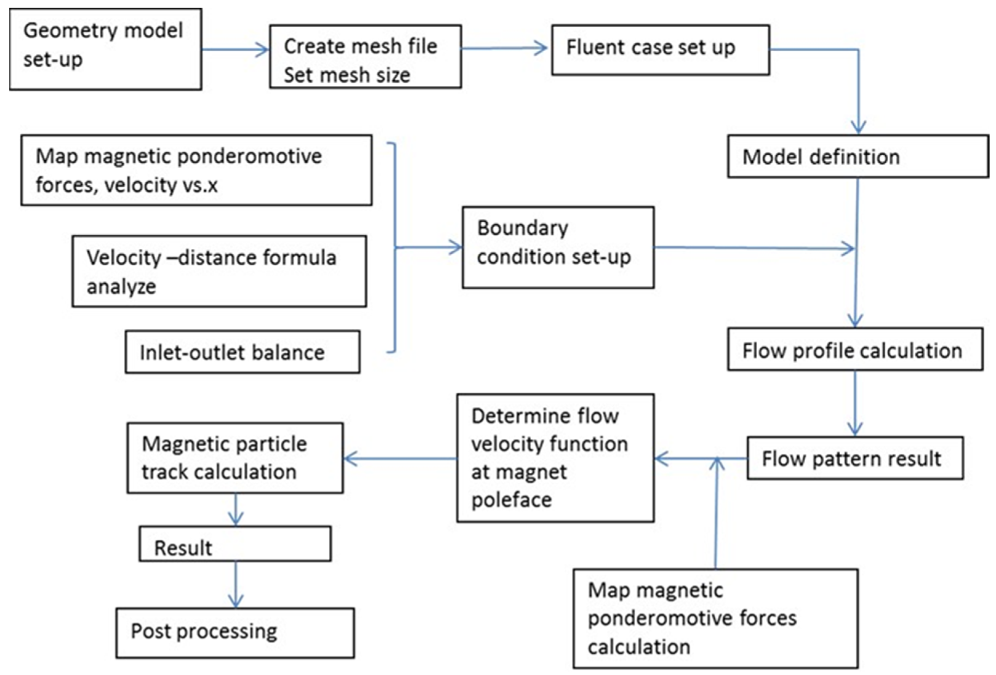
3.4. Magnetic Trap Simulations

Computational fluid dynamic analysis of the channel design was accomplished using the FLUENT^® analysis package, which performs the modeling of fluid flow and tracking particle movement in complex geometries. With the help of ICEM CFD^TM, a mesh file of the channel geometry was developed (Figure 2B) and a laminar flow model was employed for calculation. For the simulation of magnetic particles, the channel was simplified to a 2-D rectangle shape. A discrete model was applied to simulate the particle movement. The tracking of particles’ movement was performed to show the particle trapping efficiency. A flow chart, shown in Figure 3, summarizes the sequence for performing these operations.

The trajectories of magnetic particles were simulated by choosing a set of coordinates within the channel and adding the flow and magnetophoretic velocity vectors as a function of position in the mesh. At each step in time, the velocity is recalculated to account for simultaneous changes in streamline velocity, dy/dt, and magnetophoretic velocity, dx/dt.

3.5. Calculation of Particle Movement toward Magnets

To calculate the trajectory of a magnetic particle passing through the channel in a plane perpendicular to the pole piece, we calculate the flow velocity v_y of a massless particle using the CFD results and the magnetophoretic velocity v_x from the ponderomotive force. The magnetically induced ponderomotive force is given by

v_x = μ_m(B∙▽B)/μ_o

(7)

where v_x (m/s) is the velocity of particles towards the magnet pole face (in the negative x direction), µ_m is the magnetophoretic mobility and µ₀ is the permeability of free space with a constant of 1.257 × 10⁻⁶ Tm/A. µ_m varies based on the properties of magnetic particles. For the 3.27 µm-diameter magnetic beads, µ_m = 7.47 × 10⁻¹² m³/TAs, and for 1.5 μm-diameter beads used for labeling the CRL14777 melanoma cells, µ_m = 3.7 × 10⁻¹² m³/TAs.

4. Results and Discussion

4.1. Results of Static Mixer Simulation

4.1.1. Evaluation of Mixing of Input Fluids

Flow computations using the mesh shown in Figure 2B determined that Reynolds number throughout the mixer was below 200, meaning that laminar flow can be assumed. The ANSYS^tm FLUENT simulations of a total flow rate of 1.0 mL/min indicate a well-mixed stream at the center of the mixer, as illustrated in Figure 4A–C. The figure shows distributions of each phase according to volume fraction. Phase 1 is the blood sample (red) entering the mixer at 0.833 mL/min, and phase 2 is reagent (particle solution) (blue) entering the mixer at 0.167 mL/min. According to Figure 4A, after 11–12 stages of mixing, the volume fraction of the mixture reaches a balanced 83/17 ratio of blood volume to reagent volume. Figure 4B shows the middle stage of the mixer with the distribution of volume fraction in the cross section, indicating that mixing is not yet complete. Figure 4C shows that the blood and reagent are well mixed by stage 18 and at the outlet. Another set of simulations (Figure 4D) illustrates the streamlines of the particle velocities in the mixer. The difference between phase velocities was eliminated after 2–3 stages of mixing. Beyond stage 16, streamline velocities are very similar, at about 2.6 cm/s. Thus, static mixing succeeds in bringing reagents and blood to being fully mixed at the specified 1.0 mL/min flow rate.

4.1.2. Evaluation of Particle Diffusion and Collision in the Static Mixer

For each stage of the mixer, the layer width W was calculated (Equation (1)) and the time required for particles to diffuse this distance was computed (Equation (2)). The results in

Table 2. Calculated layer width in mm and diffusion times in seconds for quantum dots t (qdot) and magnetic particles t (mag particle) as a function of mixer stage number.

n (Stage)	W (mm)	t (qdot)	t (Mag Particle)
1.00	2.5	4.98 × 105	6.98 × 107
2.00	1.25	1.24 × 104	1.74 × 107
3.00	0.625	3.11 × 104	4.36 × 106
4.00	0.312	7.78 × 103	1.09 × 106
5.00	0.156	1.94 × 103	2.72 × 105
6.00	0.0781	486	6.81 × 104
7.00	0.039	121	1.70 × 104
8.00	0.0195	30.4	4.26 × 103
9.00	9.77 × 10−3	7.59	1.06 × 103
10.00	4.88 × 10−3	1.90	266
11.00	2.44 × 10−3	0.475	66.5
12.00	1.22 × 10−3	0.119	16.6
13.00	6.10 × 10−4	0.0297	4.16
14.00	3.05 × 10−4	7.41 × 10−3	1.04
15.00	1.53 × 10−4	1.85 × 10−3	0.260
16.00	7.63 × 10−5	4.63 × 10−4	0.0650
17.00	3.81 × 10−5	1.16 × 10−4	0.0162
18.00	1.91 × 10−5	2.90 × 10−5	4.06 × 10−3
19.00	9.54 × 10−6	7.24 × 10−6	1.02 × 10−3
20.00	4.77 × 10−6	1.81 × 10−6	2.54 × 10−4

show that for a 20-stage mixer, the quantum dots’ diffusion time beyond stage 10 is less than 0.5 min. The volume of the mixer is 12 cm³, so the time for the mixture to travel through the mixer is roughly 20 min at 1.0 mL/min. From these results, the static mixer provides enough time for particles to become well-mixed.

The flow rate of the blood sample is 0.83 mL/min and the flow rate of reagent is 0.17 mL/min. Considering information for cell types shown in Table 1, we can perform further analysis on the probability of interaction between cells, particles and quantum dots. For target cells, the concentration is about 83 cells/mL; and for magnetic beads, the concentration is about 1.6 × 10⁵ beads/mL, which means on average a magnetic bead will occupy 1/(1.6 × 10⁵) = 6.25 × 10⁻⁶ mL/bead, or 6.25 × 10⁶ µm³ per bead. Assuming that the shape of occupied space is cubic, the size of the cube is 184 by 184 by 184 µm, with the particle assumed to be the mass point at the center. To simplify the calculation, here we consider reagents and samples as well-mixed and magnetic beads having a uniform distribution. The length of this cube is much larger than a target cell (diameter = 10 µm), indicating a required diffusion distance for target/particle or target/quantum dot collisions. In the static mixer, the divided layer W is thinning with increasing stages. From the data in Table 2, when n > 5, the layer thickness W is less than the average distance between magnetic beads, indicating an increase in particle concentration within the cubic volume. When n > 9, the layer thickness W will be less than a target cell diameter, further increasing the likelihood of collision between magnetic beads and target cells.

Three processes influence the probability of collision between cells and magnetic particles: diffusion of magnetic beads; sedimentation of magnetic beads; and sedimentation of target cells. Given the cell diameter of 10 µm and the data of Figure 4, every cell is within about 80 µm of a magnetic bead. The times required to travel that distance by each of these processes, determined using Equations (2) and (4) are 10⁴ s for the diffusion of magnetic beads, 260 s for the sedimentation of magnetic beads and 80 s for the sedimentation of cells. Thus, the occupied area per bead ensures that they can reach target cells in the mixer. In conclusion, the calculation shows that magnetic beads will have a significant opportunity for collision with target cells. When considering the labeling process as a zero-order reaction, the cells are successfully labeled.

4.1.3. Calculation of the Effects of Sedimentation

It is necessary to ascertain that labeled target cells will not sediment to the lower surface of the mixer before they exit the mixer outlet. WBCs, target cells, magnetic particles and quantum dots are all assumed to be spherical, while the RBCs are assumed, for CFD purposes, to be cylindrical, with a height of 1.5$\mathsf{\mu }\mathrm{m}$ and a diameter of 10 $\mathsf{\mu }\mathrm{m}$. Diameters for magnetic particles and quantum dots are 2.8 $\mathsf{\mu }\mathrm{m}$ and 0.02 $\mathsf{\mu }\mathrm{m},$ respectively (Table 1). Taking the relative size into account and ignoring antibody arrangement on surfaces, the surface area of a target cell and a magnetic particle is roughly 314.16 µm² and 24.63 µm², respectively. We can thus simplify the model by assuming 10 magnetic particles and 100 quantum dots attached on one target cell. From the data in the tables, the labeled target cell’s overall volume is 6.38 × 10⁻⁷ mm³, the overall mass is 7.44 × 10⁻¹⁰ g and the average density is 1.16 g/cm³. Assuming the labeled cell’s shape is spherical, the average radius is 5.3 × 10⁻³ mm and the particle’s mass flow rate is 2.06 × 10⁻¹³ kg/s. The viscosity of fluid is close to blood, and thus it is considered as no higher than 0.035 g cm⁻¹ s⁻¹. Therefore, by using Equation (4), we obtain a sedimentation velocity v of an individual cell equal to 0.001 mm/s. Sedimentation velocity v is then used to calculate the Reynolds number (Re), which equals 0.0008 (Equation (5)). From experimental data [15], when Re < 0.2, corresponding to conditions under which inertial forces can be neglected, the exponent in Equation (6) is given by $n=4.65+\frac{19.5 d}{D}$, where d is diameter of particle and D is diameter of the static mixer. For labeled cells, the ratio d/D is essentially 0, so the result can be simplified to n = 4.65. The volume occupied by all particles in 1 mL is roughly 319 mm³, thus the volume fraction φ is 0.319. These values can be applied to the adjusted sedimentation velocity Equation (6) so that v_c is determined to be 3.3 × 10⁻⁴ mm/s. For a 5 mm channel height, a particle in the center of the channel will reach the bottom of the trap in roughly 6000 s (100 min). In this system the flow rate in the mixer is 1 mL/min, with an average velocity of 0.69 mm/s. To flow through the channel requires approximately 280 s. Based on these calculations, sedimentation losses of labeled cells will not occur.

4.2. Results of Magnetic Trap Simulations

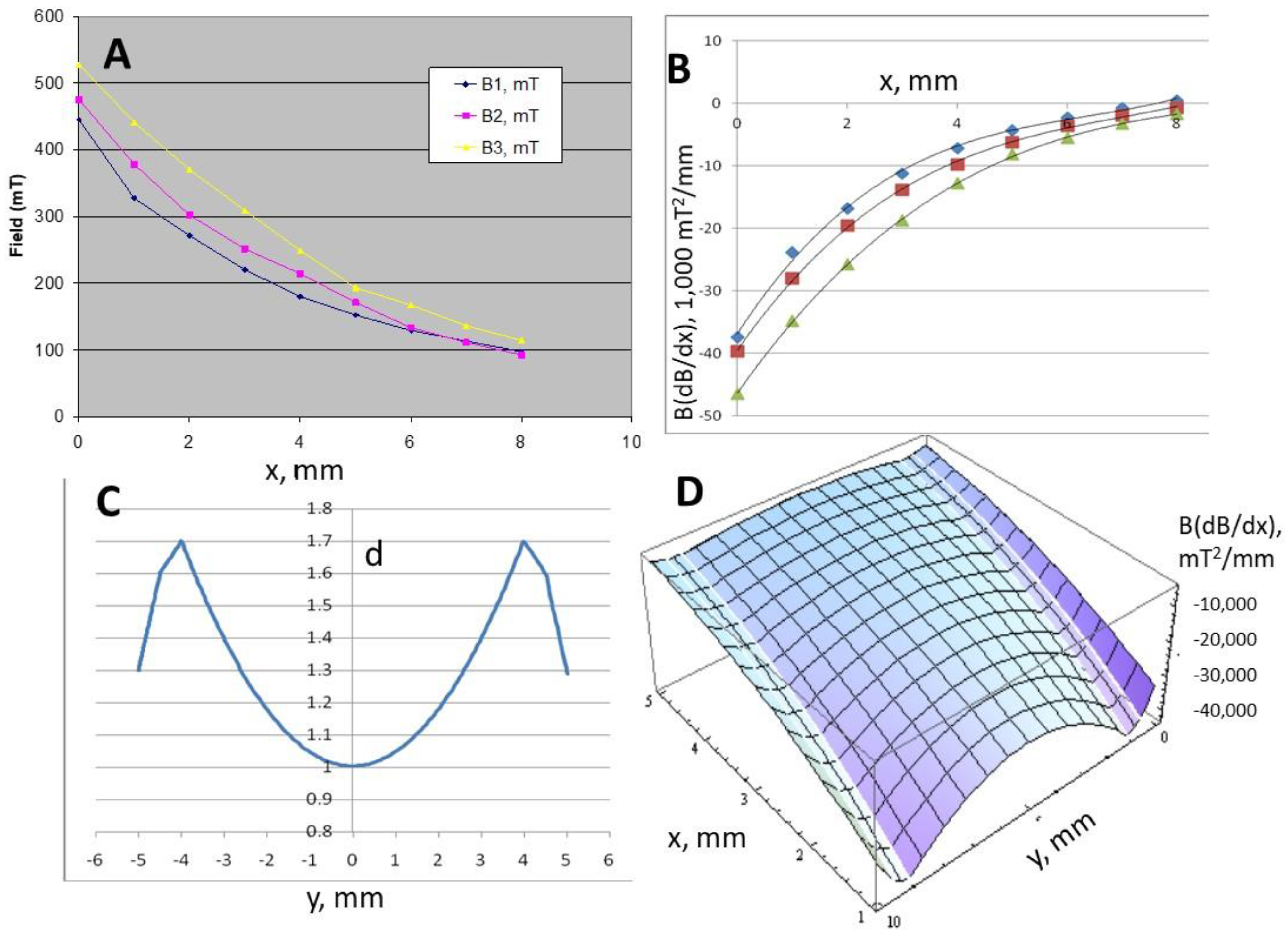
4.2.1. Magnetic Field Analysis

The spatial coordinates of a single stage in the magnetic trap are x = distance from the magnetic pole face (perpendicular to flow), y = direction of flow, z = down. For B∙▽B, experimental data shown in Figure 5A provide the relationship between B and distance x in this system. A simplified empirical relationship between B and x was obtained by curve fitting a 2nd degree polynomial in each case (numbering magnets from left to right in Figure 2). For the three magnet profiles, we obtain:

Magnet 1 B = 5.5541x² − 84.2x + 425.79
Magnet 2 B = 4.7240x² − 83.642x + 463.82
Magnet 3 B = 4.5509x² − 87.957x + 527.23

(8)

where B is in mT and x is in mm. To simplify the calculation, we consider magnetic force only in the x-direction, so B∙▽B can be simplified to B∙(dB/dx) for application to Equation (7) and the attractive (negative) magnetic pressure gradient plots of Figure 5B, which were obtained by multiplying each of these Equation (8) by its first derivative to obtain B(dB/dx) for the three magnets. Additionally, the magnetic field magnitude is not uniform along the y direction, so the above equations apply only at the center of the poleface. At other locations, they must be multiplied by a correction factor given by the theoretical distribution across the flat magnet pole face, as shown in Figure 5C. For these calculations, we consider the effective magnetic diameter to be 10 mm and use a channel length in the y-dimension of 10 mm, where magnetic force is present. An empirical factor function d is derived from this function, and used to calculate B(dB/dx) as function of y given in Equation (9):

d = 1.3 + 0.6y for (0 ≤ y ≤ 0.5) (for y in mm)
d = 1.6 + 0.2(y − 0.5) for (0.5 ≤ y ≤ 1)
d = 0.0437y² − 0.4368y + 2.0952 for (1 ≤ y ≤ 9)
d = 1.7 − 0.2(y − 9) for (9 ≤ y ≤ 9.5)
d = 1.6 − 0.6(y − 9.5) for (9.5 ≤ y ≤ 10)

(9)

Then, we have a modified version of Equation (7) for the x-velocity toward each magnet:

v_x = μ_md(B∙▽B)/μ_o

(10)

So for magnet 1, for example, we have:

v_x = 1.186 ∗ 10⁻⁵d(5.5541x² − 84.2x + 425.79)(11.1x − 84.2)

(11)

Applying these correction factors to a two-dimensional map of the magnetic pressure gradient gives the contours shown in Figure 5D, where x is the distance from the magnet pole face. This two-dimensional profile was used in calculations of trajectories of particles located anywhere within a 10 mm length of channel adjacent to magnet 1.

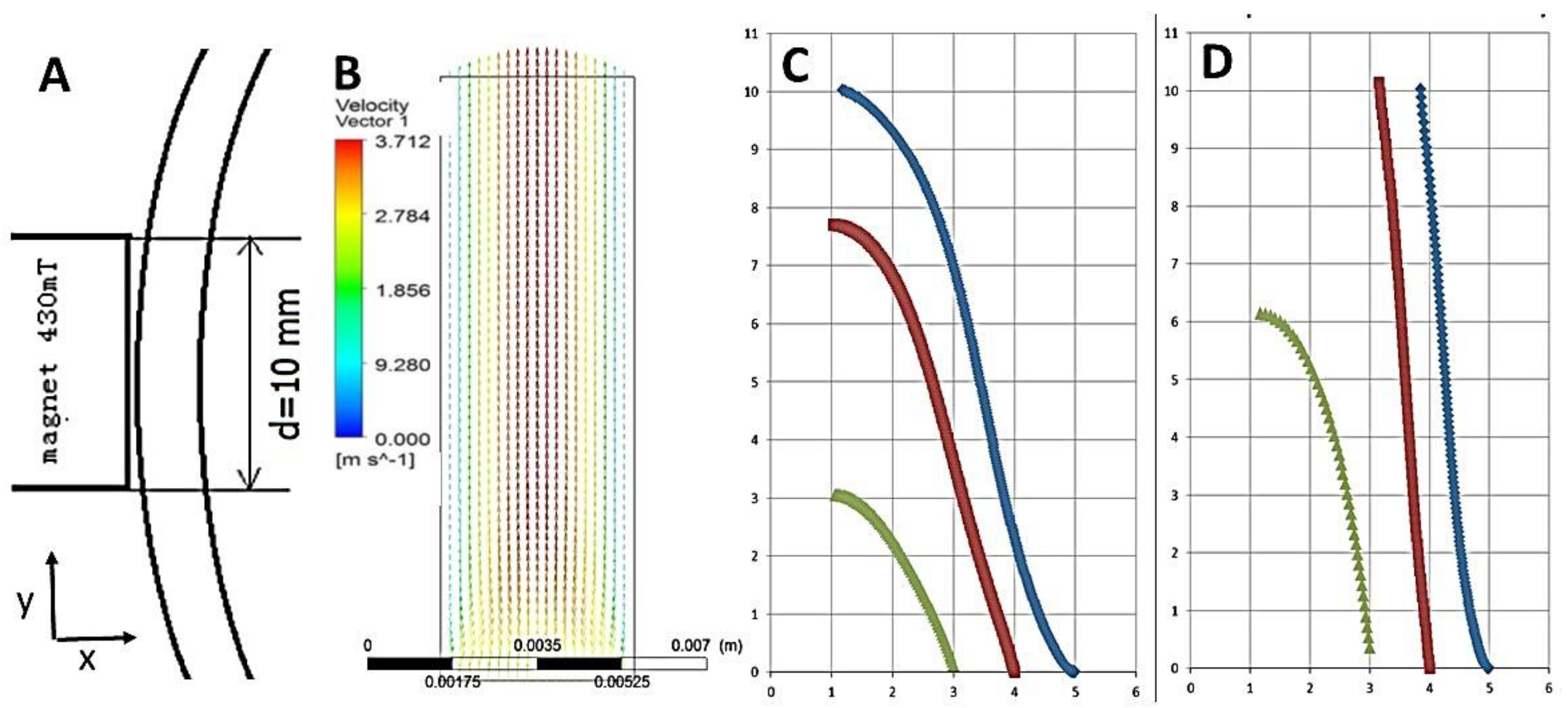
4.2.2. Computation of Magnetic Particle Trajectories

For velocity v_y, with the flow rate of 1 mL/min, we have: for divided channel, v = 0.5 mL/min, so in a channel with 5 mm height and 4 mm width, the average velocity = 0.04 cm/s = 0.4 mm/s. To obtain v_y the parabolic velocity profile v_y = ax² + bx + c is derived from the CFD simulation with boundary conditions: At the near and far walls of the channel, x = 1 and 5 mm, v_y = 0; and at x = 3 mm, v_y = v_max; and in general

v_y = v_max − a(x − 3)²

(12)

where 3 mm represents the position of the center of the channel.

As the channel can be considered as between two infinite planes, v(average) = (2/3)v_max and v_max = 0.6 mm/s. Thus, for a total input flow rate of 1 mL/min, the formula for v_y is

v_y = 0.6 − (x − 3)²0.15 mm/s

(13)

 and for a flow rate of 3 mL/min,

v_y = 1.8 − (x − 3)²0.45 mm/s

(14)

By representing the channel at a magnet interface as a 4 × 5 × 10 mm volume (Figure 6A), this velocity profile was computed by finite element analysis (Figure 6B), and referring to Figure 3, combined with the two-dimensional distribution of the ponderomotive force for magnet 1 shown in Figure 5D. From these calculations we obtain the function for particle velocity in directions x and y. Using a time step of 0.1 s, we obtain the track of a magnetic particle in the channel starting from three values of x when entering the magnetic field of magnet 1. These are shown in Figure 6C for a total flow rate of 1.0 mL/min and in 6D for a total flow rate of 3.0 mL/min. It is seen that all particles with the given magnetophoretic mobility (7.47 × 10⁻¹² m³/TAs) are captured at 1.0 mL/min, the flow rate of the static mixer, but not at 3.0 mL/min. Thus, the flow characteristics of the mixer and the trap are compatible, and cells to be trapped must have mobility equal to or greater than 7.5 × 10⁻¹² m³/TAs.

4.3. Experimental Test of In-Line Magnetic Capture

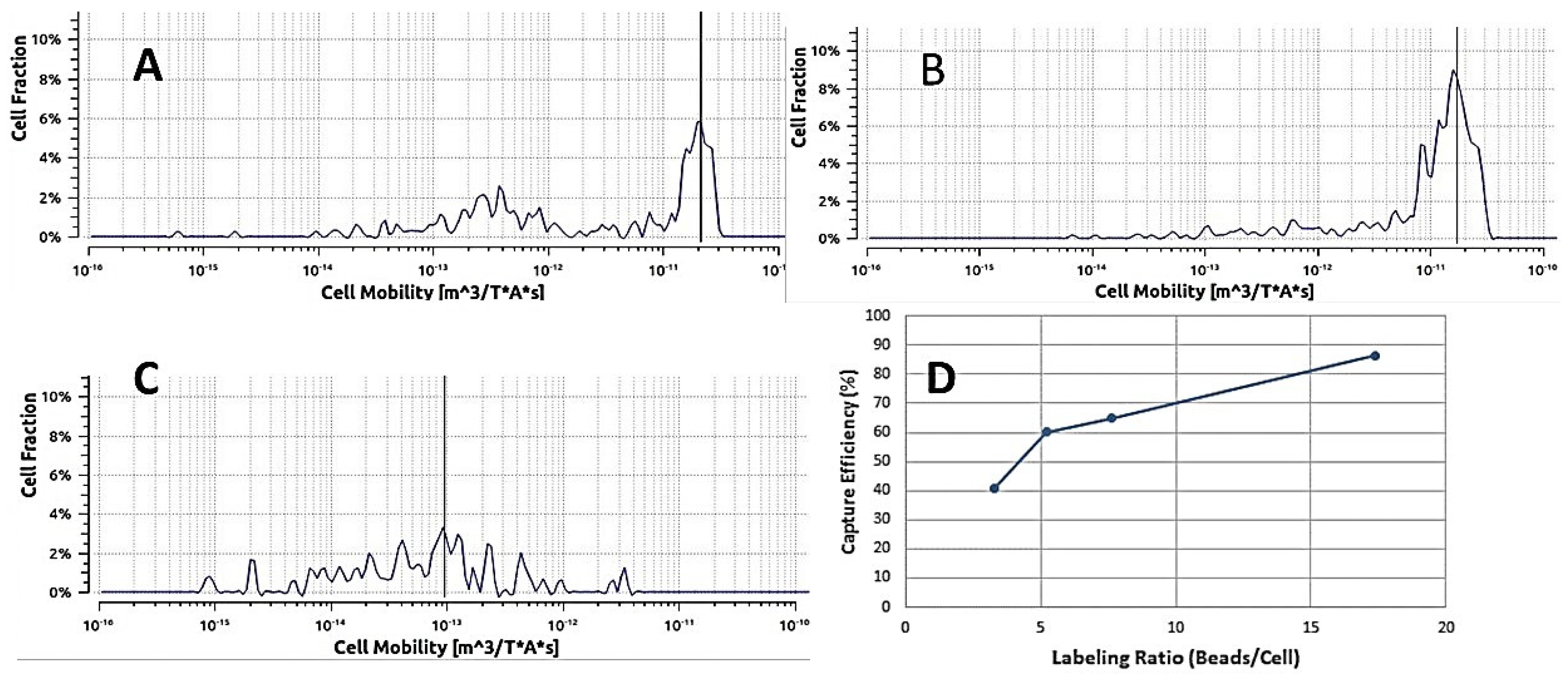
4.3.1. Magnetic Bead Capture Test

Proof-of-concept experiments were performed with a sample of Seradyne 3.27 μm diameter polystyrene beads with 14% iron oxide (the same beads as assumed in the simulations shown in Figure 6) were suspended in 10 mL of distilled water and pumped through the magnetic filter at 1 mL/min. The measured magnetophoretic mobility of these beads is 7.47 × 10⁻¹² m³/TAs, which is equal to the required mobility just demonstrated by computation. All beads were seen to be trapped by the first (weakest) magnet in the staged multimagnet series. Particle concentration was determined by hemacytometer counts. The concentration of particles entering the filter was 4.6 × 10⁸/mL, and the outflow contained <10⁴/mL (near the hemacytometer detection limit). Thus, a log-10-depletion of 4.7, or 99.998% capture of test beads was demonstrated.

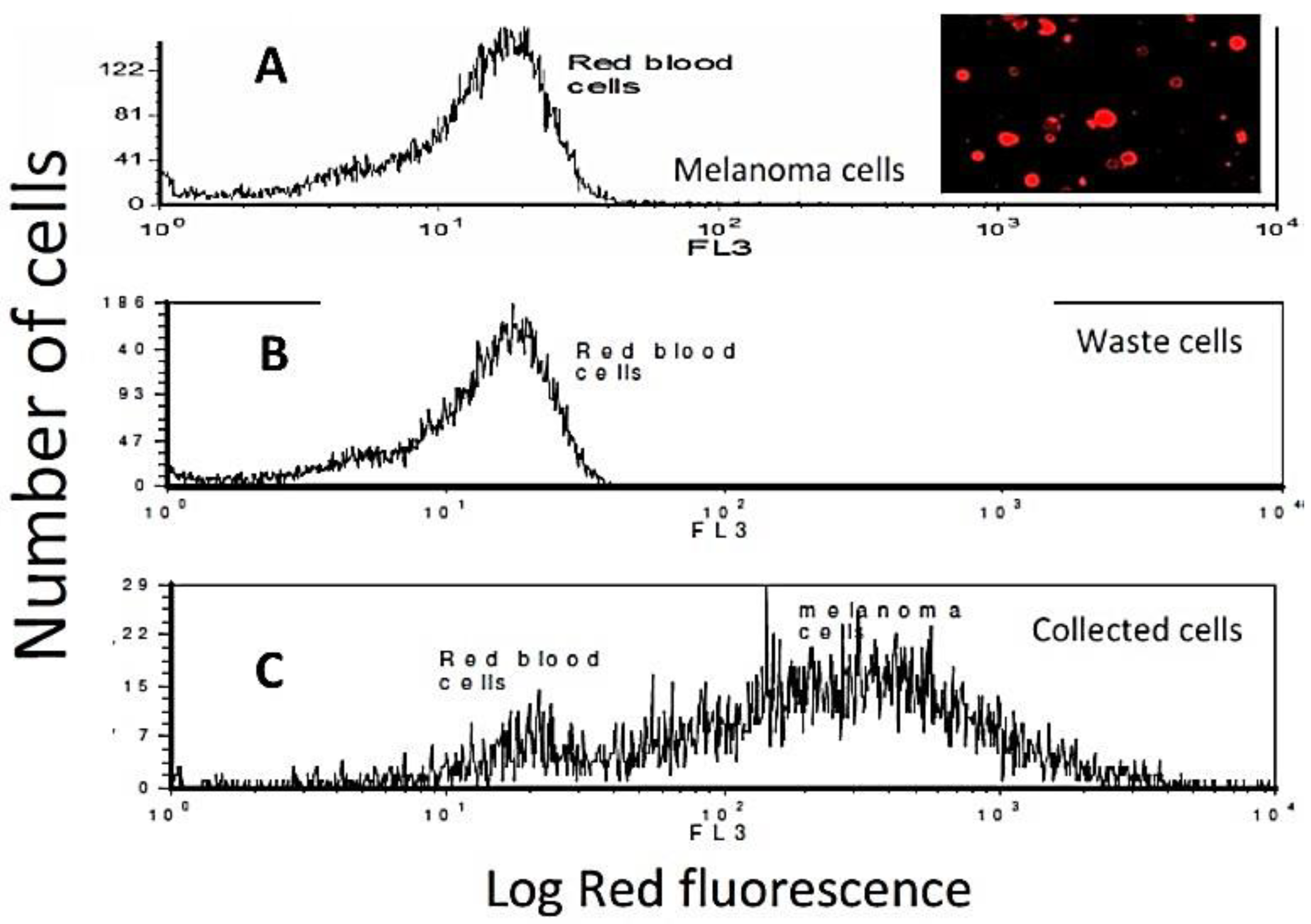
4.3.2. Labeled Cell Capture Test

Human melanoma cells (total of 10⁵) immunomagnetically labeled with 1.5 μm BioMag beads were suspended in 10 mL of PBS (see Materials and Methods–Cells), and were pumped through the magnetic trap with a flow rate of 0.8 mL/minute. The labeling ratio of magnetic particles to cells was 10:1. After pumping the cell suspension through the magnetic trap, all the magnetic particles and the labeled cells were trapped in the designated areas, while unlabeled cells escaped the trap and were collected at the outlet (waste). Magnetic trapping was highly efficient; 90 ± 7% of cells were counted in the trap and 10 ± 3% (labeled and non-magnetic) were collected in waste, and the process took less than 10 min.

4.3.3. Optimization

Chicken lymphoma cells at various concentrations, 1.3 × 10⁵ to 2.06 × 10⁶, were pre-labeled with Dynabeads at various labeling ratios (beads/cell), 5.2 to 17.4, as described above, and pumped through the trap at 1.0 mL/min. Waste (untrapped) cells were collected at the outlet and trapped cells were flushed with PBS from the trap after the removal of the magnetic fields. Figure 7 shows the magnetophoretic mobility histograms of the starting population of labeled cells (7A), as well as the captured (7B) and the waste (7C) samples. In this case, based on cell counts by hemacytometer, 62% of the input cells were captured in the trap. Given the above demonstrations and the data of Figure 7, it appears that some target cells were not sufficiently labeled to be captured. This finding affirms the importance of adequate labeling. The plot shown in Figure 7D demonstrates the effect of the labeling ratio on capture efficiency.

4.3.4. Experimental Test of In-Line Labeling Followed by Magnetic Capture

A comparison test was made between cells captured from the static in-line mixer and cells pre-labeled by the traditional shaker table method and the test results indicated that the static mixer is at least as proficient at the task of cell labeling for successful capture. In Figure 8, it is seen that both methods successfully labeled cells for trapping.

The two-parameter diagram (size vs. mobility) shown in Figure 8F indicates that cells trapped after in-line mixing have a similar size distribution as pre-labeled cells directly injected, although a higher number of total particles was analyzed relative to Figure 8D. By comparing the histograms of 8C and 8E, it appears that more cells were fully labeled by the in-line mixer. Furthermore, the magnetophoretic mobility of in-line labeled cells, 17 × 10⁻¹² m³/TAs, like that of pre-mixed cells, exceeds the required 7.5 × 10⁻¹² m³/TAs determined in the simulations (Figure 6) for successful trapping at 1.0 mL/min flow rate.

4.3.5. Capture of Target Cells from Whole Blood

The mixer and magnetic trap were tested using magnetic beads and citrated whole blood. The concentration of beads added to blood via the mixer did not vary from the first to the last 1-mL fraction collected from the mixer output during mixing tests.

For capture studies, cells were labeled with magnetic beads and quantum dots. The image in Figure 9A demonstrates the high affinity of the fluorescent QdotCD146 label for the CRL11147 target cells. The magnetic beads are expected to compete with the anti-CD146 Qdots for antibody sites on the outer membranes of the melanoma cells. The magnetic trap removed magnetically labeled CRL11146 cells and beads from whole blood, and released them into the rinse solution when the magnetic field was removed. Flushing nonmagnetically labeled cells (RBC & WBC) at 5 mL/min required less than 3 min. Flushing the captured cells out of the magnetic filter was shown to require less than 10 mL of fluid at a flow rate of 5 mL/min, and therefore required less than 2 min.

Initial experiments consisted of spiking whole blood with large numbers of the double-labeled melanoma cells using protocols described above (see Materials and Methods). The addition of 500,000 cells to 5 mL of whole blood leads to a spiking ratio of 1:10,000. The efficiency of labeling and trapping melanoma cells and depleting RBCs was investigated by loading the trap with 6 mL of spiked blood and washing the trap with 7 mL of PBS to collect waste. The magnetic field was removed, and melanoma cells were harvested in 7 mL of PBS. Analysis of fluorescence using a Coulter “Quanta” cytometer yielded the results shown in Figure 9.

In this figure, it is seen that there are very few “tick marks” ascending from the abscissa above FL3 = 50 in Figure 9A; these are the tiny number of melanoma cells spiked into 10,000 times as many RBCs. There were no fluorescent cells counted in the waste stream (9B), but the trapped cells were almost entirely fluorescent melanoma cells (9C). The RBCs are not fluorescent and do not contribute to the fluorescent cell count, but the RBCs were also in the minority in the trapped population, which is a goal.

Spiking melanoma cells into whole blood with a melanoma:RBC ratio of 1:1,000,000 was also studied. In a similar study to that just described, the Coulter “Quanta” flow cytometer counted zero fluorescent cells in the waste effluent from the magnetic trap, and in the counting volume used, counted 18–36 (range) fluorescent melanoma cells. These are the main results from a series of experiments that addressed this important question in a stepwise fashion: (1) Magnetic labeling and capture efficiency of pure melanoma cells labeled with 4.5 μm magnetic Dynabeads; (2) Magnetic labeling and capture efficiency of pure melanoma cells labeled with 1.5 μm magnetic Dynabeads; (3) Magnetic labeling and capture efficiency of melanoma cells at a high (1:10,000) ratio to RBCs in whole blood labeled with 1.5 μm magnetic Dynabeads; and (4) Magnetic labeling and capture efficiency of melanoma cells at a low (1:1,000,000) ratio in whole blood labeled with 1.5 μm magnetic beads. Using the available data, a synopsis of the results of these four tests is given in

Table 3. Summary of results of determination of labeling and capture efficiency of pure melanoma cells and cells spiked into whole blood.

Condition	Spiking Ratio	% Labeled, Captured	% to Waste
Pure, 4.5 μm beads	1:0	60	40
Pure, 1.5 μm beads	1:0	90 ± 7	10 ± 3
In blood, 1.5 μm beads	1:10,000	35 (?)	0–1
In blood, 1.5 μm beads	1:1,000,000	25–100 (range)	0–10 (range)

.

Based on these data, it appears that the expected low frequency of target cells in clinical specimens can be trapped, recovered and counted. Over the course of a series of experiments, counts of low numbers of cells have been made as necessary. When 10⁵ tumor cells were in the input, we found 90+% of the input tumor cells collected in the trap, and 10% in the waste. When only 5000 tumor cells were in the input, we found greater than 35% and possibly up to 100% trapping efficiency, with no melanoma cells counted in the waste. In a projected input containing 100 target cells we extrapolate that the per cent yield would be expected to be greater than 35%. No effort was made to optimize this number, so it should be considered a minimum. To reduce these uncertainties, future researchers will need to use sensitive cell detection methods such as an in-line microscope [2] or in-line sensitive flow cytometer [16].

5. Summary and Conclusions

By simultaneously simulating diffusion, flow rate, interfacial surface generation and sedimentation, optimal fluid mixing conditions, and hence optimal cell labeling can be demonstrated to occur in-line prior to the magnetic capture processes. The rate of particle diffusion between blood and reagent solutions is highly dependent on particle size. Simulations show that the blood sample and the reagent will reach a state of mass and velocity balance between stages 11 and 12, forming a well-mixed stream. At stage 20 in a 20-stage mixer, calculations indicated that quantum dots would require about 2 microseconds, and magnetic particles around 200 microseconds to diffuse to their target cells. The sedimentation rate for labeled cells was calculated, and found to be around 3.3 × 10⁻⁴ mm/s, resulting in negligible loss during the 600 s passage through the mixer. Results showed that a 20-stage static mixer can provide adequate time for blood and reagents to be well-mixed with negligible sedimentation loss at a flow rate of 1.0 mL/minute, and this was confirmed by experiements.

By simultaneously simulating magnetic transport, flow rate and sedimentation, optimal fluid conditions can be achieved to facilitate the in-line capture of magnetic cells from cell mixtures using a three-stage magnetic trap. At the desired flow rate of 1.0 mL/minute, it was shown by computation and experiment that all objects with magnetophoretic mobility greater than 7.5 × 10⁻¹² m³/TAs would be captured with nearly 100% efficiency. Quantum-dot labeled tumor cells doubly labeled with appropriate immunomagnetic beads have been captured and released for analysis by fluorescence flow cytometry, indicating a path to point-of-care circulating rare cell detection by semi-skilled operators with a portable device, such as depicted in Figure 10.

The foreseen workflow for a semi-skilled operator would consist of: (1) collecting up to 25 mL of whole blood into the heparinized or citrated sample syringe; (2) attaching the syringe to its coupling; (3) ensuring that all three syringes (sample, reagent, PBS) contain their respective fluids; (4) closing the lid; (5) waiting 45 min for automated processes to complete; (6) collecting bar-coded print-out from the microfluidic cytometer analysis; and (7) optionally obtaining magnetically collected cells in a tube at the outlet of the microfluidic cytometer. The missing component of the system is a miniature microfluidic flow cytometer, about 15 cm in maximum dimension, most of the technology for which has been implemented and tested [4,5,11,16]. The final phases of development require the ideal combination of the brilliance of qdots, the brightness of superluminescent LEDs and the sensitivity of state-of-the-art avalanche photodiodes (semiconductor photomultipliers).

References

1. Labib, M.; Kelley, S.O. Circulating tumor cell profiling for precision oncology. Mol. Oncol. 2021, 15, 1622–1646. [Google Scholar] [CrossRef] [PubMed]
2. Cristofanilli, M.; Budd, G.T.; Ellis, M.J.; Stopeck, A.; Matera, J.; Miller, M.C.; Reuben, J.M.; Doyle, G.V.; Allard, W.J.; Terstappen, L.W.; et al. Circulating tumor cells, disease progression, and survival in metastatic breast cancer. N. Engl. J. Med. 2004, 351, 781–791. [Google Scholar] [CrossRef] [PubMed] [Green Version]
3. Lee, Y.; Guan, G.; Bhagat, A.A. ClearCell® FX, a label-free microfluidics technology for enrichment of viable circulating tumor cells. Cytom. A 2018, 93, 1251–1254. [Google Scholar] [CrossRef] [PubMed] [Green Version]
4. Grafton, M.M.G.; Maleki, T.; Zordan, M.D.; Reece, L.M.; Byrnes, R.; Jones, A.; Todd, P.; Leary, J.F. Microfluidic MEMS Hand-Held Flow Cytometer. Proc. SPIE 2011, 7929, 79290C. [Google Scholar]
5. Maleki, T.; Fricke, T.; Quesenberry, J.T.; Todd, P.W.; Leary, J.F. Point-of-care, portable microfluidic blood analyzer system. Proc. SPIE 2012, 8251, 82510C. [Google Scholar] [CrossRef]
6. Plouffe, B.D.; Lewis, L.H.; Murthy, S.K. Computational design optimization for microfluidic magnetophoresis. Biomicrofluidics 2011, 5, 013413. [Google Scholar] [CrossRef] [PubMed] [Green Version]
7. Mohanty, S.; Baier, T.; Schönfeld, F. Three-dimensional CFD modelling of a continuous immunomagnetophoretic cell capture in BioMEMs. Biochem. Eng. J. 2010, 51, 110–116. [Google Scholar] [CrossRef]
8. Habibi, M.R.; Ghasemi, M. Numerical study of magnetic nanoparticles concentration in biofluid (blood) under influence of high gradient magnetic field. J. Magn. Magn. Mater. 2011, 323, 32–38. [Google Scholar] [CrossRef]
9. Allard, W.J.; Matera, J.; Miller, M.C.; Repollet, M.; Connelly, M.C.; Rao, C.; Tibbe, A.G.J.; Uhr, J.W.; Terstappen, L.W.M.M. Tumor cells circulate in the peripheral blood of all major carcinomas but not in healthy subjects or patients with nonmalignant diseases. Clin. Cancer Res. 2004, 10, 6897–6904. [Google Scholar] [CrossRef] [PubMed] [Green Version]
10. Paul, E.L. Handbook of Industrial Mixing-Science and Practice; John Wiley & Sons: Hoboken, NJ, USA, 2004; p. 399. [Google Scholar]
11. Todd, P.W.; Fricke, T.; Moyers, S. Cell Processing Cartridge for Miniature Cytometer. U.S. Patent 9,753,026 B1, 5 September 2017. [Google Scholar]
12. Zhou, C.; Boland, E.D.; Todd, P.W.; Hanley, T.R. Magnetic particle characterization—Magnetophoretic mobility and particle size. Cytom. Part A 2016, 89, 585–593. [Google Scholar] [CrossRef] [PubMed] [Green Version]
13. Zhou, C.; Qian, Z.; Choi, Y.S.; David, A.E.; Todd, P.; Hanley, T.R. Application of magnetic carriers to two examples of quantitative cell analysis. J. Magn. Magn. Mater. 2017, 427, 25–28. [Google Scholar] [CrossRef] [Green Version]
14. Zborowski, M.; Chalmers, J.J. (Eds.) Magnetic Cell Separation; Elsevier: Amsterdam, The Netherlands, 2008. [Google Scholar]
15. Richardson, J.F.; Zaki, W.N. Sedimentation and fluidisation: Part I. Trans. Inst. Chem. Eng. 1954, 38, 33. [Google Scholar] [CrossRef]
16. Leary, J.F. Design of portable microfluidic cytometry devices for rapid medical diagnostics in the field. Imaging Manip. Anal. Biomol. Cells Tissues XVII 2019, 10881, 108810B. [Google Scholar] [CrossRef]
17. Liberti, P.A.; Rao, C.; Terstappen, L.W.M.M. Optimisation of ferrofluids and protocols for the enrichment of breast tumor cells in blood. J. Magn. Magn. Mater. 2001, 225, 301–307. [Google Scholar] [CrossRef]
Figure 1. Static mixing device and principle. (A): Image of a single-use commercial (Loctite) static mixer, 10 × 150 mm. (B): Depiction of interfacial surface generation (ISG) downstream of each baffle in sequence.
Magnetochemistry 08 00005 g001
Figure 2. Three-stage magnetic trap. (A). Photo of trap showing paired channels with collection curves and collection magnets. Magnets are 10 mm in diameter, and the total internal volume (both channels) is 3.8 mL. Captured cells are collected by flushing the channels after removing the single-use channel assembly from the magnets. Rectangle shows region of interest for magnetic calculations. (B). Mesh was applied to the channels of the trap for CFD using FLUENT.
Magnetochemistry 08 00005 g002
Figure 3. Flow chart for CFD simulation showing the blend of ICEM, FLUENT and user-defined analytical functions.
Magnetochemistry 08 00005 g003
Figure 4. Results of simulations combining blood and reagent solution. (A): View from the entrance of the mixer showing volume fraction of the phases (blood phase in red, reagent phase in blue). (B): End-to-end view of blood phase volume fraction as a function of mixing stage showing center cut at stage 10 where mixing is not complete. The 83% blood volume complete mix is shown as orange (see color scale). (C): View from downstream end showing blood volume fraction in cross sections at the outlet and stage 18 where mixing is complete. Homogeneous orange distribution is consistent with 83%/17% V/V complete blend of blood with reagent. Beyond stage 16, the reagent phase is a constant 17%. (D): Velocity stream lines within the static mixer stages near the inlet. Lower volumetric flow rate of the reagent phase is seen as dark blue streamlines at the inlet (see color scale), but it does not stagnate. Beyond stage 16, streamline velocities are very similar, at about 2.6 cm/s.
Magnetochemistry 08 00005 g004
Figure 5. Magnetic field analysis. (A): Measured magnetic flux density B outward from the center of the pole pieces of magnets 1, 2 and 3. (B): Ponderomotive force versus distance from the poleface of each of the three magnets; negative value indicates the force’s direction (negative x velocity). The ordinate is in units of 1000 mT2/mm, negative because it is attractive. (C): Multiplier d for Equation (9) as a function of radial distance from the center of the magnetic pole face. (D): Magnetic ponderomotive force field as given by Equation (10), where d is a function of y. Units are mm and mT2/mm.
Magnetochemistry 08 00005 g005
Figure 6. Computation of labeled cell trajectories. (A): Region of interest selected for trajectory analysis as shown in Figure 2A (rectangle). (B): Velocity vector in the region of interest for magnet particle analysis (2-D model). Streamline of magnetic trap with inlet stream velocity of 5.32 mm/s. (C): Calculated particle tracks of 3.27 μm diameter polystyrene magnetic beads having magnetophoretic mobility µm = 7.47 × 10⁻¹² m3/TAs, (see “Reagents and Solutions” above) at a flow rate of 1.0 mL/min. The magnet face is at x = 0 mm and channel walls are at x = 1 mm and x = 5 mm, channel length is 10 mm. Particles start from x = 3, 4 and 5 mm, respectively. All particles are captured. (D): Same particle tracks, with the flow rate increased to 3 mL/min. The particles most distant from the magnet are not captured at the first stage but have been moved to a streamline closer to subsequent magnets for potential downstream capture.
Magnetochemistry 08 00005 g006
Figure 7. Results of tumor cell capturing experiments. (A): Magnetophoretic mobility histogram of starting population of chicken lymphoma cells pre-labeled with Dynabeads showing broad distribution of unlabeled cells and high-mobility peak at 20 × 10−12 m3/TAs of fully labeled cells. (B): Mobility histogram of trapped cells showing nearly complete depletion of unlabeled cells. (C): Mobility histogram of untrapped cells collected at the outlet consisting of only unlabeled cells and showing complete depletion of labeled cells. (D): Effect of labeling ratio on the efficiency of capture. All labeled cells are captured, and unlabeled cells are not.
Magnetochemistry 08 00005 g007
Figure 8. Magnetic analysis of cells collected in the trap after labeling by standard shake table method and by in-line mixing affirming the results of Figure 4 (complete mixing). (A): Magnetophoretic mobility histogram of unlabeled CRL-211, DT40 chicken lymphoma cells showing a typical broad distribution for unlabeled cells. (B): Two-parameter plot of diameter (in pixels) vs. mobility (linear scale) showing very few objects with non-zero mobility. (C): Mobility histogram of cells labeled for 20 min with immunomagnetic Dynabeads on a rocker table. (D): Two-parameter plot for labeled cells showing the categories counted: 1 = unlabeled cells (depleted vs. control due to labeling); 2 = debris; 3 = unbound Dynabeads; 4 = magnetically labeled cells. (E): Mobility histogram of cells labeled in 10 min with reagent solution and cell suspension flowing through the in-line mixer at 1.0 mL/min. (F): Two-parameter plot for labeled cells harvested from the in-line mixer showing abundance of labeled cells with a cluster at mobility = 17 × 10−12 m3/Tas, as also seen on the histogram (8E).
Magnetochemistry 08 00005 g008
Figure 9. Flow cytometric analysis of magnetic Qdot-labeled human melanoma cells spiked into human whole blood at a ratio of 1:10,000. (A): Fluorescence histograms of the cell mixture before magnetic separation and color fluorescence micrograph demonstrate an example of the red fluorescent anti-CD146 Qdot labeled CRL11147 cell populations. (B): The RBCs collected in the waste. No melanoma cells could be counted. (C): Cells collected from the trap after removal of the magnetic field. Cells below FL3 = 50 are not fluorescent, and are mainly RBCs.
Magnetochemistry 08 00005 g009
Figure 10. (Left): Concept for an automated point-of-care portable rare cell detection system using the components developed in this research. (Right): Concept for an add-on miniature dedicated flow cytometer [16] with a single-use microfluidics cartridge [4,11] to receive captured cells flushed out of the magnetic trap.
Magnetochemistry 08 00005 g010