
Analysis of the Mutual Impedance of Coils Immersed in Water


Abstract
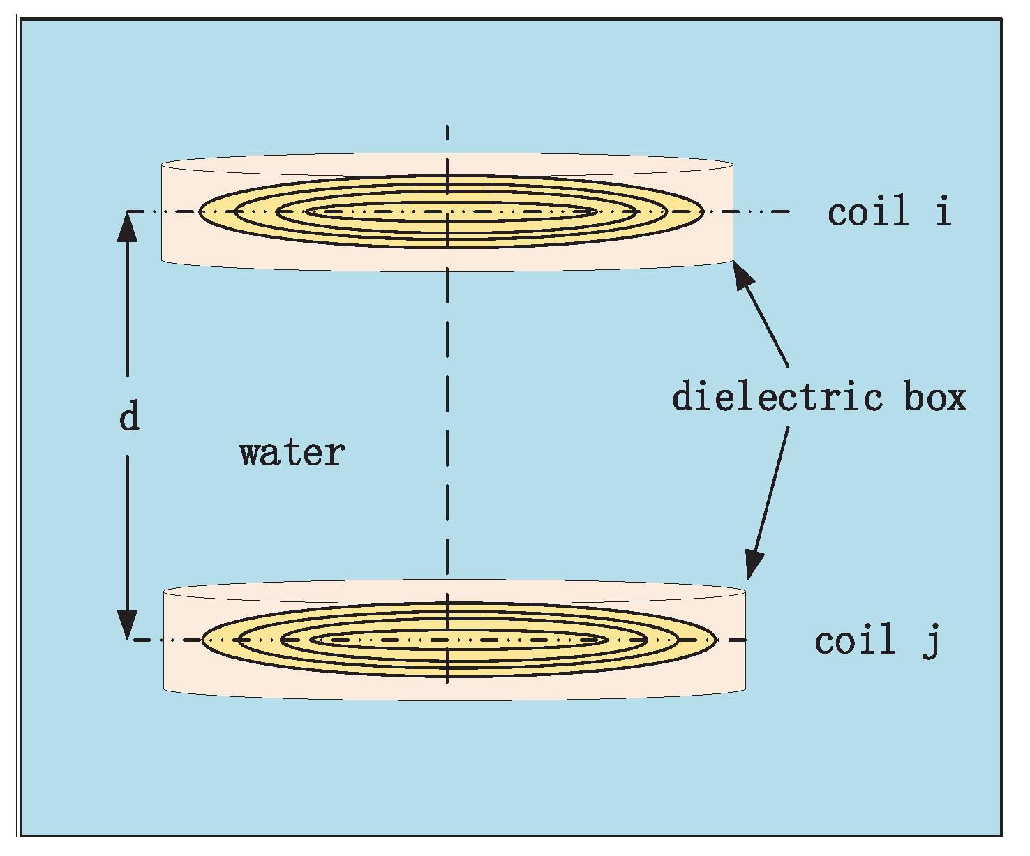
:1. Introduction
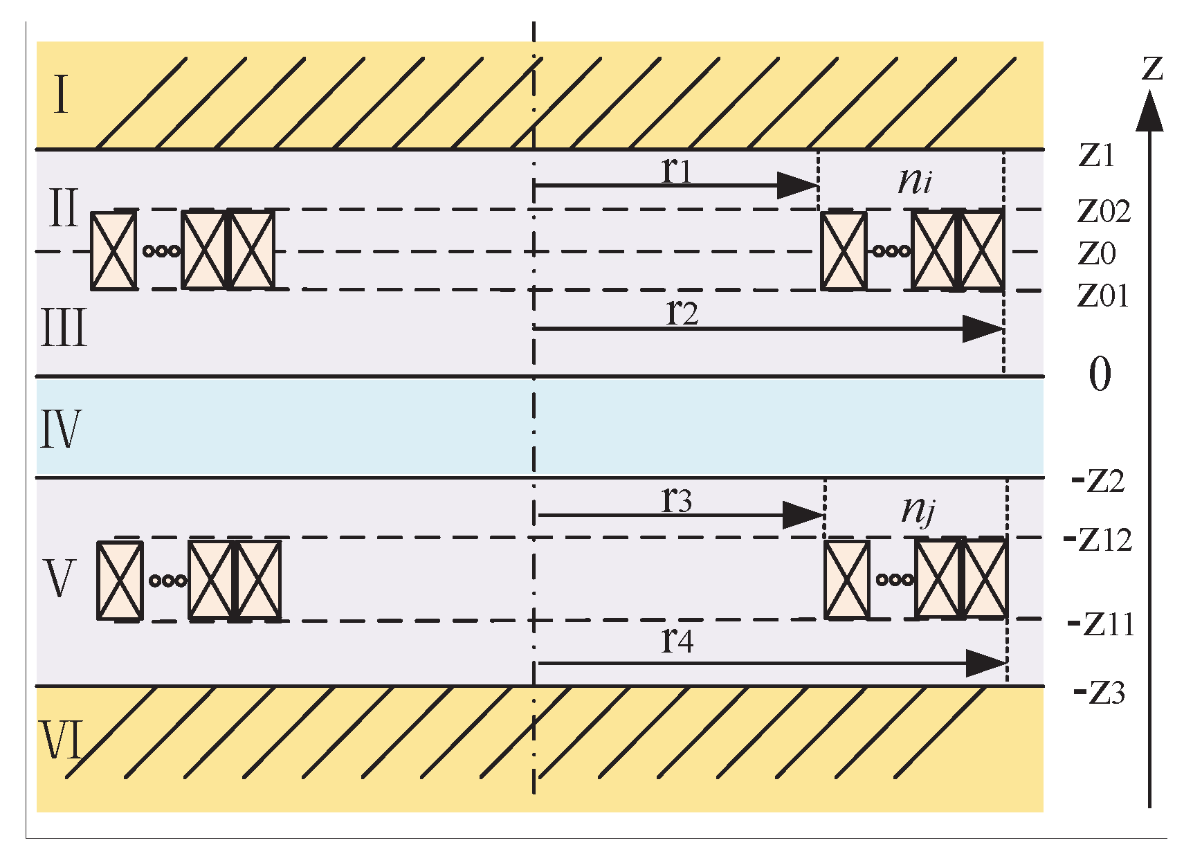
2. Mutual Impedance of Two Coils of Filamentary Currents
3. Convergence Analysis of the Model
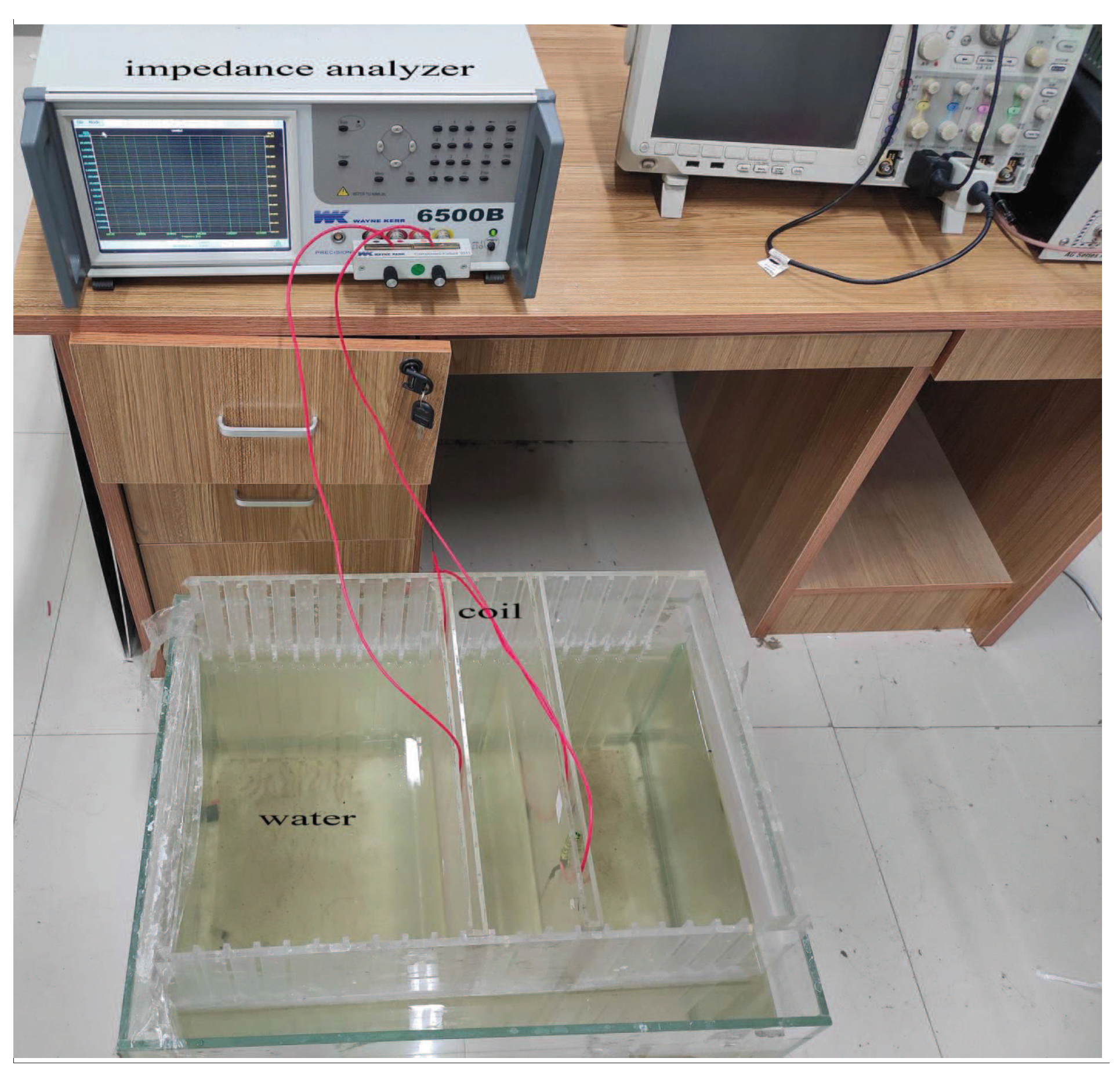
4. Experimental Results and Discussion
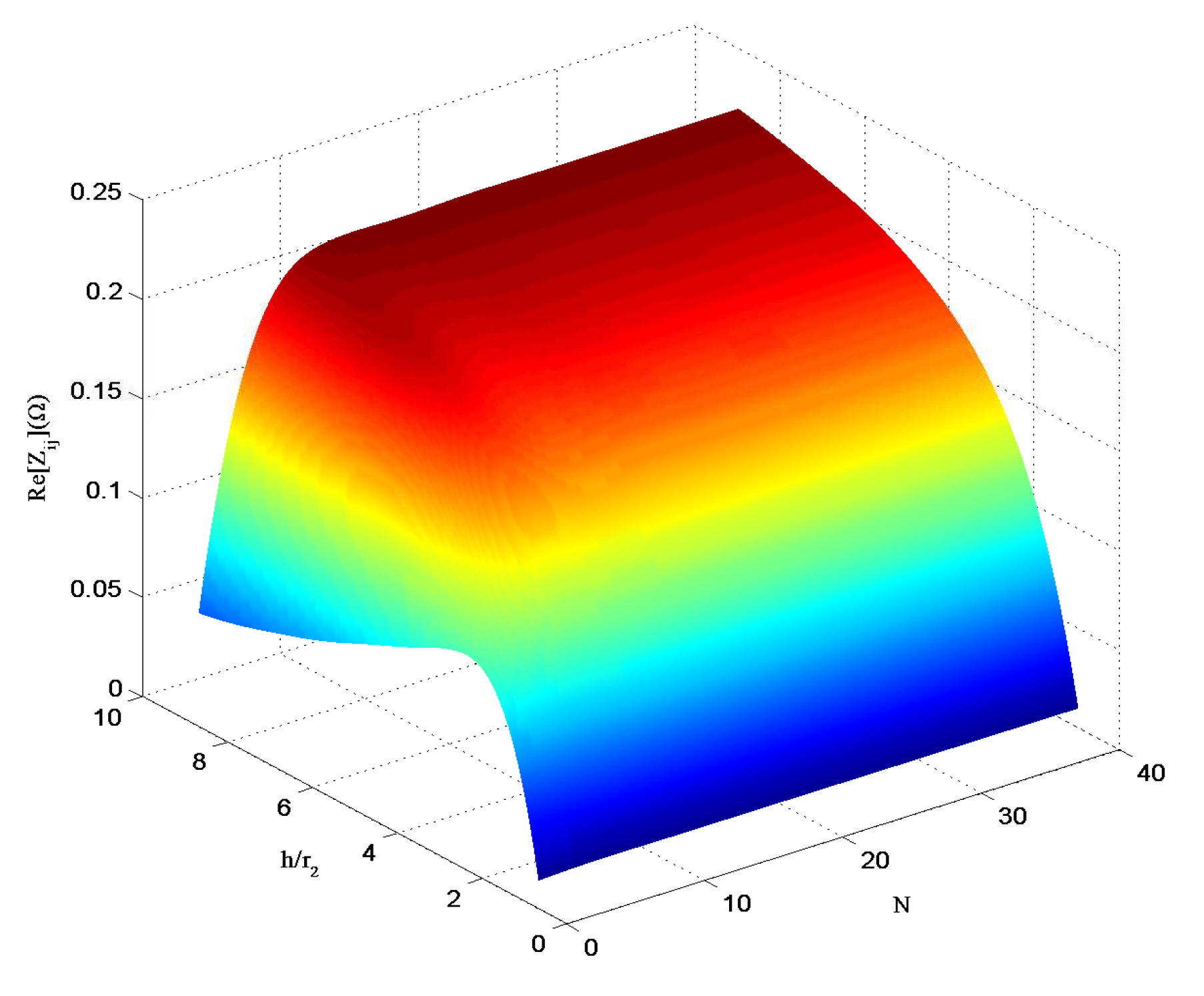
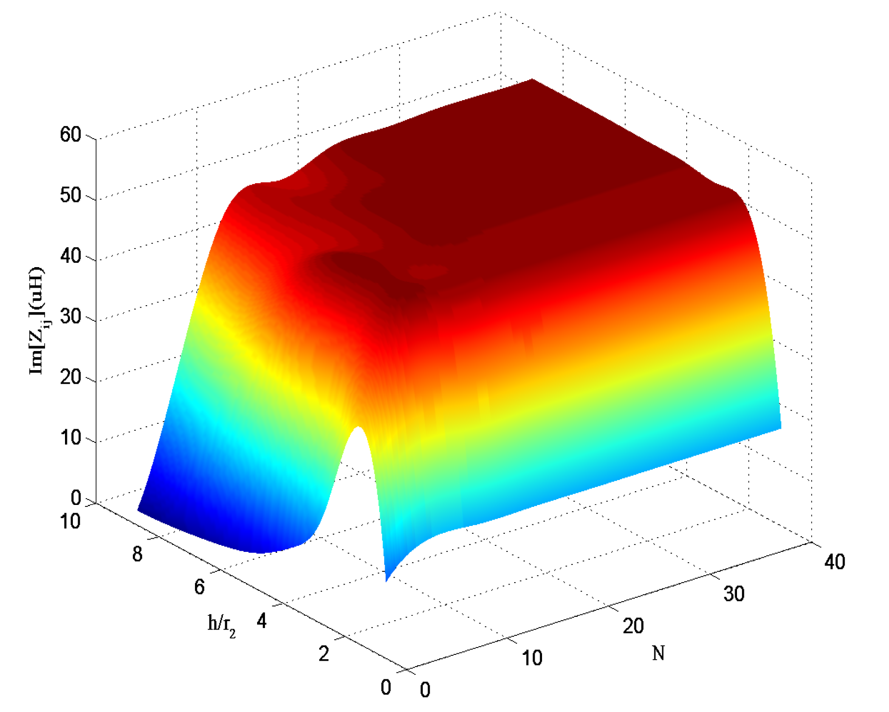
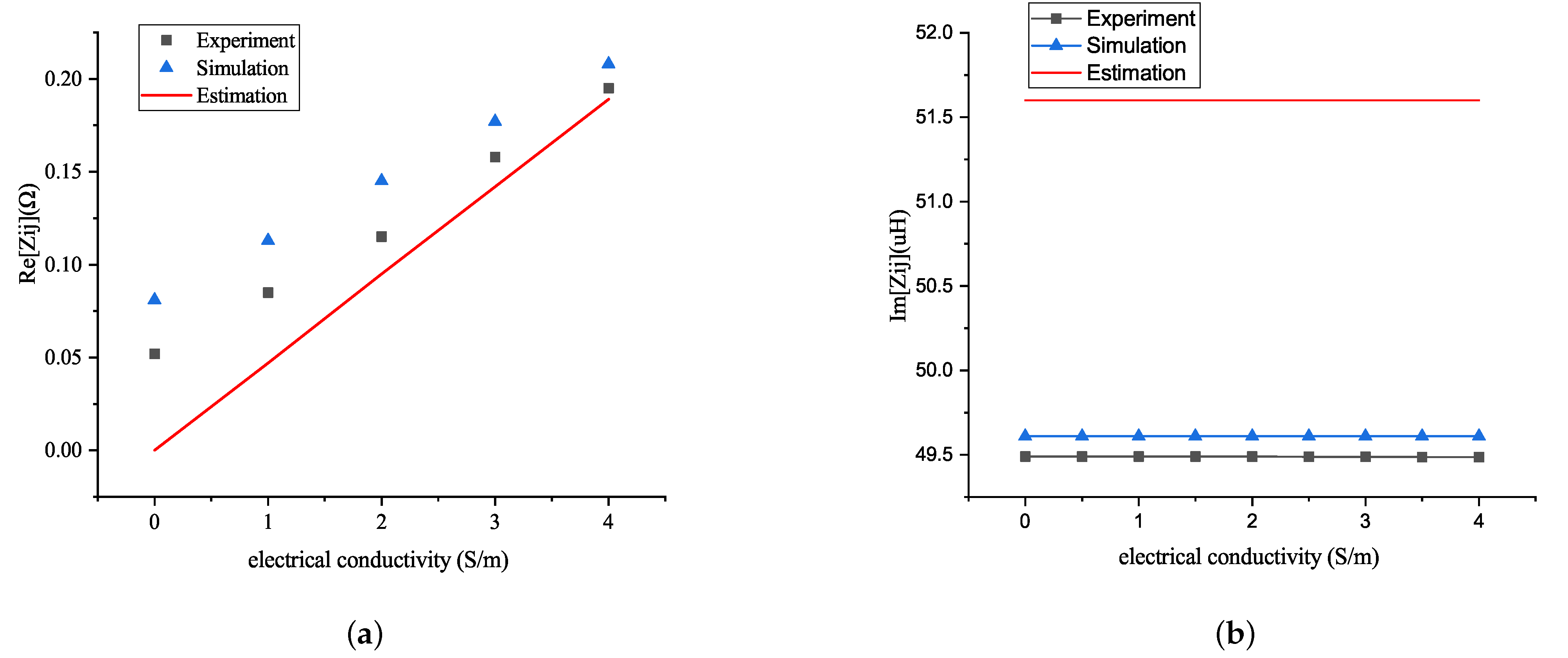
4.1. Influence of the Conductivity in the Mutual Impedance
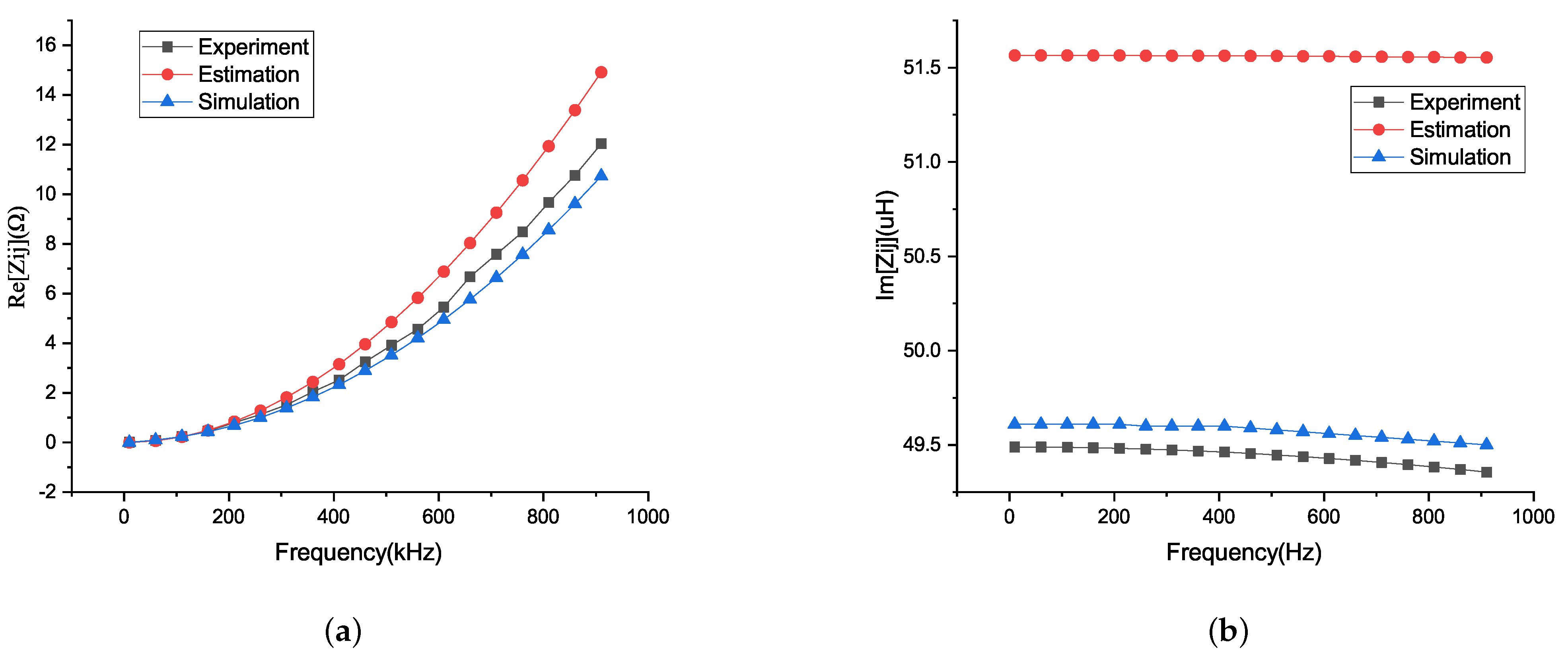
4.2. Influence of Frequency in the Mutual Impedance
4.3. Variation of Mutual Impedance with Axial Displacement
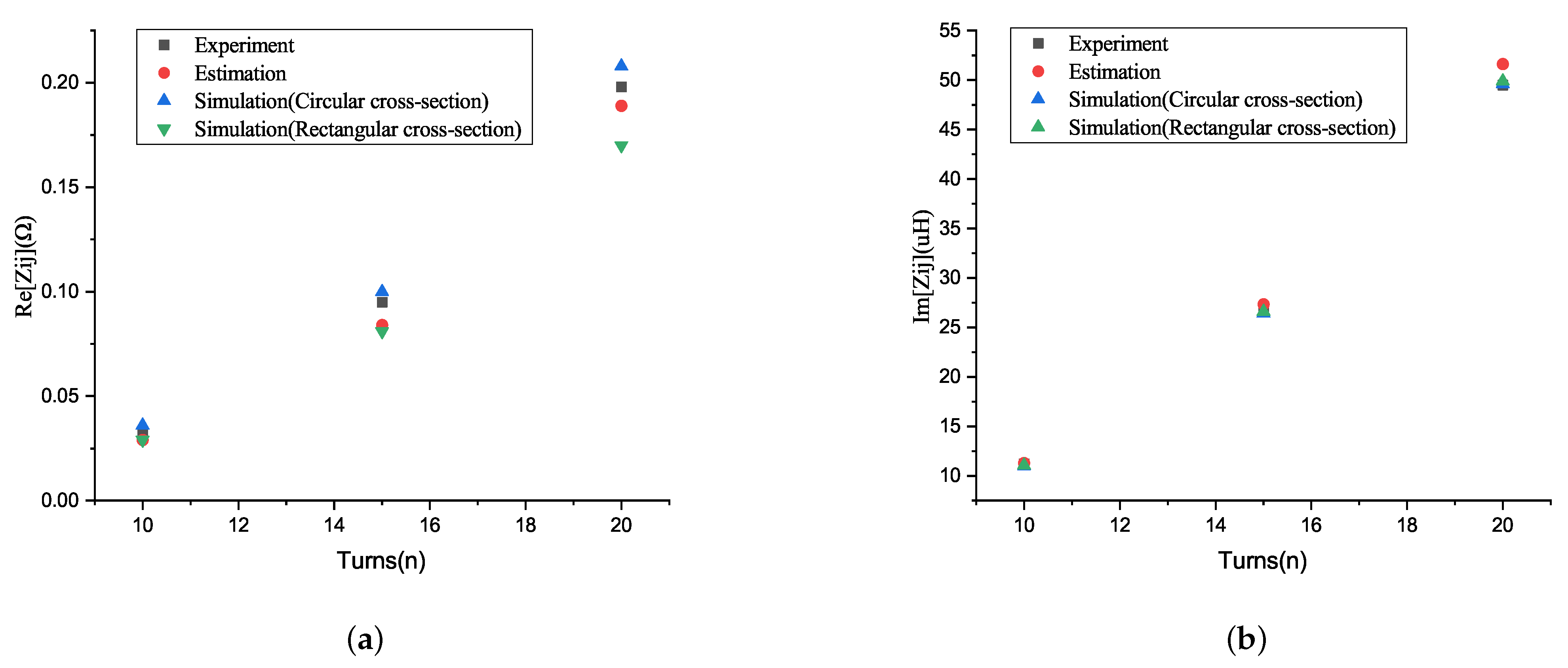
4.4. Error Analysis Introduced by the Assumption of Cross-Section
4.5. Discussion
5. Conclusions
Author Contributions
Funding
Institutional Review Board Statement
Informed Consent Statement
Data Availability Statement
Conflicts of Interest
References
- Miorelli, R.; Reboud, C.; Theodoulidis, T.P.; Poulakis, N.; Lesselier, D. Efficient modeling of ECT signals for realistic cracks in layered half-space. IEEE Trans. Magn. 2013, 49, 2886–2992. [Google Scholar] [CrossRef]
- Tan, X.; Sun, Z.; Akyildiz, I.F. Wireless Underground Sensor Networks: MI-based communication systems for underground applications. IEEE Antennas Propag. Mag. 2015, 57, 74–87. [Google Scholar] [CrossRef]
- Zhang, Z.; Pang, H.; Georgiadis, A.; Cecati, C. Wireless Power Transfer-An Overview. IEEE Trans. Ind. Electron. 2019, 66, 1044–1058. [Google Scholar] [CrossRef]
- Kiani, M.; Jow, U.M.; Ghovanloo, M. Design and Optimization of a 3-Coil Inductive Link for Efficient Wireless Power Transmission. IEEE Trans. Biomed. Circuits Syst. 2011, 5, 579–591. [Google Scholar] [CrossRef] [PubMed] [Green Version]
- Zhang, X.; Yuan, Z.; Yang, Q.; Li, Y.; Zhu, J.; Li, Y. Coil Design and Efficiency Analysis for Dynamic Wireless Charging System for Electric Vehicles. IEEE Trans. Magn. 2016, 52, 1. [Google Scholar] [CrossRef]
- Yan, Z.; Zhang, Y.; Kan, T.; Lu, F.; Zhang, K.; Song, B.; Mi, C.C. Frequency Optimization of a Loosely Coupled Underwater Wireless Power Transfer System Considering Eddy Current Loss. IEEE Trans. Power Electron. 2019, 66, 3468–3476. [Google Scholar] [CrossRef]
- Kan, T.; Mai, R.; Mercier, P.P.; Mi, C.C. Design and Analysis of a Three-Phase Wireless Charging System for Lightweight Autonomous Underwater Vehicles. IEEE Trans. Power Electron. 2018, 33, 6622–6632. [Google Scholar] [CrossRef]
- McGinnis, T.; Henze, C.P.; Conroy, K. Inductive power system for autonomous underwater vehicles. OCEANS 2007, 2007, 1–5. [Google Scholar]
- Zhou, J.; Li, D.J.; Chen, Y. Frequency selection of an inductive contactless power transmission system for ocean observing. Ocean Eng. 2018, 60, 175–185. [Google Scholar] [CrossRef]
- Zhong, W.; Hui, S.Y.R. Maximum Energy Efficiency Operation of Series-Series Resonant Wireless Power Transfer Systems Using On-Off Keying Modulation. IEEE Trans. Power Electron. 2018, 33, 3595–3603. [Google Scholar] [CrossRef]
- Kim, J.; Kim, J.; Kong, S.; Kim, H.; Suh, I.S.; Suh, N.P.; Cho, D.H.; Kim, J.; Ahn, S. Coil Design and Shielding Methods for a Magnetic Resonant Wireless Power Transfer System. Proc. IEEE 2013, 101, 1332–1342. [Google Scholar] [CrossRef]
- Babic, S.; Sirois, F.; Akyel, C.; Girardi, C. Mutual Inductance Calculation Between Circular Filaments Arbitrarily Positioned in Space: Alternative to Grover’s Formula. IEEE Trans. Magn. 2010, 46, 3591–3600. [Google Scholar] [CrossRef]
- Burke, S.K.; Ibrahim, M.E. Mutual impedance of air-cored coils above a conducting plate. J. Phys. D Appl. Phys. 2004, 37, 1857–1868. [Google Scholar] [CrossRef]
- Vallecchi, A.; Chu, S.; Solymar, L.; Stevens, C.J.; Shamonina, E. Coupling between coils in the presence of conducting medium. IET Microwaves Antennas Propag. 2019, 13, 55–62. [Google Scholar] [CrossRef]
- Acero, J.; Carretero, C.; Lope, I.; Alonso, R.; Burdio, J.M. Analysis of the Mutual Inductance of Planar-Lumped Inductive Power Transfer Systems. IEEE Trans. Ind. Electron. 2013, 60, 410–420. [Google Scholar] [CrossRef]
- Ma, J.; Zhang, X.; Huang, Q.; Cheng, L.; Lu, M. Experimental Study on the Impact of Soil Conductivity on Underground Magneto-Inductive Channe. IEEE Antennas Wirel. Propag. Lett. 2015, 14, 1782–1785. [Google Scholar] [CrossRef]
- Yan, Z.; Song, B.; Zhang, K.; Wen, H.; Mao, Z.; Hu, Y. Eddy current loss analysis of underwater wireless power transfer systems with misalignments. J. Appl. Phys. 2018, 8, 101421. [Google Scholar] [CrossRef] [Green Version]
- Schauber, M.J.; Newman, S.A.; Goodman, L.R.; Suzuki, I.S.; Suzuki, M. Measurement of mutual inductance from frequency dependence of impedance of AC coupled circuit using digital dual-phase lock-in amplifier. Am. J. Phys. 2008, 76, 129. [Google Scholar] [CrossRef] [Green Version]
- Jash, A.; Roy, N.; Bag, B.; Banerjee, S.S. A two-coil mutual inductance technique to study the conductivity of metal and measurement of the superconducting transient temperature. AIP Conf. Proc. 2018, 1942, 060026. [Google Scholar]
- Theodoulidis, T.P.; Kriezis, E.E. Series expansions in eddy current nondestructive evaluation. J. Mater. Process. Technol. 2005, 161, 343–347. [Google Scholar] [CrossRef]
- Theodoulidis, T.P.; Bowler, J.R. The truncated region eigenfunction expansion method for the solution of boundary value problems in eddy current nondestructive evaluation. Rev. Prog. Quant. Nondestruct. Eval. 2004, 24, 403–408. [Google Scholar]


Publisher’s Note: MDPI stays neutral with regard to jurisdictional claims in published maps and institutional affiliations. |
© 2021 by the authors. Licensee MDPI, Basel, Switzerland. This article is an open access article distributed under the terms and conditions of the Creative Commons Attribution (CC BY) license (https://creativecommons.org/licenses/by/4.0/).
Share and Cite
Liu, P.; Gao, T.; Mao, Z. Analysis of the Mutual Impedance of Coils Immersed in Water. Magnetochemistry 2021, 7, 113. https://doi.org/10.3390/magnetochemistry7080113
Liu P, Gao T, Mao Z. Analysis of the Mutual Impedance of Coils Immersed in Water. Magnetochemistry. 2021; 7(8):113. https://doi.org/10.3390/magnetochemistry7080113
Chicago/Turabian StyleLiu, Peizhou, Tiande Gao, and Zhaoyong Mao. 2021. "Analysis of the Mutual Impedance of Coils Immersed in Water" Magnetochemistry 7, no. 8: 113. https://doi.org/10.3390/magnetochemistry7080113
APA StyleLiu, P., Gao, T., & Mao, Z. (2021). Analysis of the Mutual Impedance of Coils Immersed in Water. Magnetochemistry, 7(8), 113. https://doi.org/10.3390/magnetochemistry7080113