Structure–Property Relationships for Weak Ferromagnetic Perovskites

Abstract

Despite several decades of active experimental and theoretical studies of rare-earth orthoferrites, the mechanism of the formation of their specific magnetic, magnetoelastic, optical, and magneto-optical properties remains a subject of discussion. This paper provides an overview of simple theoretical model approaches to quantitatively describing the structure–property relationships—in particular, the interplay between FeO₆ octahedral deformations/rotations and the main magnetic and optic characteristics, such as Néel temperature, overt and hidden canting of magnetic sublattices, magnetic and magnetoelastic anisotropy, and optic and photoelastic anisotropy.

1. Introduction

The rare-earth orthoferrites of the general formula RFeO₃ (R = Y, or rare-earth ion) have attracted and continue to attract the particular attention of researchers for several decades owing to their weak ferromagnetism, remarkable magneto-optical properties, spin-reorientation transitions between antiferromagnetic phases, high velocity of domain walls, and many other properties. Their physical properties remain a focus of considerable research due to their promising applications in innovative spintronic devices; furthermore, they contribute to an emerging class of materials, i.e., multiferroics with strong magnetoelectric (ME) coupling.

The rare-earth orthoferrites RFeO₃ (space group D${}_{2h}^{16}$) have a distorted perovskite structure with only one type of Fe${}^{3+}$ ion octahedrally coordinated with six O${}^{2-}$ ions [1,2]. Their complex non-collinear magnetic structures and magnetic phase transitions are primarily due to the combination of the antiferromagnetic (AFM) exchange interaction with the Dzyaloshinskii–Moriya (DM) antisymmetric exchange interaction.

Despite the impressive advances in modern ab-initio band structure computation techniques, as well as various quantum-chemistry cluster computation methods, for the majority of practically important systems, these methods give only a rather rough picture of the electronic structure and the energy spectrum that can, at best, serve only as a suggestion for developing an adequate theory. One of the most recent and illustrative examples of ab-initio calculations is given in Ref. [3], the authors of which performed first principles simulations for the structural, elastic, vibrational, electronic, and optical properties of orthorhombic samarium orthoferrite SmFeO${}_3$ within the framework of density functional theory. However, such calculations encounter great difficulties in describing the more “subtle” effects of magnetic, magnetoelastic, and optical anisotropy [4].

In this paper, we apply simple theoretical approaches to quantitatively evaluate the interplay between FeO${}_6$ octahedral deformations/rotations and the main magnetic and optic characteristics, such as Néel temperature, overt and hidden canting of magnetic sublattices, magnetic and magnetoelastic anisotropy, and optic and photoelastic anisotropy. These involve describing a distorted (low-symmetry) structure as arising from a (high-symmetry) parent structure with one or more static symmetry-breaking structural distortions.

Knowledge of the structure–property relationships is required both to elucidate the nature of their physical properties and to accelerate materials’ discoveries.

Accessibility to computational methods makes the distortion-mode analysis powerful, because it is possible to independently study various distortions and directly assess their role in forming the electronic structure and physical properties.

The structure–property relationships in ABO${}_3$ perovskites exhibiting octahedral rotations and distortions were studied using group theoretical methods [5]. The relationship between the rotation angles of octahedra and bond-strength energy in crystals with a perovskite structure was studied in Ref. [6]. However, there are practically no examples of using structure–property relationships to describe the subtle effects of magnetic and optical anisotropy in perovskites and, in particular, orthoferrites.

The immediate motivation to write this work was the recent publication of an article by Zhou et al. [7], in which, contrary to seemingly well-established concepts, it is argued that single-ion anisotropy, and not the DM interaction, is responsible for the formation of the weak ferromagnetic moment of rare-earth orthoferrites. Moreover, the authors make this conclusion supposedly on the basis of the structure–property relationships. We will consistently show the incorrectness of their statements.

The rest of the paper is organized as follows. In Section 2, we address specific features of the crystal structure of rare-earth orthoferrites with a focus on the FeO${}_6$ octahedra. Section 3 and Section 4 are devoted to intersite interactions, namely to the Heisenberg superexchange interaction and Dzyaloshinskii–Moriya antisymmetric interaction, which are mainly controlled by the FeO${}_6$ octahedral rotations. In Section 3, we briefly address the main results of the microscopic theory of the isotropic superexchange interactions for S-type Fe${}^{3+}$ ions, focusing on the angular dependence of the exchange integrals. Section 4 centers around the derivation of the Dzyaloshinskii vector, its value, orientation, and sense (sign) under different types of the (super)exchange interaction and crystal field. The theoretical predictions of this section are compared with experimental data for the overt and hidden canting in orthoferrites. Here, too, we consider a weak ferrimagnetism, a novel type of magnetic ordering in systems with competing signs of the Dzyaloshinskii vectors.

In Section 5 and Section 6, we apply simple theory to quantitatively explore the relationship between the structure and different magnetic and optic properties of rare-earth orthoferrites. In Section 5, we address the “deformational” model of a single-ion magnetic and magnetoelastic anisotropy. In Section 6, we develop the deformation model of linear birefringeance and anisotropic photoelastic effects for orthoferrites. A short summary is presented in Section 7.

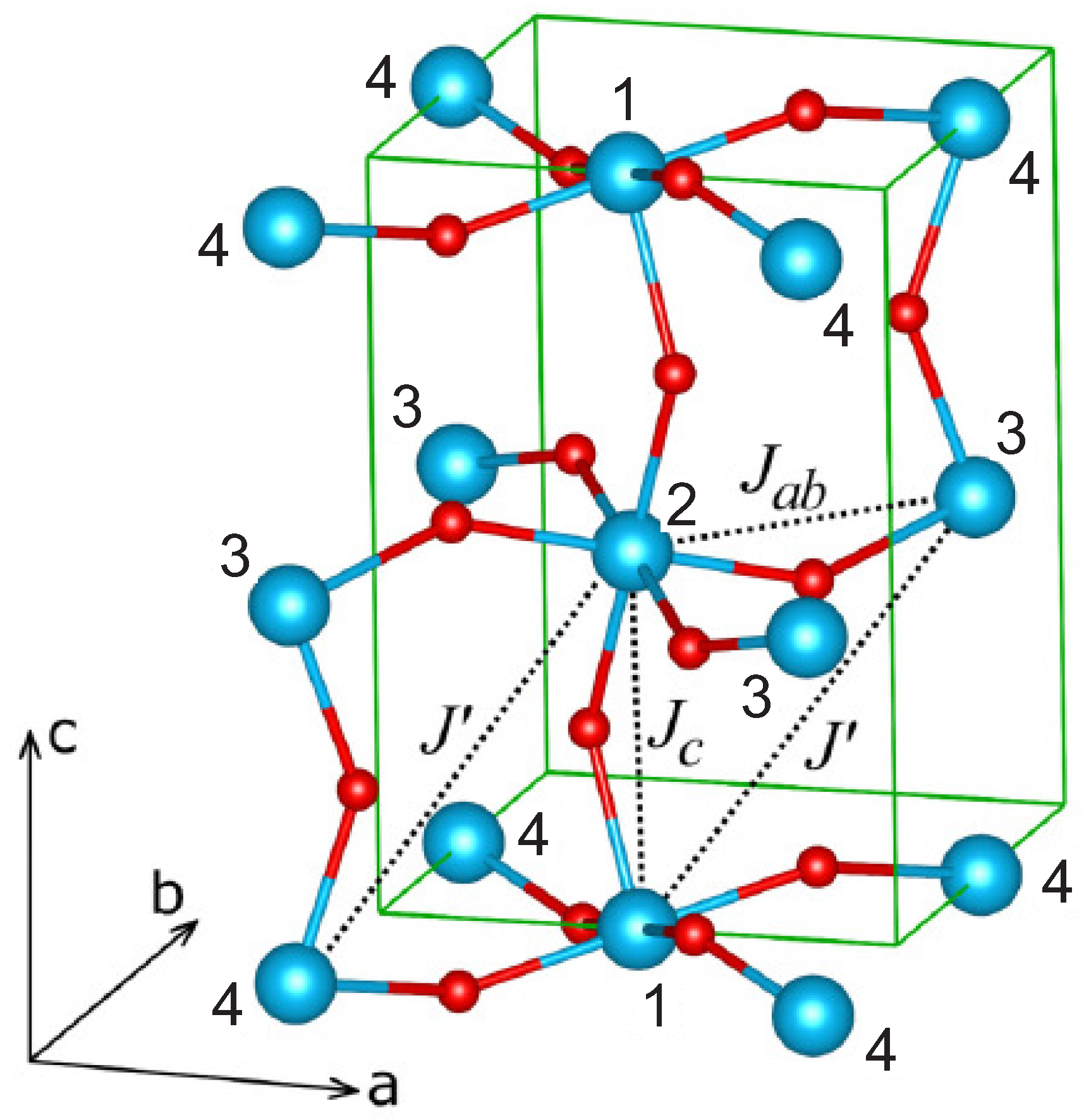
2. Crystal and Magnetic Structure of Rare-Earth Orthoferrites

Orthoferrites are composed of relatively robust corner-shared FeO${}_6$ octahedra, with nominally 12-coordinated rare-earth (R) cations. These adopt low-symmetry distortions from the ideal cubic perovskite Pm$\overline{3}$m symmetry. The Fe atoms are located on inversion centers, the R atom and atom O${}_1$ lie on the mirror planes perpendicular to the orthorhombic b-axis, and atom O${}_2$ occupies a site of general symmetry.

The real FeO${}_6$ complex in orthoferrites can be represented as a homogeneously deformed ideal octahedron. To find the degree of distortion, we introduce a symmetric strain tensor according to the standard rules. In the local system of cubic axes of the octahedron

$${\epsilon }_{ij}=\frac{1}{4l^2}\sum _{n=1}^6(R_i\left(n\right)u_j\left(n\right)+R_j\left(n\right)u_i\left(n\right)),$$

(1)

where R$\left(n\right)$ is the radius-vector of the Fe-O${}_n$ bond, $\mathbf{u}$$\left(n\right)$ is the O${}_n$-ligand displacement vector, or

$$\widehat{\epsilon }=\left(\begin{array}{ccc}1-\frac{l_1}{l}& \frac{1}{2}(\frac{\pi }{2}-{\theta }_{12})& \frac{1}{2}(\frac{\pi }{2}-{\theta }_{13})\\ \frac{1}{2}(\frac{\pi }{2}-{\theta }_{21})& 1-\frac{l_2}{l}& \frac{1}{2}(\frac{\pi }{2}-{\theta }_{23})\\ \frac{1}{2}(\frac{\pi }{2}-{\theta }_{31})& \frac{1}{2}(\frac{\pi }{2}-{\theta }_{32})& 1-\frac{l_3}{l}\end{array}\right),$$

(2)

where l is the Fe-O separation in an ideal octahedron, $l_i$ are the Fe-O${}_i$ interatomic distances $\frac{1}{3}(l_1+l_2+l_3)=l$, and ${\theta }_{ij}$ are the bond angles O${}_i$-Fe-O${}_j$ in a real complex. Local $x,y,z$ axes in the octahedron are defined as follows: the z-axis is directed along the Fe-O${}_I$, the x-axis is along Fe-O${}_{II}$ with the shortest Fe-O bond length. In general, the deformations of octahedra in orthoferrites are small and do not exceed 0.02.

Diagonal components of the traceless strain tensor (2) (tensile/compressive deformations) can be termed E-type deformations since ${\epsilon }_{zz}$ and $\frac{1}{\sqrt{3}}({\epsilon }_{xx}-{\epsilon }_{yy})$ transform according to the irreducible representation (irrep) E of the cubic group O${}_h$, while off-diagonal components (shear deformations) can be termed $T_2$-type deformations since $var{ϵ}_{yz}$, ${\epsilon }_{xz}$, and ${\epsilon }_{xy}$ transform according to the irrep $T_2$ of the cubic group O${}_h$.

The vector $\mathbf{v}$ of rotation of the octahedron FeO${}_6$, the direction and value of which specify the axis and the angle of rotation, respectively, is related to the small displacements of oxygen ions as follows:

$$\mathbf{v}=\frac{1}{4l^2}\sum _{n=1}^6[\mathbf{R}\left(n\right)\times \mathbf{u}\left(n\right)].$$

(3)

Four Fe${}^{3+}$ ions occupy positions 4b in the orthorhombic elementary cell of orthoferrites RFeO${}_3$ (space group $Pbnm$):

$$1(1/2,0,0);2(1/2,0,1/2);3(0,1/2,1/2);4(0,1/2,0).$$

It is worth noting that another labeling of the Fe${}^{3+}$ positions, different to that used here, is found in the literature (see, for example, Refs. [8,9]), in which case the basis vectors $\mathbf{G}$, $\mathbf{C}$, $\mathbf{A}$ may differ in sign.

Classical basis vectors of magnetic structure for 3d sublattice are defined as follows:

$$\begin{array}{c}4S\mathbf{F}={\mathbf{S}}_1+{\mathbf{S}}_2+{\mathbf{S}}_3+{\mathbf{S}}_4;\\ 4S\mathbf{G}={\mathbf{S}}_1-{\mathbf{S}}_2+{\mathbf{S}}_3-{\mathbf{S}}_4;\\ 4S\mathbf{C}={\mathbf{S}}_1+{\mathbf{S}}_2-{\mathbf{S}}_3-{\mathbf{S}}_4;\\ 4S\mathbf{A}={\mathbf{S}}_1-{\mathbf{S}}_2-{\mathbf{S}}_3+{\mathbf{S}}_4,\end{array}$$

(4)

where ${\mathbf{S}}_i$ is classical spin vector for the Fe ion in the i-th position, and S = 5/2 is the spin value. Here, $\mathbf{G}$ describes the main antiferromagnetic component (Néel vector), $\mathbf{F}$ gives the weak ferromagnetic moment (overt canting), the weak antiferromagnetic components $\mathbf{C}$ and $\mathbf{A}$ describe a canting without net magnetic moment (hidden canting). Allowed spin configurations for 3d-sublattice are denoted as ${\Gamma }_1(A_x,G_y,C_z)$, ${\Gamma }_2(F_x,C_y,G_z)$, ${\Gamma }_4(G_x,A_y,F_z)$, where the components given in parentheses are the only ones different from zero. The phase diagram of orthoferrites indicates that all but SmFeO${}_3$ adopt ${\Gamma }_4$ at room temperature.

Competition between the magnetic anisotropy of the Fe sublattice and R-Fe exchange interaction leads to the spin-reorientational transitions ${\Gamma }_4\to {\Gamma }_2$ or ${\Gamma }_1$ depending on R as the temperature decreases [10]. In all cases, the G-component is prevalent: $G\gg F,C,A$.

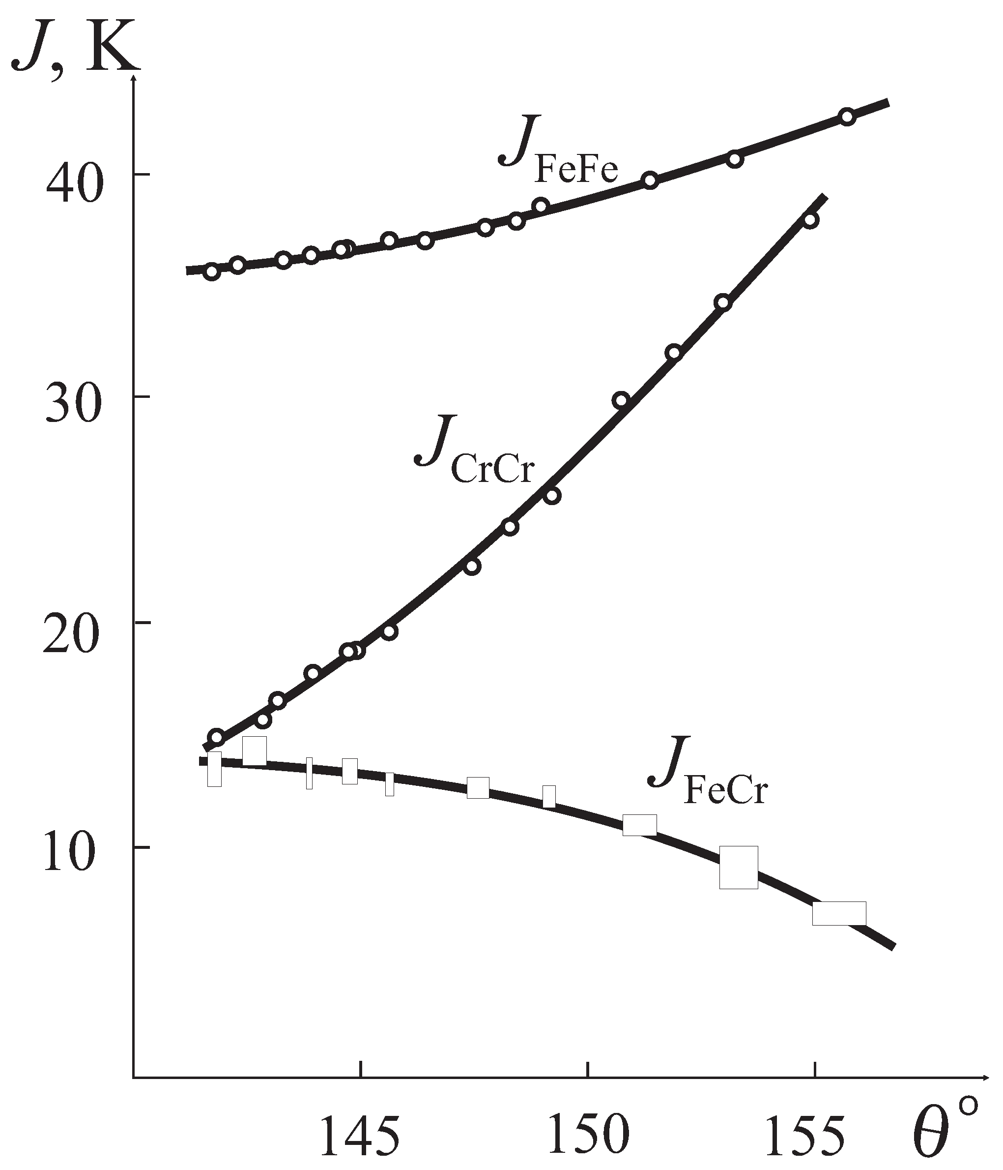
3. Isotropic Superexchange Coupling and Superexchange Geometry

Figure 1 shows the intricate structure of the Fe${}^{3+}$–O${}^{2-}$–Fe${}^{3+}$ superexchange bondings in orthoferrites.

The G-type of the magnetic structure of orthoferrites is determined by the strong isotropic superexchange interaction:

$${\widehat{V}}_{ex}=\sum _{m>n}{J}_{mn}({\mathbf{S}}_m·{\mathbf{S}}_n)$$

(5)

with an exchange integral, which depends primarily on the superexchange Fe-O-Fe bonding angle, which, in turn, is determined by the angles of the rigid rotation of the FeO${}_6$ octahedra, which produce deviations of the Fe-O-Fe bonding angle away from the ideal 180${}^{\circ }$ found in the cubic perovskite aristotype (Pm$\overline{3}$m symmetry).

First poor man’s microscopic derivation for the dependence of the superexchange integral on the bonding angle (see Figure 2) was performed by the author in 1970 [11] under simplified assumptions for S ions with configuration $3d^5$ (Fe${}^{3+}$, Mn${}^{2+}$)

$$J_{12}\left(\theta \right)=a+b·cos{\theta }_{12}+c·{cos}^2{\theta }_{12},$$

(6)

where parameters $a,b,c$ depend on the cation–ligand separation. A more comprehensive analysis has supported the validity of the expression. Interestingly, the second term in (6) is determined by the ligand inter-configurational $2p$-$ns$ excitations, while other terms are related to intra-configurational $2p$-, $2s$- contributions.

Later on, the derivation had been generalized for the $3d$ ions in a strong cubic crystal field (see, e.g., Refs. [4,12,13,14,15,16])

The orbitally isotropic contribution to the superexchange integral for a pair of Fe${}^{3+}$, Cr${}^{3+}$ ions with configurations $t_{2g}^3{e}_g^2$, $t_{2g}^3$, respectively, can be written as follows:

$$\begin{array}{c}{J}_{FeFe}=\frac{1}{25}(4J\left(e_g{e}_g\right)+12J\left(e_g{t}_{2g}\right)+9J\left(t_{2g}{t}_{2g}\right)),\\ J_{CrCr}=J\left(t_{2g}{t}_{2g}\right),\\ J_{FeCr}=\frac{1}{5}(2J\left(e_g{e}_g\right)+3J\left(t_{2g}{t}_{2g}\right)).\end{array}$$

(7)

The kinetic exchange contribution to partial exchange parameters $J\left({\gamma }_i{\gamma }_j\right)$ related to the electron transfer to partially filled shells can be written as follows [12,13]:

$$J\left(e_g{e}_g\right)=\frac{{(t_{ss}+t_{\sigma \sigma }cos\theta )}^2}{2U};J\left(e_g{t}_{2g}\right)=\frac{t_{\sigma \pi }^2}{3U}{sin}^2\theta ;J\left(t_{2g}{t}_{2g}\right)=\frac{2t_{\pi \pi }^2}{9U}(2-{sin}^2\theta ),$$

(8)

where $t_{\sigma \sigma }>t_{\pi \sigma }>t_{\pi \pi }>t_{ss}$ are positive definite $d-d$ transfer integrals, U is a mean $d-d$ transfer energy (correlation energy). All the partial exchange integrals appear to be positive or “antiferromagnetic”, irrespective of the bonding angle value, though the combined effect of the $ss$ and $\sigma \sigma$ bonds $\propto cos\theta$ in $J\left(e_g{e}_g\right)$ yields a ferromagnetic contribution given bonding angles $\pi /2<\theta <\pi$. It should be noted that the “large” ferromagnetic potential contribution [17] has a similar angular dependence [18].

Some predictions regarding the relative magnitude of the $I\left({\gamma }_i{\gamma }_j\right)$ exchange parameters can be made using the relation among different $d-d$ transfer integrals as follows:

$$t_{\sigma \sigma }:t_{\pi \sigma }:t_{\pi \pi }:t_{ss}\approx {\lambda }_{\sigma }^2:{\lambda }_{\pi }{\lambda }_{\sigma }:{\lambda }_{\pi }^2:{\lambda }_s^2,$$

(9)

where ${\lambda }_{\sigma },{\lambda }_{\pi },{\lambda }_s$ are covalency parameters. The simplified kinetic exchange contribution (8) related to the electron transfer to partially filled shells does not account for the intra-center correlations, which are of particular importance for the contribution related to the electron transfer to empty shells. For instance, appropriate contributions related to the transfer to the empty $e_g$ subshell for the Cr${}^{3+}$-Cr${}^{3+}$ and Fe${}^{3+}$-Cr${}^{3+}$ exchange integrals are

$$\Delta J_{CrCr}=-\frac{\Delta E\left(35\right)}{6U}\frac{t_{\sigma \pi }^2}{U}{sin}^2\theta ;\Delta J_{FeCr}=-\frac{\Delta E\left(35\right)}{10U}\left[\frac{{(t_{ss}+t_{\sigma \sigma }cos\theta )}^2}{U}+\frac{t_{\sigma \pi }^2}{U}{sin}^2\theta \right],$$

(10)

where $\Delta E\left(35\right)$ is the energy separation between ${}^3{E}_g$ and ${}^5{E}_g$ terms for $t_{2g}^3{e}_g$ configuration (Cr${}^{2+}$ ion). Obviously, these contributions have a ferromagnetic sign. Furthermore, the exchange integral $J_{CrCr}$ can change sign at $\theta$ = ${\theta }_{cr}$:

$${sin}^2{\theta }_{cr}=\frac{1}{\left(\frac{1}{2}+\frac{3}{8}\frac{\Delta E\left(35\right)}{U}\frac{t_{\sigma \pi }^2}{t_{\pi \pi }^2}\right)}.$$

(11)

The microscopically derived angular dependence of the superexchange integrals describes the experimental data for exchange integrals $J_{FeFe}$, $J_{CrCr}$, and $J_{FeCr}$ in orthoferrites, orthochromites, and orthoferrites–orthochromites [14] (see Figure 3). The fitting allows us to predict the sign change for $J_{CrCr}$ and $J_{FeCr}$ at ${\theta }_{12}$ ≈ 133${}^{\circ }$ and 170${}^{\circ }$, respectively. In other words, the Cr${}^{3+}$-O${}^{2-}$-Cr${}^{3+}$ (Fe${}^{3+}$-O${}^{2-}$-Cr${}^{3+}$) superexchange coupling becomes ferromagnetic at ${\theta }_{12}\le {133}^{\circ }$ (${\theta }_{12}\ge {170}^{\circ }$). However, it should be noted that the overly narrow (141–156${}^{\circ }$) range of the superexchange bonding angles that we used for the fitting with the assumption of the same Fe(Cr)-O bond separations and mean superexchange bonding angles for all the systems gives rise to a sizeable parameter’s uncertainty, particularly for $J_{FeFe}$ and $J_{FeCr}$. In addition, it is necessary to note the large uncertainty regarding what is here called the “experimental” value of the exchange integral. The fact is that the “experimental” exchange integrals that we have just used above are calculated using a simple MFA relation for the Néel temperature:

$$T_N=\frac{zS(S+1)}{3k_B}J,$$

(12)

however, this relation yields the exchange integrals that can be one and a half or even two times lower than the values obtained by other methods [12,19].

Above, we addressed only the typically antiferromagnetic kinetic (super)exchange contribution as a result of the second-order perturbation theory. However, this contribution does in fact compete with the typically ferromagnetic potential (super)exchange contribution, or Heisenberg exchange, which is a result of the first-order perturbation theory. The most important contribution to the potential superexchange can be related to the intra-atomic ferromagnetic Hund exchange interaction of unpaired electrons on orthogonal ligand orbitals hybridized with the $3d$-orbitals of the two nearest magnetic cations.

The strong dependence of the $d-d$ superexchange integrals on the cation–ligand–cation separation is usually described by the Bloch’s rule [20]:

$$\frac{\partial lnJ}{\partial lnR}=\frac{\partial J}{\partial R}/\frac{J}{R}\approx -10.$$

(13)

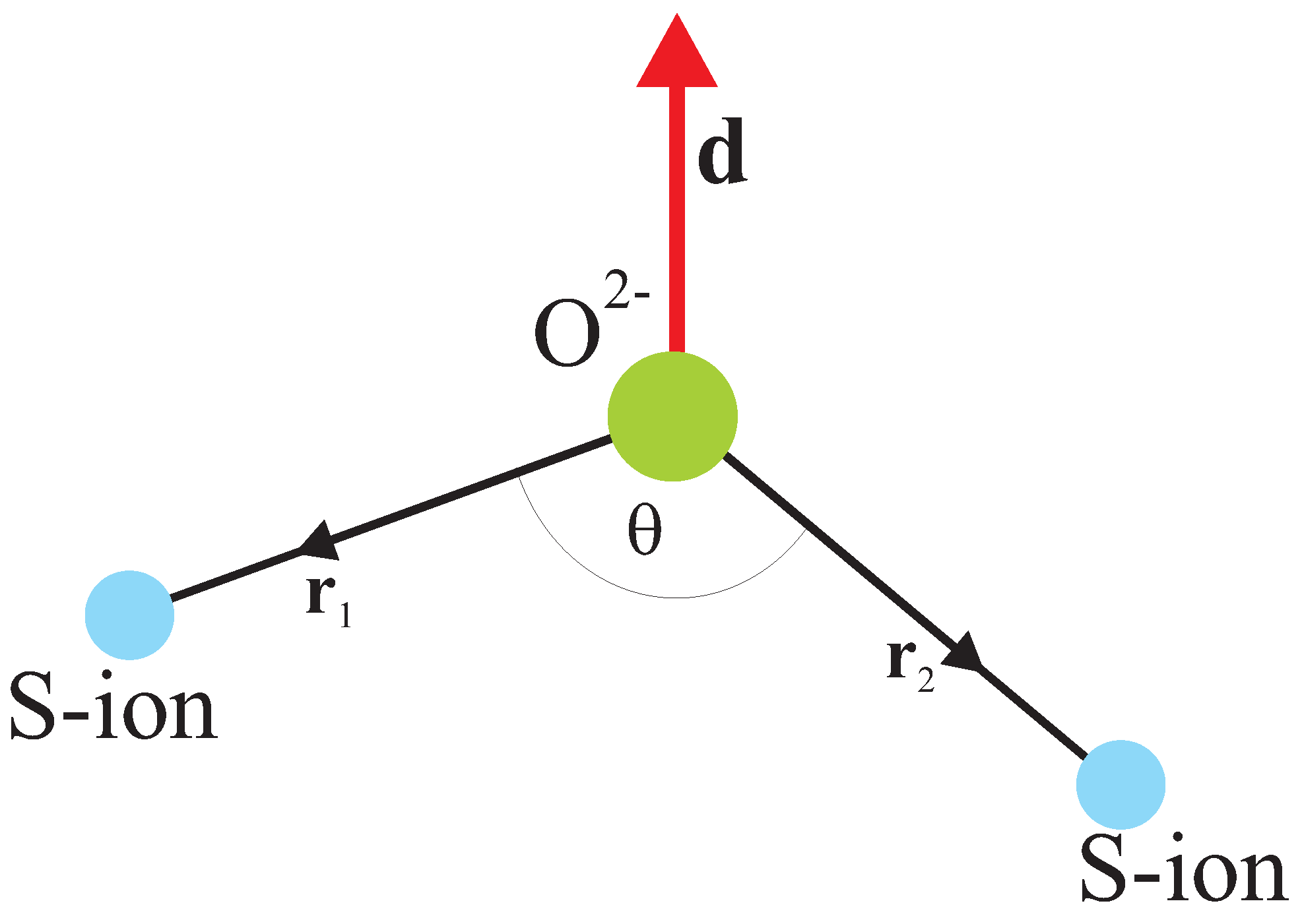
4. Crystal Structure and the DM Coupling in Orthoferrites

Weak ferromagnetism is one of the most remarkable physical properties of orthoferrites. A theoretical explanation and first thermodynamic theory for weak ferromagnetism was provided by I. E. Dzyaloshinskii [21,22] in 1957 on the basis of symmetry considerations and Landau’s theory of phase transitions of the second kind.

The free energy of a two-sublattice uniaxial weak ferromagnet such as $\alpha$-Fe${}_2$O${}_3$, MnCO${}_3$, CoCO${}_3$, FeBO${}_3$ was shown to be written as follows:

$$\begin{array}{c}F=M{H}_E({\mathbf{m}}_1·{\mathbf{m}}_2)-M{\mathbf{H}}_0({\mathbf{m}}_1+{\mathbf{m}}_2)+E_D+E_A\\ =M{H}_E({\mathbf{m}}^2-{\mathbf{l}}^2)-M{\mathbf{H}}_0\mathbf{m}+E_D+E_A.\end{array}$$

(14)

In this expression, ${\mathbf{m}}_1$ and ${\mathbf{m}}_2$ are unit vectors in the directions of the sublattice moments, M is the sublattice magnetization, $\mathbf{m}=\frac{1}{2}({\mathbf{m}}_1+{\mathbf{m}}_2)$ and $\mathbf{l}=\frac{1}{2}({\mathbf{m}}_1-{\mathbf{m}}_2)$ are the ferro- and antiferromagnetic vectors, respectively, $H_0$ is the applied field, $H_E$ is the exchange field,

$$\begin{array}{c}{E}_D=-M{H}_D{[{\mathbf{m}}_1\times {\mathbf{m}}_2]}_z=+2M{H}_D{[\mathbf{m}\times \mathbf{l}]}_z=\\ +2M{H}_D(m_x{l}_y-m_y{l}_x)\end{array}$$

(15)

is now called the Dzyaloshinskii interaction, $H_D$ > 0 is the Dzyaloshinskii field. The anisotropy energy $E_A$ is assumed to have the form: $E_A=H_A/2M(m_{1z}^2+m_{2z}^2)=2H_A/2M(m_z^2+l_z^2)$, where $H_A$ is the anisotropy field. The choice of sign for the anisotropy field $H_A$ assumes that the c axis is a hard direction of magnetization. In a general sense, the Dzyaloshinskii interaction implies the terms that are linear both on ferro- and antiferromagnetic vectors. For instance, in orthorhombic orthoferrites and orthochromites, the Dzyaloshinskii interaction consists of the antisymmetric and symmetric terms

$$\begin{array}{c}{E}_D=d_1{m}_z{l}_x+d_2{m}_x{l}_z=\\ \frac{d_1-d_2}{2}(m_z{l}_x-m_x{l}_z)+\frac{d_1+d_2}{2}(m_z{l}_x+m_x{l}_z)=\\ -2M{H}_D{[\mathbf{m}\times \mathbf{l}]}_y+\frac{d_1+d_2}{2}(m_z{l}_x+m_x{l}_z),\end{array}$$

(16)

while for tetragonal fluorides NiF${}_2$ and CoF${}_2$, the Dzyaloshinskii interaction consists of the only symmetric term. Although Dzyaloshinskii supposed that weak ferromagnetism is due to the relativistic spin-lattice and magnetic dipole interaction, the theory was a phenomenological one and did not clarify the microscopic nature of the Dzyaloshinskii interaction that does result in the canting.

Later on, in 1960, T. Moriya [23,24] suggested a model microscopic theory of the exchange-relativistic antisymmetric exchange interaction to be the main contributing mechanism of weak ferromagnetism. He extended the Anderson theory of superexchange to include spin-orbital coupling $V_{so}={\sum }_i\xi ({\mathbf{l}}_i·{\mathbf{s}}_i)$, where $\xi$ is the coupling constant, and derived a spin-Hamiltonian

$$V_{DM}=\sum _{mn}({\mathbf{d}}_{mn}·\left[{\mathbf{S}}_m\times {\mathbf{S}}_n\right]),$$

(17)

now called Dzyaloshinskii–Moriya (DM) spin coupling. Here, ${\mathbf{d}}_{mn}$ is the axial Dzyaloshinskii vector.

Moriya found the symmetry constraints on the orientation of the Dzyaloshinskii vector ${\mathbf{d}}_{ij}$. Two ions 1 and 2 are located at the points A and B, respectively, with C point bisecting the AB line:

• When C is a center of inversion: d = 0.
• When a mirror plane ⊥AB passes through C, $\mathbf{d}\Vert$ mirror plane or $\mathbf{d}\perp$ AB.
• When there is a mirror plane including A and B, $\mathbf{d}\perp$ mirror plane.
• When a twofold rotation axis ⊥ AB passes through C, $\mathbf{d}\perp$ twofold axis.
• When there is an n-fold axis (n ≥ 2) along AB, $\mathbf{d}\Vert$ AB.

Recently, Keffer [25] proposed a simple phenomenological expression for the Dzyaloshinskii vector for two magnetic ions M${}_i$ and M${}_j$ interacting by the superexchange mechanism via intermediate ligand O (see Figure 2):

$${\mathbf{d}}_{ij}\propto [{\mathbf{r}}_i\times {\mathbf{r}}_j],$$

(18)

where ${\mathbf{r}}_{i,j}$ are unit radius vectors for O − M${}_{i,j}$ bonds with presumably equal bond lengths. Later on, Moskvin [11] derived a microscopic formula for the Dzyaloshinskii vector in a pair of the S-type ions

$${\mathbf{d}}_{ij}=d_{ij}\left(\theta \right)[{\mathbf{r}}_i\times {\mathbf{r}}_j],$$

(19)

where

$$d_{ij}\left(\theta \right)=d_1(R_i,R_j)+d_2(R_i,R_j)cos{\theta }_{ij}.$$

(20)

In other words, at variance with the superexchange integral, the Dzyaloshinskii vector depends both on the superexchange bonding angle and spatial Fe–O–Fe bond orientation.

Note that the relation $d/J\approx \Delta g/g$, where g is the gyromagnetic ratio and $\Delta g$ is its deviation from the free-electron value, proposed by Moriya for estimating the magnitude of the Dzyaloshinskii vector, should be used with extreme caution. Therefore, in the case of S-ions such as Fe${}^{3+}$, Mn${}^{2+}$, it is simply inapplicable.

The spin nondiagonality of the DM coupling implies very unusual features of the $\mathbf{d}$-vector somewhat resembling a vector orbital operator whose transformational properties cannot be isolated from the lattice. It seems that the $\mathbf{d}$-vector does not transform as a vector at all.

Within the simplest classical approximation the operator of symmetric and antisymmetric d − d exchange interactions in orthoferrites

$$\widehat{H}=\sum _{i>j}{J}_{ij}({\mathbf{S}}_i·{\mathbf{S}}_j)+\sum _{i>j}({\mathbf{d}}_{ij}·[{\mathbf{S}}_i\times {\mathbf{S}}_j])$$

(21)

can be written in terms of basis vectors as a free energy (see, e.g., Refs. [12,16,26] and references therein). Neglecting the terms quadratic in the components of small basis vectors $\mathbf{F}$, $\mathbf{C}$, $\mathbf{A}$, we obtain for the free energy per ion

$$\begin{array}{c}\Phi =\frac{J_F}{2}{\mathbf{F}}^2+\frac{J_G}{2}{\mathbf{G}}^2+\frac{J_C}{2}{\mathbf{C}}^2+\frac{J_A}{2}{\mathbf{A}}^2+\\ D_x(C_y{G}_z-C_z{G}_y)+D_y(F_z{G}_x-F_x{G}_z)+D_z(A_x{G}_y-A_y{G}_x),\end{array}$$

(22)

where

$$\begin{array}{c}{J}_F=-J_G=S^2(2J_{ab}+J_c);J_A=-J_C=S^2(2J_{ab}-J_c);\\ D_x=-S^2{\displaystyle \sum _2}{d}_x\left(12\right);\\ D_y=-S^2\left({\displaystyle \sum _4}{d}_y\left(14\right)+{\displaystyle \sum _2}{d}_y\left(12\right)\right);\\ D_z=-S^2{\displaystyle \sum _4}{d}_z\left(14\right),\end{array}$$

(23)

where $J_{ab}$ and $J_c$ are Fe-Fe exchange integrals in the $ab$ plane and along the c axis, respectively (see Figure 1), and $d_{x,y,z}\left(ij\right)$ are the components of the Dzyaloshinskii vector for the Fe${}_i$-Fe${}_j$ bond. By minimizing the free energy under condition ${\mathbf{F}}^2+{\mathbf{G}}^2+{\mathbf{C}}^2+{\mathbf{A}}^2=1$ and $F,C,A\ll G$, we find

$$\begin{array}{c}{F}_z=-\frac{D_y}{J_F-J_G}{G}_x;A_y=\frac{D_z}{J_A-J_G}{G}_x;\\ F_x=\frac{D_y}{J_F-J_G}{G}_z;C_y=-\frac{D_x}{J_C-J_G}{G}_z;\\ A_x=-\frac{D_z}{J_A-J_G}{G}_y;C_z=\frac{D_x}{J_C-J_G}{G}_y;\end{array}$$

(24)

The relative orientation of the basis vectors for different signs of the Dzyaloshinskii vector is shown in Figure 4.

Hereafter, we address the DM coupling for the S-type magnetic $3d$ ions with orbitally nondegenerate high-spin ground state in a strong cubic crystal field—that is, for the $3d$ ions with half-filled shells $t_{2g}^3$, $t_{2g}^3{e}_g^2$, $t_{2g}^6{e}_g^2$ and ground states ${}^4{A}_{2g}$, ${}^6{A}_{1g}$, ${}^3{A}_{2g}$, respectively. The strong crystal field approximation seems to be more appropriate for the most part of $3d$ ions in crystals.

Making use of expressions for spin-orbital coupling $V_{so}$ and the main kinetic contribution to the superexchange parameters, which define the DM coupling, after routine algebra, we have found that the DM coupling can be written in a standard form (17) with the Dzyaloshinskii vector (19), where $d_{12}$ can be written as follows [4,12,15,16,27]:

$$d_{12}=X_1{Y}_2+X_2{Y}_1,$$

(25)

where the exchange factors X and dimensionless spin-orbital factors Y do reflect the exchange-relativistic structure of the second-order perturbation theory and details of the electron configurations for S-type ions.

The factors X and Y are presented in

Table 1. Expressions for the X and Y parameters that define the magnitude and the sign of the Dzyaloshinskii vector in pairs of the S-type 3d ions with local octahedral symmetry. Signs for $X_i$ correspond to the bonding angle $\theta >{\theta }_{cr}$.

Ground State Configuration	X	Sign X	Y	Sign Y	Excited State Configuration
$3d^3$($t_{2g}^3$):${}^4{A}_{2g}$ $V^{2+}$, $C{r}^{3+}$, $M{n}^{4+}$	$-\frac{1}{3U}{t}_{\pi \pi }{t}_{\sigma \pi }cos\theta$	+	$\frac{2{\xi }_{3d}}{3\sqrt{3}}(\frac{1}{\Delta E_{{}^4{T}_{2g}}}+\frac{2}{\Delta E_{{}^2{T}_{2g}}})$	+	$t_{2g}^2{e}_g^1$
$3d^5$($t_{2g}^3{e}_g^2$):${}^6{A}_{1g}$ $M{n}^{2+}$, $F{e}^{3+}$	$-\frac{1}{5U}(t_{\pi \pi }{t}_{\sigma \pi }cos\theta$− $t_{\pi \sigma }\left(t_{ss}+t_{\sigma \sigma }cos\theta )\right)$	−	$-\frac{6{\xi }_{3d}}{5\sqrt{3}}(\frac{1}{\Delta E_{{}^4{T}_{1g}}\left(41\right)}-\frac{1}{\Delta E_{{}^4{T}_{1g}}\left(23\right)})$	−	$t_{2g}^4{e}_g^1$, $t_{2g}^2{e}_g^3$
$3d^8$($t_{2g}^6{e}_g^2$):${}^3{A}_{2g}$ $N{i}^{2+}$, $C{u}^{3+}$	$\frac{1}{2U}{t}_{\pi \sigma }(t_{ss}+t_{\sigma \sigma }cos\theta )$	−	$\frac{3{\xi }_{3d}}{2\sqrt{3}}(\frac{1}{\Delta E_{{}^3{T}_{2g}}}+\frac{1}{\Delta E_{{}^1{T}_{2g}}})$	+	$t_{2g}^5{e}_g^3$

for S-type 3d-ions. There, ${\xi }_{3d}$ is the spin-orbital parameter, $\Delta E_{{}^{2S+1}\Gamma }$ is the energy of the ${}^{2S+1}\Gamma$ crystal term, $t_{\sigma \sigma }>t_{\pi \sigma }>t_{\pi \pi }>t_{ss}$ are positive definite d-d transfer integrals, U is the d-d transfer energy (correlation energy).

Note that the value of the Dzyaloshinskii vector in our approximation depends on the parameters of the FeO${}_6$ octahedra rotation and does not depend at all on octahedral distortions, or on the parameters of the low-symmetry crystal field for Fe centers, and hence on the $\delta g$ values, characterizing the deviation of the g- factor from its value in a free ion. Moriya’s estimation $d/J\approx \Delta g/g$ in this case does not work at all. In particular, the authors of Ref. [7] incorrectly associate the value of $\delta \widehat{g}=2\lambda \widehat{\Lambda }$ (see expression (3) there) with the spin canting angle for orthoferrites.

The signs for X and Y factors in Table 1 are predicted for rather large superexchange bonding angles $|cos{\theta }_{12}|>t_{ss}/t_{\sigma \sigma }$, which are typical for many $3d$ compounds such as oxides, and a relation $\Delta E_{{}^4{T}_{1g}}\left(41\right)<\Delta E_{{}^4{T}_{1g}}\left(32\right)$, which is typical for high-spin $3d^5$ configurations.

On the whole, the data in Table 1 allow us to evaluate both the numerical value and sign of the $d_{12}$ parameters.

It should be noted that for critical angle ${\theta }_{cr}$, when the Dzyaloshinskii vector changes its sign, we have $cos{\theta }_{cr}=-d_1/d_2=\frac{{\lambda }_s^2}{{\lambda }_{\sigma }^2}$ for $d^8-d^8$ pairs and $cos{\theta }_{cr}=-d_1/d_2=\frac{{\lambda }_s^2}{{\lambda }_{\sigma }^2-{\lambda }_{\pi }^2}$ for $d^5-d^5$ pairs. Making use of different experimental data for covalency parameters (see, e.g., Ref. [28]), we arrive at $d_1/d_2\sim \frac{1}{5}-\frac{1}{3}$ and ${\theta }_{cr}\approx {100}^{\circ }-{110}^{\circ }$ for Fe${}^{3+}$-Fe${}^{3+}$ pairs in oxides.

The relation among different Xs given the superexchange geometry and covalency parameters typical for orthoferrites and orthochromites [12] is

$$|X_{d^8}|\ge |X_{d^3}|\ge |X_{d^5}|,$$

(26)

however, its sensitivity both to superexchange geometry and covalency parameters should be noted. A simple comparison of the exchange parameters X (see Table 1) with exchange parameters $I\left({\gamma }_i{\gamma }_j\right)$ (8) evidences their close magnitudes. Furthermore, the relation (9) allows us to maintain more definite correspondence.

Theoretically predicted signs of the Dzyaloshinskii vector in pairs of the S-type 3d ions with local octahedral symmetry (the sign rules) are presented in

Table 2. Sign rules for the Dzyaloshinskii vector in pairs of the S-type 3d ions with local octahedral symmetry and the bonding angle $\theta >{\theta }_{cr}$.

$3{\mathit{d}}^{\mathit{n}}$	$3{\mathit{d}}^3$(${\mathit{t}}_{2\mathit{g}}^3$)	$3{\mathit{d}}^5$(${\mathit{t}}_{2\mathit{g}}^3{\mathit{e}}_{\mathit{g}}^2$)	$3{\mathit{d}}^8$(${\mathit{t}}_{2\mathit{g}}^6{\mathit{e}}_{\mathit{g}}^2$)
$3d^3$($t_{2g}^3$)	+	−	+
$3d^5$($t_{2g}^3{e}_g^2$)	−	+	+
$3d^8$($t_{2g}^6{e}_g^2$)	+	+	−

. The signs for $d^3-d^3$, $d^5-d^5$, and $d^3-d^8$ pairs turn out to be the same but opposite to the signs for $d^3-d^5$ and $d^8-d^8$ pairs. Similar to the way in which different signs of the conventional exchange integral determine different (ferro-antiferro) magnetic orders, the different signs of the Dzyaloshinskii vectors create the possibility of nonuniform (ferro-antiferro) ordering of local weak (anti)ferromagnetic moments, or local overt/hidden cantings. Novel magnetic phenomenon and a novel class of magnetic materials, which are systems such as solid solutions YFe${}_{1-x}$Cr${}_x$O${}_3$ with competing signs of the Dzyaloshinskii vectors, are discussed in Refs. [4,15,16,29] in more detail.

At variance with isotropic superexchange coupling, the DM coupling has a much more complicated structural dependence. Figure 1 shows the intricate structure of the Fe${}^{3+}$–O${}^{2-}$–Fe${}^{3+}$ superexchange bondings in orthoferrites that points to a complicated structural dependence of the Dzyaloshinskii vectors.

In

Table 3. The structural factors ${\left[{\mathbf{r}}_1\times {\mathbf{r}}_2\right]}_{x,y,z}$ for the superexchange coupled Fe-O-Fe pairs in orthoferrites with numerical values for YFeO${}_3$. See text for details.

	${\left[{\mathit{r}}_1\times {\mathit{r}}_2\right]}_{\mathit{x}}$	${\left[{\mathit{r}}_1\times {\mathit{r}}_2\right]}_{\mathit{y}}$	${\left[{\mathit{r}}_1\times {\mathit{r}}_2\right]}_{\mathit{z}}$
1a	$-\frac{z_{2}bc}{2l^2}$ = −0.31	$-\frac{z_{2}ac}{2l^2}$ = −0.29	$\frac{(y_2-x_2+\frac{1}{2})ab}{2l^2}$ = 0.41
1b	$+\frac{z_{2}bc}{2l^2}$ = 0.31	$-\frac{z_{2}ac}{2l^2}$ = −0.29	$\frac{(y_2-x_2+\frac{1}{2})ab}{2l^2}$ = 0.41
3a	$\frac{(\frac{1}{2}-y_1)bc}{2l^2}$ = 0.20	$-\frac{x_{1}ac}{2l^2}$ = −0.55	0

, we present structural factors ${\left[{\mathbf{r}}_1\times {\mathbf{r}}_2\right]}_{x,y,z}$ for the superexchange coupled Fe-O-Fe pairs in orthoferrites with numerical values for YFeO${}_3$ [30,31]. In all cases, the vector ${\mathbf{r}}_1$ is oriented to the Fe ion in the position (1/2,0,0), and the vectors ${\mathbf{r}}_2$ are oriented to the nearest Fe ions in the $ab$ plane (1a, 1b) or along the c axis (3a). It is easy to see that the weak ferromagnetism in orthoferrites governed by the y component of the Dzyaloshinskii vector actually makes use of only around one-third of its maximal value.

A simple formula for the Dzyaloshinskii vector (19) and structural factors from Table 3 can be used to find a relation between crystallographic and canted magnetic structures for four-sublattice orthoferrites RFeO${}_3$ and orthochromites RCrO${}_3$ [4,12,15,16,32] (see Figure 4), where the main G-type antiferromagnetic order is accompanied by both overt canting characterized by ferromagnetic vector $\mathbf{F}$ (weak ferromagnetism!) and two types of a hidden canting, $\mathbf{A}$ and $\mathbf{C}$ (weak antiferromagnetism!):

$$\begin{array}{c}{F}_z=\frac{(x_1+2z_2)ac}{6l^2}\frac{d}{J}{G}_x;F_x=-\frac{(x_1+2z_2)ac}{6l^2}\frac{d}{J}{G}_z;A_y=\frac{(\frac{1}{2}+y_2-x_2)ab}{2l^2}\frac{d}{J}{G}_x;\\ A_x=-\frac{(\frac{1}{2}+y_2-x_2)ab}{2l^2}\frac{d}{J}{G}_y;C_y=\frac{(\frac{1}{2}-y_1)bc}{2l^2}\frac{d}{J}{G}_z;C_z=-\frac{(\frac{1}{2}-y_1)bc}{2l^2}\frac{d}{J}{G}_y,\end{array}$$

(27)

where $a,b,c$ are unit cell parameters, $x_{1,2},y_{1,2},z_2$ are oxygen ($O_{I,II}$) parameters [30], l is a mean cation–anion separation. These relations imply an averaging on the Fe${}^{3+}$-O${}^{2-}$-Fe${}^{3+}$ bonds in the $ab$ plane and along the c axis. It is worth noting that $|A_{x,y}|>|F_{x,z}|>|C_{y,z}|$.

First of all, we arrive at a simple relation between the crystallographic parameters, canting angle, and magnetic moment of the Fe sublattice: in units of $G·g/c{m}^3$

$$M_{Fe}=\frac{4g_S{\beta }_{e}S}{\rho V}\left|F_{x,z}\right|=\frac{2g{\beta }_{e}Sac}{3l^2\rho V}(x_1+2z_2)\frac{d\left(\theta \right)}{J\left(\theta \right)},$$

(28)

where $\rho$ and V are the unit cell density and volume, respectively.

The theoretically predicted value of the spin canting angle along the c axis, or $F_z$ component, increases monotonically from LaFeO${}_3$ to LuFeO${}_3$ (see Figure 5), which is in excellent agreement with the latest experimental data obtained on precisely oriented crystals of orthoferrites with a nonmagnetic R ion, R = La, Y, Lu [7]). The authors of Ref. [7] erroneously interpreted this dependence as evidence that “...single-ion anisotropy effect is responsible for the spin canting in the type-G antiferromagnets orthoferrites”.

The overt canting $F_{x,z}$ can be calculated through the ratio of the Dzyaloshinskii ($H_D$) and exchange ($H_E$) fields as follows:

$$F=H_D/2H_E.$$

(29)

If we know the Dzyaloshinskii field, we can calculate the $d\left(\theta \right)$ parameter in orthoferrites as follows:

$$H_D=\frac{S}{g{\mu }_B}\sum _i|d_y\left(1i\right)|=\frac{S}{g{\mu }_B}(x_1+2z_2)\frac{ac}{l^2}\left|d\left(\theta \right)\right|,$$

(30)

which yields $\left|d\right(\theta \left)\right|\cong$ 3.2 K in YFeO${}_3$ given $H_D$ = 140 kOe [33]. It is worth noting that despite $F_z\approx$ 0.01, the $d\left(\theta \right)$ parameter is only one order of magnitude smaller than the exchange integral in YFeO${}_3$.

Our results have stimulated experimental studies of the hidden canting, or “weak antiferromagnetism”, in orthoferrites. As shown in

Table 4. Hidden canting in orthoferrites.

Orthoferrite	A${}_{\mathit{y}}$/F${}_{\mathit{z}}$, Theory [32]	A${}_{\mathit{y}}$/F${}_{\mathit{z}}$, exp	A${}_{\mathit{y}}$/C${}_{\mathit{y}}$, Theory [32]	A${}_{\mathit{y}}$/C${}_{\mathit{y}}$, exp
YFeO${}_3$	1.10	1.10 ± 0.03 [34] 1.4 ± 0.2 [35] 1.1 ± 0.1 [38]	2.04	?
HoFeO${}_3$	1.16	0.85 ± 0.10 [38]	2.00	?
TmFeO${}_3$	1.10	1.25 ± 0.05 [34]	1.83	?
YbFeO${}_3$	1.11	1.22 ± 0.05 [35]	1.79	2.0 ± 0.2 [34]

, the theoretically predicted relations between overt and hidden canting agree well with the experimental data obtained for different orthoferrites by NMR [34] and neutron diffraction [35,36,37,38].

In all cases, the magnitude of the Dzyaloshinskii vector ${\mathbf{d}}_{12}$ is anticorrelated with the magnitude of the superexchange integral $J_{12}$ in the sense that the superexchange geometry, favorable for the former, is unfavorable for the latter. The specific supersensitivity of the DM coupling to the superexchange geometry allows us to consider this interaction—first of all, the value and orientation of the Dzyaloshinskii vector—as one of the most important indicators determining the role of structural factors.

Determination of the “sign” of the Dzyloshinskii vector is of fundamental importance from the standpoint of the microscopic theory of the DM coupling. As was first shown in our paper [39], reliable local information on the sign of the Dzyaloshinskii vector, or, to be exact, that of the scalar Dzyaloshinskii parameter $d_{12}$, can be extracted from the ligand NMR data in weak ferromagnets. The procedure was described in detail for ${}^{19}$F NMR data in a weak ferromagnet FeF${}_3$ [39]. The theoretically simulated NMR spectrum agrees well with the experimental ones only for the “right” mutual orientations of the $\mathbf{F}$ and $\mathbf{G}$ vectors, which means $d\left(FeFe\right)>0$ in full accordance with our theoretical sign predictions (see Table 2). The same result, $d\left(FeFe\right)>0$, follows from the the magnetic x-ray scattering amplitude measurements in the weak ferromagnet FeBO${}_3$ [40].

The DM Coupling and Effective Magnetic Anisotropy

At variance with the spin-symmetric single-ion anisotropy and anisotropic exchange, the Dzyaloshinskii–Moriya interaction is a source of spin-antisymmetric anisotropy. Hereafter, we demonstrate a contribution of the DM coupling to effective magnetic anisotropy in orthoferrites within a simple classical approach. Taking into account the expression (22) for the classical energy of orthoferrite and relations (24) for small basis vectors, the classical energies of the three spin configurations ${\Gamma }_1(A_x,G_y,C_z)$, ${\Gamma }_2(F_x,C_y,G_z)$, and ${\Gamma }_4(G_x,A_y,F_z)$ given $|F_x|=|F_z|=F$, $|C_y|=|C_z|=C$, $|A_x|=|A_z|=A$ can be written as follows [4,12,16]:

$$\begin{array}{c}\hfill E_{{\Gamma }_1}=J_G-48J{S}^2{F}^2\left[\frac{1}{3}{\left(\frac{C}{F}\right)}^2+\frac{2}{3}{\left(\frac{A}{F}\right)}^2\right];\end{array}$$

(31)

$$\begin{array}{c}\hfill E_{{\Gamma }_2}=J_G-48J{S}^2{F}^2\left[1+\frac{1}{3}{\left(\frac{C}{F}\right)}^2\right];\end{array}$$

(32)

$$\begin{array}{c}\hfill E_{{\Gamma }_4}=J_G-48J{S}^2{F}^2\left[1+\frac{2}{3}{\left(\frac{A}{F}\right)}^2\right],\end{array}$$

(33)

with the obvious relation $E_{{\Gamma }_4}<E_{{\Gamma }_1}\le E_{{\Gamma }_2}$. The energies allow us to find the constants of the in-plane magnetic anisotropy $E_{an}=k_{1}cos2\theta$ ($ac$, $bc$ planes, $\theta$ is the polar angle of the $\mathbf{G}$ vector), $E_{an}=k_{1}cos2\phi$ ($ab$ plane, $\phi$ is the azimutal angle of the $\mathbf{G}$ vector): $k_1\left(ac\right)=\frac{1}{2}(E_{{\Gamma }_2}-E_{{\Gamma }_4})$; $k_1\left(bc\right)=\frac{1}{2}(E_{{\Gamma }_2}-E_{{\Gamma }_1})$; $k_1\left(ab\right)=\frac{1}{2}(E_{{\Gamma }_4}-E_{{\Gamma }_1})$. Detailed analysis of different mechanisms of the magnetic anisotropy of the orthoferrites [4,12,16] points to a leading contribution of the DM coupling. Indeed, for all the orthoferrites RFeO${}_3$, this mechanism does predict a minimal energy for the ${\Gamma }_4$ configuration, which is actually realized as a ground state for all the orthoferrites, if one neglects the R-Fe interaction. Furthermore, the predicted value of the constant of the magnetic anisotropy in the $ac$ plane for YFeO${}_3$ $k_1\left(ac\right)$ =2.0$\times {10}^5$ erg/cm${}^3$ is close enough to the experimental value of 2.5$\times {10}^5$ erg/cm${}^3$ [33]. Interestingly, the model predicts a close energy for ${\Gamma }_1$ and ${\Gamma }_2$ configurations so that $|k_1\left(bc\right)|$ is around one order of magnitude less than $|k_1\left(ac\right)|$ and $|k_1\left(ab\right)|$ for most orthoferrites [4,12,16]. This means that the anisotropy in the $bc$ plane will be determined by a competition of the DM coupling with relatively weak contributors such as magneto-dipole interaction and single-ion anisotropy. It should be noted that the sign and value of the $k_1\left(bc\right)$ is of great importance for the determination of the type of the domain walls for orthoferrites in their basic ${\Gamma }_4$ configuration (see, e.g., Ref. [41]).

In conclusion, we emphasize once again that we are considering the classical theory of the magnetic state of orthoferrites, which is the result of a simple MFA approximation. The applicability of this popular approximation to the description of quantum antiferromagnets with the Dzyaloshinskii interaction, particularly the anisotropy effects, raises natural doubts. For example, in the author’s paper [42], the role of the DM interaction as a source of magnetic anisotropy is considered in detail and it is shown that for quantum s = 1/2 antiferromagnets in contrast to the simple MFA approach, the DM contribution to the energy of anisotropy for an exchange-coupled spin-1/2 pair becomes zero. However, just as in the case of isotropic exchange, the use of the classical description of the DM interaction for magnets with a large spin S = 5/2 seems quite reasonable.

5. Magnetic and Magnetoelastic Anisotropy in Orthoferrites

5.1. Second-Order Spin Anisotropy

The free energy of the second-order spin anisotropy of the Fe sublattice in orthoferrites can be written as follows [12,26]:

$${\Phi }_{an}^{\left(2\right)}=D{G}_z^2+E(G_x^2-G_y^2)+2p(G_x{A}_y+G_y{A}_x)+2q(G_y{C}_z+G_z{C}_y)+2r(G_x{F}_z+G_z{F}_x),$$

(34)

where we confine ourselves to terms that are linear and quadratic in the components of the main antiferromagnetic vector $\mathbf{G}$. First, let us pay attention to the appearance of three terms of the type of symmetric Dzyaloshinskii interaction, the inclusion of which leads to “symmetric” corrections in the expressions for the parameters of the overt and hidden canting (24) and (27). In particular, taking into account that the r-contribution leads to the appearance of a difference between the $F_x$ and $F_z$ weak ferromagnetic components:

$$\frac{F_z-F_x}{F}=\frac{4r}{D_y}.$$

(35)

The contribution of the main quadratic in the components of the antiferromagnetic vector to the energy of magnetic anisotropy is usually considered by limiting the rotation of the vector $\mathbf{G}$ in a certain plane:

$${\Phi }_{an}^{\left(2\right)}=k_{1}cos2\theta$$

(36)

for the $ac$ and $bc$ planes or

$${\Phi }_{an}^{\left(2\right)}=k_{1}cos2\phi$$

(37)

for the $ab$ plane.

The main mechanisms of second-order spin anisotropy for a 3d sublattice within a two-sublattice model are associated with single-ion anisotropy (SIA), as well as two-ion anisotropy, determined by the Dzyaloshinskii–Moriya coupling, magnetic dipole, and exchange-relativistic Fe-Fe interaction (TIA) (see, e.g., Refs. [43,44].) Anisotropy parameters are not equal in the two-sublattice and four-sublattice models because the weak antiferromagnetic order is absorbed into renormalized anisotropy parameters. Therefore, anisotropy parameters should not be directly compared between two- and four-sublattice models. Two-sublattice model interpretation is typical for conventional magnetic “macroscopic” measurements, while spin wave excitations measured by the method of submillimeter dielectric (THz) spectroscopy [9,45], Raman scattering [46], or inelastic neutron scattering [47,48] should be analyzed within a full four-sublattice model.

The second-order single-ion spin anisotropy for the S-type $3d$ ions is a result of the third-order perturbation theory with a zero approximation, corresponding to either a free ion or a highly symmetric cubic environment, taking into account the quadratic effects in the spin-orbit interaction and linear in the low-symmetry crystal field (LSCF).

$$V_{SIA}=\sum _{\gamma \nu }{d}_{\gamma }{B}_{\gamma \nu }^{*}{\widehat{V}}_{\nu }^{2\gamma }\left(S\right),$$

(38)

where ${\widehat{V}}_{\nu }^{2\gamma }\left(S\right)={\sum }_q{\alpha }_q^{\gamma \nu }{\widehat{V}}_q^2$ are combinations of the components of the rank-2 spin irreducible tensor operator, which are transformed according to the irreducible representation of the $O_h$ point symmetry group; $\gamma$ = $E,T_2$, $B_{\gamma \nu }$ are the low-symmetry crystal field parameters, and $d_{\gamma }\propto \frac{{\lambda }^2}{{(\Delta E)}^2}$ are dimensionless parameters.

The low-symmetry crystal field can be represented as the sum of the local “deformation” contribution associated with low-symmetry distortions of the FeO${}_6$ octahedron and the nonlocal contribution of the rest of the lattice. Within the framework of the “deformation” model, the LSCF parameters for S-type $3d$ ions in weakly distorted octahedra in the linear approximation are proportional to the components of the deformation tensor of the octahedron of the corresponding symmetry

$$B_{\gamma \nu }=b_{\gamma }{\epsilon }_{\nu }^{\gamma },$$

(39)

where $b_{\gamma }$ are the parameters of the electron-lattice coupling. Numerical estimates for the $3d^5$ configuration [49] show that the $b_E$ parameters are around an order of magnitude higher than the $b_{T_2}$ parameters. Thus, the Hamiltonian of the single ion spin anisotropy of the second order can be represented as follows:

$$V_{SIA}=\sum _{\gamma \nu }{K}_{\gamma }\left({\epsilon }^{\gamma }·V^{2\gamma }\left(S\right)\right),$$

(40)

where $K_{\gamma }=b_{\gamma }{d}_{\gamma }$. Within the mean-field approximation (MFA) for the energy of magnetic anisotropy, we arrive at

$$E_{SIA}=\sum _{\gamma }{\tilde{K}}_{\gamma }\left({\epsilon }^{\gamma }·C^{2\gamma }\left(\mathbf{S}\right)\right),$$

(41)

where $C^{2\gamma }\left(\mathbf{S}\right)$ is a symmetrized combination of tensorial spherical harmonics with classical vector $\mathbf{S}$ to be its argument,

$${\tilde{K}}_{\gamma }=K_{\gamma }\langle \langle V_0^2\left(S\right)\rangle \rangle =K_{\gamma }\frac{\langle \langle 3S_z^2-\frac{35}{4}\rangle \rangle }{4\sqrt{3·5·7}}$$

are in fact local temperature-dependent magnetoelastic constants. The latter expression can be represented in Cartesian form as

$$\begin{array}{c}{E}_{SIA}=\sqrt{\frac{3}{2}}{\tilde{K}}_E({\epsilon }_{11}{\alpha }_1^2+{\epsilon }_{22}{\alpha }_2^2+{\epsilon }_{33}){\alpha }_3^2)+\\ +\sqrt{6}{\tilde{K}}_{T_2}({\epsilon }_{23}{\alpha }_2{\alpha }_3+{\epsilon }_{13}{\alpha }_1{\alpha }_3+{\epsilon }_{12}{\alpha }_1{\alpha }_2),\end{array}$$

(42)

where ${\alpha }_i$ are direction cosines of the vector $\mathbf{S}$ in the local system of cubic axes. For weakly distorted octahedral Fe${}^{3+}$O${}_6$ complexes in orthoferrites RFeO${}_3$ ($|{\epsilon }_{ij}|\sim {10}^{-2}$): ${\tilde{K}}_E\approx$ 20 ${\mathrm{cm}}^{-1}$, ${\tilde{K}}_{T_2}\approx$ 2.5 ${\mathrm{cm}}^{-1}$ [12,50].

In the system of crystallographic axes $a,b,c$, we obtain an expression for the free energy of the single-ion crystallographic anisotropy as follows:

$$E_{SIA}=\sum _{\gamma }{\tilde{K}}_{\gamma }\left(a^2\left(\gamma \right)·C^2\left(\mathbf{S}\right)\right),$$

(43)

where

$$a_q^2\left(\gamma \right)=\sum _{\nu }{D}_{q;\gamma \nu }^{\left(2\right)}\left(\omega \right){\epsilon }_{\nu }^{\gamma }$$

(44)

are structure factors which depend both on the FeO${}_6$ octahedron rotation and deformation parameters, $D_{q;\gamma \nu }^{\left(2\right)}\left(\omega \right)={\sum }_{q_1}{\alpha }_{q_1}^{\gamma \nu }{D}_{q{q}_1}^{\left(2\right)}\left(\omega \right)$ are linear combinations of Wigner matrices, and $\omega =({\varphi }_1,\theta ,{\varphi }_2)$ are Euler angles, which determine the transformation between octahedron local coordinates and the $abc$ system.

The magneto-dipole interaction in orthoferrites was considered in Refs. [43,51]. First of all, it should be noted that due to the symmetry of the Fe sublattice of orthoferrites, the magneto-dipole interaction does not contribute to the Dzyaloshinskii interaction. For all orthoferrites, the magneto-dipole interaction stabilizes the ${\Gamma }_4$ configuration, and the contribution to the anisotropy constants for all planes decreases monotonically by a factor of around 40 on going from LuFeO${}_3$ to LaFeO${}_3$, reflecting a decrease in orthorhombic distortions. The magneto-dipole contribution to $k_1\left(ac\right)$ for YFeO${}_3$ reaches a value of the order of 40% of its experimental value.

Theoretical estimations [12,50] for the main contributions to the first constants of the magnetic anisotropy of orthoferrites YFeO${}_3$ and LuFeO${}_3$ are presented in

Table 5. Contributions of the main mechanisms to the first constants of the magnetic anisotropy of orthoferrites YFeO${}_3$ and LuFeO${}_3$ ($\times {10}^5$ erg/cm${}^3$). See text for details.

Mechanism	${\mathit{k}}_1\left(\mathbf{ac}\right)$		${\mathit{k}}_1\left(\mathbf{bc}\right)$		${\mathit{k}}_1\left(\mathbf{ab}\right)$
	Y	Lu	Y	Lu	Y	Lu
DM coupling	3.1	3.1	−0.8	−0.9	−3.9	−4.0
Magneto-dipole	0.9	0.8	−0.2	−0.5	−1.1	−1.3
SIA	−1.9	1.0	−5.6	−1.8	−3.7	−2.8
Total	2.1	4.9	−6.6	−3.2	−8.7	−8.1
Experiment	2.1	∼6.0	−5.7	？	−7.8	？

. The SIA contribution includes taking into account both the main local contribution calculated in the framework of the deformation model and a small nonlocal lattice contribution calculated in the point charges model.

We do not attach much importance to the exact coincidence of the predicted and experimental [10] values of the constant $k_1\left(ac\right)$ for YFeO${}_3$. More important is the theoretical prediction of an unexpectedly strong increase in this constant for LuFeO${}_3$. The SIA contribution to $k_1\left(ac\right)$ partially compensates for the large contribution of the DM interaction in YFeO${}_3$, whereas in LuFeO${}_3$, they add up. This result is confirmed by experimental data on the measurement of the threshold field $H_{SR}$ of spin reorientation ${\Gamma }_4\to {\Gamma }_2$ in the orthoferrite Lu${}_{0.5}$Y${}_{0.5}$FeO${}_3$, in which $H_{SR}$ = 15 T as compared to $H_{SR}$ = 7.5 T in YFeO${}_3$ [50]. Thus, one can estimate $k_1\left(ac\right)$ in LuFeO${}_3$ as around three times as much as $k_1\left(ac\right)$ in YFeO${}_3$.

The value of the ratio $k_1\left(ab\right)/k_1\left(ac\right)\approx$ 3.7 was estimated from the experimental data of Raman spectroscopy in YFeO${}_3$ [46].

Unfortunately, despite numerous, including fairly recent, studies of the magnetic anisotropy of orthoferrites, we do not have reliable experimental data on the magnitude of the contributions of various anisotropy mechanisms.

Competition of various contributions in the temperature dependence of AFMR (antiferromegnetic resonance) frequencies and anisotropy constants in YFeO${}_3$ was addressed in Ref. [52]. However, the authors neglected to take into account the hidden canting modes in the thermodynamic potential (see expression (1) in their article), which did not allow an adequate description of the DM contribution to the anisotropy. Let us pay attention to recent works on the determination of the parameters of the spin Hamiltonian in YFeO${}_3$ from measurements of the spin-wave spectrum by the inelastic neutron scattering [47,48] and terahertz absorption spectroscopy [9]. However, these authors started with a simplified spin-Hamiltonian that took into account only Heisenberg exchange, DM interaction, and single-ion anisotropy. Obviously, disregarding the magnetic dipole and exchange-relativistic anisotropy, the “single-ion anisotropy” constants found by the authors are some effective quantities that are not directly related to SIA.

Concluding the subsection, let us note that the contribution of single-ion crystallographic anisotropy to the Dzyaloshinskii interaction in orthoferrites does not exceed 1% [12].

5.2. Magnetoelastic Coupling

The common nature of the magnetic and magnetoelastic anisotropy leads to the fact that we must require from microscopic theory a simultaneous explanation of the numerical values both for the anisotropy constants and magnetoelastic constants.

In the general case, magnetoelastic energy is understood as the part of the crystal energy that describes the coupling of the magnetic (spin) subsystem of the crystal with the crystal lattice and depends both on the macroscopic deformation and latent displacements of the Bravais sublattices, and on the parameters of the magnetic (spin) order—magnetization, antiferromagnetism vectors, and other basis vectors of the structure. Magnetoelastic interactions are manifested, for example, in a change in the size and shape of the sample upon a change in the magnetic state (magnetostriction), as well as in a change in the magnetic state upon deformation of the sample. The nature of magnetoelastic interactions is associated with the dependence of the parameters of exchange interactions and magnetic anisotropy on crystallographic parameters—interatomic distances and bond angles.

The main role in the magnetoelastic effects is played by the terms of the energy, which are quadratic in the components of the largest of the basis vectors, the antiferromagnetic vector $\mathbf{G}$:

$${\Phi }_{me}={\Lambda }_{ijkl}^0{\epsilon }_{ij}{G}_k{G}_l+{\Pi }_{kl}^n\left({\Gamma }_{\nu }\right)u_n\left({\Gamma }_{\nu }\right)G_k{G}_l,$$

(45)

where $G_k$, $G_l$ are components of the antiferromagnetic vector, ${\epsilon }_{ij}$ is the tensor of macroscopic deformations, $u_n\left({\Gamma }_{\nu }\right)$ are components of the symmetrized vectors of “hidden” displacements of the Bravais sublattices (“internal distortions”), which alone do not lead to macroscopic deformation of the crystal, and ${\Lambda }_{ijkl}^0$, ${\Pi }_{kl}^n\left({\Gamma }_{\nu }\right)$ are the tensors of magnetoelastic constants. The elastic energy of the crystal has a standard form:

$${\Phi }_e=\frac{1}{2}{C}_{ijkl}^0{\epsilon }_{ij}{\epsilon }_{kl}+C_{ij}^n\left({\Gamma }_{\nu }\right)u_n\left({\Gamma }_{\nu }\right){\epsilon }_{ij}++\frac{1}{2}{C}^{nm}\left({\Gamma }_{\nu }\right)u_n\left({\Gamma }_{\nu }\right)u_m\left({\Gamma }_{\nu }\right).$$

(46)

Generally speaking, hidden displacements $u_n\left({\Gamma }_{\nu }\right)$ can be associated with deformations:

$$u_n\left({\Gamma }_{\nu }\right)=A_{ij}^n\left({\Gamma }_{\nu }\right){\epsilon }_{ij},$$

(47)

where $A_{ij}^n\left({\Gamma }_{\nu }\right)$ is the so-called “inner stress” tensor, so that, as a result, it is possible to use the renormalized energies ${\Phi }_e$ and ${\Phi }_{me}$, where only the components of the strain tensor ${\epsilon }_{ij}$ will appear.

The equilibrium values of macroscopic deformations and displacements of the sublattices are found by minimizing the elastic and magnetoelastic energies.

The magnetostriction effects are usually described by a simplified expression for magnetoelastic energy in the form as follows:

$$\begin{array}{c}{\Phi }_{me}={\lambda }_0[G_z^2+\gamma (G_x^2-G_y^2)]Tr\widehat{\epsilon }+{\lambda }_1{G}_z^2({\epsilon }_{zz}-\frac{1}{3}Tr\widehat{\epsilon })+\\ {\lambda }_2{G}_z^2({\epsilon }_{xx}-{\epsilon }_{yy})+{\lambda }_3(G_x^2-G_y^2)({\epsilon }_{zz}-\frac{1}{3}Tr\widehat{\epsilon })+{\lambda }_4(G_x^2-G_y^2)({\epsilon }_{xx}-{\epsilon }_{yy})+\\ {\mu }_1{G}_y{G}_z{\epsilon }_{yz}+{\mu }_2{G}_x{G}_z{\epsilon }_{xz}+{\mu }_3{G}_x{G}_e{\epsilon }_{xy},\end{array}$$

(48)

where $Tr\widehat{\epsilon }=({\epsilon }_{xx}+{\epsilon }_{yy}+{\epsilon }_{zz})$. For a spin-reorientation transition in a certain plane of the orthoferrite, this energy can be represented as follows [10]:

$${\Phi }_{me}=(L_a{\epsilon }_{aa}+L_b{\epsilon }_{bb}+L_c{\epsilon }_{cc})cos2\theta +\frac{1}{2}\mu {\epsilon }_{\alpha \beta }sin2\theta ,$$

(49)

($\theta \to \phi$ for the $ab$ plane), where $L_{a,b,c},\mu$ are magnetoelastic constants expressed in terms of parameters $\lambda$s and $\mu$s from (48), and ${\epsilon }_{\alpha \beta }={\epsilon }_{ac},{\epsilon }_{ab},{\epsilon }_{bc}$ are shear deformations for the corresponding planes.

Table 6. Contributions of the main mechanisms to the magnetostriction constants for YFeO${}_3$.

Mechanism	ac Plane				bc Plane				ab Plane
	La	Lb	Lc	λ2	La	Lb	Lc	λ1	La	Lb	Lc	λ3
DM coupling	0.0	0.0	0.1	0.0	0.0	0.0	0.1	0.0	0.1	0.1	0.0	0.0
Magneto-dipole	0.0	−0.4	0.4	−1.1	−0.4	−0.1	0.5	−1.1	−0.3	0.3	0.0	1.8
SIA-E term	−1.6	−1.3	2.9	4.1	−1.0	−2.2	3.2	1.9	0.6	−0.9	0.3	0.6
SIA-T2 term	−0.4	0.2	0.2	1.7	0.1	−0.2	0.1	2.0	0.5	−0.5	0.0	0.6
SIA-lattice	0.4	−0.2	−0.2	−2.1	−0.1	0.1	−0.0	−2.0	−0.5	0.4	0.1	0.0
Total	−1.6	−1.7	3.3	2.6	−1.4	−2.4	3.8	0.8	0.3	−0.7	0.4	14.7
Experiment	−1.6	−1.3	2.9	2.4	?	?	?	?	?	?	?	?

presents the results of theoretical estimates of the contribution of various mechanisms to the magnetostriction constants in YFeO${}_3$, performed within the framework of exactly the same approximations and the same parameters that were used to calculate the anisotropy constants in Table 5 [12].

Surprisingly, the DM interaction, being the main source of effective magnetic anisotropy in orthoferrites, practically does not make any noticeable contribution to the magnetostriction constants.

The symmetry of the magneto-dipole interaction leads to the relationship between the magnetoelastic parameters in (48) [43]:

$${\lambda }_2={\lambda }_3;{\lambda }_1+3{\lambda }_4=-\frac{3}{4}({\mu }_1+{\mu }_2+\mu 3).$$

In the limit of an ideal perovskite structure

$${\lambda }_2={\lambda }_3=0;{\lambda }_1:{\lambda }_4:{\mu }_1:{\mu }_2:{\mu }_3=(-9):2:8:8:(-12),$$

so that, for the magnetoelastic parameters $L_{a,b,c}$, we have

$$L_a:L_b:L_c=\left\{\begin{array}{c}(-1):(-5):6,(ac-plane);\hfill \\ (-5):(-1):6,(bc-plane);\hfill \\ (-4):4:0,(ab-plane).\hfill \end{array}\right.$$

The magneto-dipole contribution to the magnetoelastic parameters, varying relatively weakly in the series of orthoferrites, makes a noticeable, although not determining, contribution to the magnetostriction constants.

For the nonlocal contribution of the lattice in the model of point charges, the magnetoelastic parameters $L_{a,b,c},{\mu }_i$ in the ideal perovskite limit satisfy the relations

$$\left\{\begin{array}{c}{L}_a=-L_b,L_c=0,{\mu }_2=-8L_a,(ac-plane);\hfill \\ L_a=-L_b,L_c=0,{\mu }_1=+8L_a,(bc-plane);\hfill \\ L_a=-L_b,L_c=0,{\mu }_3=0,(ab-plane),\hfill \end{array}\right.$$

(50)

which are quite satisfactory for LaFeO${}_3$ [12]. On the whole, this mechanism, like the magneto-dipole one, makes a noticeable, although not determining, contribution to the magnetostriction constants.

The deformation model of spin anisotropy considered above provides the simplest example of a microscopic mechanism for the formation of magnetoelastic energy. Indeed, considering macroscopic crystal deformations instead of octahedral deformations in the expression (42) for the single-ion spin anisotropy energy, we arrive at the magnetoelastic energy

$$\begin{array}{c}{E}_{me}={\Lambda }_E({\epsilon }_{11}{\alpha }_1^2+{\epsilon }_{22}{\alpha }_2^2+\\ +{\epsilon }_{33}\left){\alpha }_3^2\right)+{\Lambda }_{T_2}({\epsilon }_{23}{\alpha }_2{\alpha }_3+{\epsilon }_{13}{\alpha }_1{\alpha }_3+{\epsilon }_{12}{\alpha }_1{\alpha }_2),\end{array}$$

(51)

where ${\alpha }_i$ are direction cosines of vector $\mathbf{S}$ in the local system of cubic axes, and parameters ${\Lambda }_E$ = $\sqrt{\frac{3}{2}}{\tilde{K}}_E$ and ${\Lambda }_{T_2}$ = $\sqrt{6}{\tilde{K}}_{T_2}$ are magnetoelastic constants.

The results of calculating the magnetoelastic constants performed at the same values of ${\tilde{K}}_E\approx$ 20 ${\mathrm{cm}}^{-1}$, ${\tilde{K}}_{T_2}\approx$ 2.5 ${\mathrm{cm}}^{-1}$ as in the case of single-ion anisotropy, the deformation model of single-ion magnetoelastic coupling, primarily the E contribution, can be the leading mechanism of magnetostriction for the $3d$ system in orthoferrites. It is the E contribution of the deformation model that determines the anomalously high value of the magnetoelastic parameter ${\mu }_3$, and hence the anomalously large values of the shear deformation ${\epsilon }_{ab}$ upon spin-reorientation in the $ab$ plane.

Theoretical predictions of the magnetoelastic “shear” parameters $\mu$ stimulated experimental studies of shear strains accompanying spin-reorientation transitions in orthoferrites [53]. A specific feature of such deformations is the dependence on the antiferromagnetic domain structure, so that in order to detect them during the ${\Gamma }_4-{\Gamma }_2$ transition induced by an external field, it was necessary to “violate” the exact orientation of the field along the a axis of the crystal, thereby highlighting a certain type of domain (see Figure 6).

A model quantitative analysis of the role of hidden displacements in magnetoelastic effects in orthoferrites was carried out in Ref. [54] based on calculations of elastic energy parameters within the framework of the rigid ion model. The authors showed that the contributions of the lattice strains and the contribution of the sublattice displacements to the magnetoelastic energy are comparable in magnitude, in agreement with the qualitative conclusions of Refs. [55,56].

5.3. Single-Ion Cubic Anisotropy

The fourth-order single-ion spin anisotropy appears at least in the fourth order of the perturbation theory in the spin-orbit interaction and, in the general case, can be represented by an effective spin Hamiltonian as follows:

$${\widehat{V}}_{SIA}^{\left(\mathit{4}\right)}=\sum _{\gamma \nu }{k}_{\gamma \nu }^{*}{\widehat{V}}_{\nu }^{4\gamma }\left(S\right),$$

(52)

where we made use of cubic irreducible tensorial operators ${\widehat{V}}_{\nu }^{4\gamma }\left(S\right)={\sum }_q{\alpha }_{4q}^{\gamma \nu }{\widehat{V}}_q^4\left(S\right)$, i.e., linear combinations of irreducible tensorial operators for the rotation group acting in a spin space, which automatically “prohibits” the spin anisotropy of the fourth order for S < 2. In general, $\gamma =A_1,E,T_1,T_2$; however, for an ideal FeO${}_6$ octahedron, the fourth-order spin anisotropy is actually reduced only to the cubic contribution with $\gamma =A_1$, or cubic spin anisotropy:

$$\begin{array}{c}{\widehat{V}}_{SIA}^{\mathit{cub}}=k_{A_1}{\widehat{V}}_0^{4A_1}\left(S\right)=\\ =k_{A_1}\left[\sqrt{\frac{7}{12}}{\widehat{V}}_0^4\left(S\right)+\sqrt{\frac{5}{24}}({\widehat{V}}_4^4\left(S\right)+{\widehat{V}}_{-4}^4\left(S\right))\right],\end{array}$$

(53)

or, in Cartesian coordinates,

$${\widehat{V}}_{SIA}^{\mathit{cub}}=\frac{a}{6}\left[{\widehat{S}}_x^4+{\widehat{S}}_y^4+{\widehat{S}}_z^4-\frac{1}{5}S\left(S+1\right)\left(3S^2+3S-1\right)\right],$$

(54)

where $a=\frac{5\sqrt{3}}{12}{k}_{A_1}$ given S = 5/2. In the mean-field approximation, we obtain for the energy of magnetic cubic anisotropy

$$E_{SIA}^{\mathit{cub}}={\tilde{k}}_{A_1}{C}_0^{4A_1}\left(\mathbf{S}\right),$$

(55)

where

$$C_0^{4A_1}\left(\mathbf{S}\right)=\sqrt{\frac{7}{12}}{C}_0^4\left(\mathbf{S}\right)+\sqrt{\frac{5}{24}}(C_4^4\left(\mathbf{S}\right)+C_{-4}^4\left(\mathbf{S}\right))$$

is the invariant cubic tensor spherical harmonic,

$${\tilde{k}}_{A_1}=k_{A_1}\langle \langle {\widehat{V}}_0^4\left(S\right)\rangle \rangle =k_{A_1}\frac{\langle \langle 35S_z^4-(30S^2+30S-25)S_z^2+3S^4+6S^3-3S^2\rangle \rangle }{2\sqrt{(2S+5)(2S+3)(2S+1)(2S-1)(2S-3)(S+2)(S+1)S(S-1)}}$$

(56)

is the temperature-dependent anisotropy constant (S = 5/2). Cubic spin anisotropy has simple form (53) or (54), (55) only in the coordinate system, where the $xyz$ axes coincide with the principal axes of the cubic crystal field, i.e., symmetry axes of the fourth order. In the system of $abc$ axes, the energy of cubic anisotropy has a more complex expression:

$$E_{SIA}^{\mathit{cub}}={\tilde{k}}_{A_1}\sum _{\Gamma \mu }{a}_{\Gamma \mu }{C}_{\mu }^{4\Gamma }\left(\mathbf{S}\right),$$

(57)

where

$$C_{\mu }^{4\Gamma }\left(\mathbf{S}\right)=\sum _q{\alpha }_{4q}^{\Gamma \mu }{C}_q^4\left(\mathbf{S}\right)$$

is the combination of spherical tensor harmonics to be a basis of the irrep $\Gamma$,

$$a_{\Gamma \mu }=\sum _{q{q}^{\prime }}{\alpha }_{4q}^{\Gamma \mu }{}^{*}{D}_{q{q}^{\prime }}^{\left(4\right)}\left(\omega \right){\alpha }_{4q^{\prime }}^{A_{1}0},$$

(58)

are structure factors which depend on the FeO${}_6$ octahedron rotation parameters, $D_{q{q}^{\prime }}^{\left(4\right)}\left(\omega \right)$ are Wigner matrices, and $\omega =({\varphi }_1,\theta ,{\varphi }_2)$ are Euler angles, which determine the transformation between the $abc$- and octahedron systems, i.e., octahedron rotation parameters.

It is practically important to consider the cubic spin anisotropy for different crystal planes by replacing $\mathbf{S}\to \mathbf{G}$ in favor of the spherical harmonic in (57), limiting the rotation of the vector $\mathbf{G}$ in a certain plane, and highlighting the fourth-order contribution:

$${\Phi }_{an}^{\left(4\right)}=k_{2}cos4\theta$$

(59)

for the $ac$ and $bc$ planes or

$${\Phi }_{an}^{\left(4\right)}=k_{2}cos4\phi$$

(60)

for the $ab$ plane.

Figure 7 shows the calculated values of the fourth-order anisotropy constants for orthoferrites [57] with the parameter ${\tilde{k}}_{A_1}$ normalized to the experimental value $k_2\left(ac\right)$ for YFeO${}_3$: $k_2\left(ac\right)$ = 1.35$·{10}^{4}erg/c{m}^3$ [10]. On the whole, the constants $k_2$ rather smoothly decrease in absolute value (Figure 7), changing by no more than two times on going from La to Lu. The difference between the constants $k_2\left(ac\right)$ and $k_2\left(bc\right)$ can serve as a measure of the deviation from the ideal cubic perovskite structure, for which $k_2\left(ac\right)=k_2\left(bc\right)=-\frac{3}{4}{k}_2\left(ab\right)$. The different signs of these constants, positive for the $ac$ and $bc$ planes and negative for the $ab$ plane, indicate a different character of spin-reorientation transitions in the corresponding planes, i.e., second-order transitions in the $ac$ and $bc$ planes and first-order transitions in the $ab$ plane [10]. Indeed, all currently known spin-reorientation transitions of the ${\Gamma }_4-{\Gamma }_2$ ($G_x-G_z$) type in orthoferrites RFeO${}_3$ (R = Sm, Nd, Er, Tm) are smooth, with two characteristic temperatures of the second-order phase transitions to be a start and finish of the spin-reorientation, and the only known transition for these crystals is a transition of the type ${\Gamma }_4-{\Gamma }_1$ ($G_x-G_y$) (DyFeO${}_3$), which is a jump-like transition of the first type. A unique example that confirms our conclusions about the sign of the second anisotropy constant is a mixed orthoferrite Ho${}_{0.5}$Dy${}_{0.5}$FeO${}_3$ [10] in which two spin-reorientation transitions $G_x-G_y$ (T = 46 K) and $G_y-G_z$ (18 ÷ 24 K), are realized through one phase transition of the first order in the $ab$ plane and two phase transitions of the second order in the $bc$ plane, respectively.

The microscopic expression for the cubic anisotropy constant $k_{A_1}$ for the ground state of ions Mn${}^{2+}$ or Fe${}^{3+}$ with $3d^5$ configuration, obtained in the scheme of a strong crystal field, looks as follows [57]:

$$\begin{array}{c}{k}_{A_1}={\displaystyle \sum _{iS\Gamma }}{\left({\displaystyle \sum _j}\frac{{\lambda }_{{}^6{A}_{1g};j{}^4{T}_{1g}}^{\left(1T_1\right)}{\lambda }_{j{}^4{T}_{1g};i{}^{2S+1}\Gamma }^{\left(1T_1\right)}}{\Delta E\left(j{}^4{T}_{1g}\right)}\left\{\begin{array}{ccc}1& 1& 2\\ S& \frac{5}{2}& \frac{3}{2}\end{array}\right\}\right)}^2\times \\ \times {(-1)}^{\Gamma }\Delta E^{-1}(i{}^{2S+1}\Gamma )\left\{\begin{array}{ccc}2& 2& 4\\ \frac{5}{2}& \frac{5}{2}& S\end{array}\right\},\end{array}$$

(61)

where $i,j$ distinguish cubic terms, the ${}^{2S+1}\Gamma$ are excited terms ${}^4{E}_g(\times 2)$, ${}^2{E}_g(\times 7)$, ${}^2{T}_{2g}(\times 10)$, ${}^4{T}_{2g}(\times 3)$ (the number of identical terms is indicated in brackets), $E(i{}^{2S+1}\Gamma )$ is the term energy measured from the energy of the ground ${}^6{A}_{1g}$ term, ${\lambda }_{{}^6{A}_{1g};j{}^4{T}_{1g}}^{\left(1T_1\right)},{\lambda }_{j{}^4{T}_{1g};i{}^{2S+1}\Gamma }^{\left(1T_1\right)}$ are spin-orbital parameters, $\left\{\begin{array}{ccc}·& ·& ·\\ ·& ·& ·\end{array}\right\}$ are 6j-symbols. The main difficulty in calculating $k_{A_1}$ is associated with a very large number of terms in the sums over $i,j,S,\Gamma$ as well as the complexity of calculating the reduced matrix elements of the spin orbit taking into account the mixing of terms of the same symmetry. Numerical calculations performed in the strong cubic field scheme for the Fe${}^{3+}$ ion with crystal-field parameter 10Dq = 12,200 ${\mathrm{cm}}^{-1}$, Racah parameters B = 700 ${\mathrm{cm}}^{-1}$, C = 2600 ${\mathrm{cm}}^{-1}$, which correspond the Fe${}^{3+}$ ion in orthoferrite YFeO${}_3$ [12,58], yield

$$\begin{array}{c}{k}_{A_1}=(0.678{\zeta }_{\pi \sigma }^4+0.091{\zeta }_{\pi \sigma }^3{\zeta }_{\pi \pi }-0.460{\zeta }_{\pi \sigma }^2{\zeta }_{\pi \pi }^2-\\ -0.045{\zeta }_{\pi \sigma }{\zeta }_{\pi \pi }^3-0.002{\zeta }_{\pi \pi }^4)·{10}^{-13}{\mathrm{cm}}^{-1},\end{array}$$

(62)

given ${\zeta }_{\pi \sigma }=-3\sqrt{2}{\zeta }_{3d}$, ${\zeta }_{\pi \pi }=3{\zeta }_{3d}$ and for the spin-orbital coupling constant ${\zeta }_{3d}=500{\mathrm{cm}}^{-1}$ yields

$$k_{A_1}=0.78c{m}^{-1}.$$

Introducing a single reduction factor for the parameters of the spin-orbital coupling $\kappa$ = 0.86, we obtain $k_{A_1}^{*}\approx$ 0.43 ${\mathrm{cm}}^{-1}$, which nicely agrees with the value calculated from experimental data for $k_2\left(ac\right)$ in YFeO${}_3$ and other orthoferrites [10].

6. Optical Anisotropy and Anisotropic Photoelastic Effects in Orthoferrites

Hereafter, we will show that simple models of the structure–property relationships, which were well proven above in the analysis of magnetic and magnetoelastic anisotropy, can be successfully used to analyze the optical and photoelastic anisotropy of orthoferrites.

6.1. Natural Birefringence of Orthoferrites

The analysis of the absorption spectra [58] and optical and magnetooptical anisotropy [59,60] of orthoferrites in a wide spectral range shows strong evidence for the key role of the dipole-allowed charge transfer (CT) $p-d$ transitions ${}^6{A}_{1g}\to {}^6{T}_{1u}$ in the slightly distorted octahedral complexes FeO${}_6$.

Optically, the orthoferrites are biaxial crystals showing a relatively large natural birefringence [61]. The comparative analysis of the numerical values and the frequency characteristics of birefringence for rare-earth orthoferrites shows that the large natural birefringence in orthoferrites at T = 300 K is mainly due to the $3d$ sublattice [62]. In particular, the wavelength dependence of the $ab$-plane birefringence ($\Delta n_{ab}=n_a-n_b$) is basically the same in all orthoferrites including YFeO${}_3$ [62]. Optical axes in Eu, Tb, Dy, Yb orthoferrites, and the Y orthoferrite are inclined, in fact, at the same angle of $\pm 50{}^{\circ }$ to the $c$ axis ($\lambda =0.68\mathsf{\mu }\mathrm{m}$) [62,63].

However, the natural birefringence in the $ab$ plane of orthoferrites at T ≈ 300 K exhibits a puzzling behavior, with a change in sign when passing from LaFeO${}_3$ to LuFeO${}_3$, with a more or less regular change in the value from $-4\times {10}^{-2}$ to +4$\times {10}^{-2}$ [61,62] (see Figure 8). Such a behavior can be related to the specific behavior of distortions of the FeO${}_6$ octahedra in the series of orthoferrites [64]. Indeed, the linear birefringence is determined by the anisotropic part of the permittivity tensor, which, in turn, for the contribution of $p-d$ CT transitions, is determined by the anisotropic part of the FeO${}_6$ octahedron polarizability tensor. Within the “deformation model”, the anisotropic symmetric part of the polarizability tensor for the FeO${}_6$ octahedron can be written as follows:

$${\alpha }_{ij}=\left\{\begin{array}{cc}{p}_E{\epsilon }_{ij},& i=j\\ p_{T_2}{\epsilon }_{ij},& i\ne j,\end{array}\right.$$

(63)

where ${\epsilon }_{ij}$ is the FeO${}_6$-octahedron deformation tensor ($Tr\widehat{\epsilon }=$0); $p_{E,T_2}$ are the photoelastic constants, relating the polarizability to $E,T_2$ deformations, respectively. The relation (63) is valid in the local coordinate system of the FeO${}_6$ octahedron. In the $abc$ axes system, it can be rewritten as

$${\alpha }_{ij}=p_E{\epsilon }_{ij}^E+p_{T_2}{\epsilon }_{ij}^{T_2},$$

(64)

where ${\epsilon }_{ij}^E$ and ${\epsilon }_{ij}^{T_2}$ are the components of the tensor of the E and $T_2$ deformations of the octahedron in the $abc$ system, respectively.

Proceeding to the permittivity tensor $\widehat{ϵ}$ and summing over all Fe ion sites, we arrive at nonzero diagonal components of $\widehat{ϵ}$:

$${ϵ}_{ii}=P_E{\epsilon }_{ii}^E+P_{T_2}{\epsilon }_{ii}^{T_2},$$

(65)

where $P_{E,T_2}=4\pi N{\left(\frac{n_0^2+2}{3}\right)}^2{p}_{E,T_2}$; $N$ is the number of Fe${}^{3+}$ ions per 1 ${\mathrm{cm}}^3$. Components of ${\widehat{\epsilon }}^E,{\widehat{\epsilon }}^{T_2}$ tensors serve as the structure factors and may be calculated taking into account the known components of the tensor of FeO${}_6$ octahedron local deformations and the Eulerian angles relating the local axes to the $abc$ ones.

Thus, we have a two-parameter formula (65) for the birefringence of orthoferrites as a function of rhombic distortions of their crystal structure. The photoelastic constants $P_E,P_{T_2}$ can be found from the comparison of experimental data [61,62] with the theoretical structure dependence of the $ab$ plane birefringence:

$$\Delta n_{ab}=n_a-n_b=\frac{1}{2n_0}\left[P_E({\epsilon }_{xx}^E-{\epsilon }_{yy}^E)+P_{T_2}({\epsilon }_{xx}^{T_2}-{\epsilon }_{yy}^{T_2})\right]$$

(66)

treated as a dependence on the type of the orthoferrite. Figure 8 shows both experimental and calculated $\Delta n_{ab}$ given $P_E=6.2n_0,P_{T_2}=4.0n_0$ (values obtained from the least-squares fitting). The cogent agreement of the two-parameter formula (66) with the experiment testifies to the validity of the deformation model of the birefringence.

Using the found parameter $P_{E,T_2}$ values, we are able to describe all the peculiarities of the orthoferrite birefringence. In particular, Figure 9 shows the theoretical predictions for the orientation angles $\pm \theta$ of optical axes, measured from the c axis for the $ac$ and $bc$ planes and from the a axis for the $ab$ plane, together with scarce experimental data on Eu, Tb, Dy, Y, Yb orthoferrites [62,63]. Quite good agreement with the available experimental data is another confirmation of the validity of the deformation model of birefringence of orthoferrites. In general, for all its simplicity, the deformation model reflects quite correctly the main peculiarities of the natural birefringence of orthoferrites. Moreover, the deformation model enables us to analyze the photoelastic effects in orthoferrites.

6.2. Photoelastic Effects in Orthoferrites

The elastic state of a lattice is characterized by the macroscopic deformations of tensor $\widehat{\epsilon }$ and by the sublattice displacements not related to a change in macroscopic crystal sizes, so-called hidden displacements. The importance of hidden displacements was pointed out in Refs. [65,66].

Within a linear approximation, the permittivity tensor related to macroscopic deformations and hidden displacements of Bravais sublattices as follows:

$${ϵ}_{ij}={ϵ}_{ij}^o+P_{ijkl}^o{\epsilon }_{kl}+P_{ij}^n\left({\Gamma }_{\nu }\right)u_n\left({\Gamma }_{\nu }\right),$$

(67)

where $P_{ijkl}^o$ and $P_{ij}^n$ are tensors of the photoelastic constants, ${ϵ}_{ij}^o$ is the permittivity tensor in absence of deformations and displacements.

To compute $P_{ijkl}^o$ and $P_{ij}^n$, one can use the deformation model of birefringence. The procedure is as follows:

(1) local $E$- and $T_2$-type deformations of the FeO${}_6$ complex as functions of the macrodeformations $\widehat{\epsilon }$ and displacements $u_n$ are to be found;

(2) obtained ${\epsilon }_{ij}^E$ and ${\epsilon }_{ij}^{T_2}$ values pertaining to the local octahedron axes are to be recalculated for the $abc$ system and substituted in (65);

(3) the resulting linear relation of ${ϵ}_{ij}$ to macrodeformations and displacements must be compared with (67), all photoelastic constants $P_{ijkl}^o$ and $P_{ij}^n$ as functions of two parameters—$P_E$ and $P_{T_2}$—being hereby determined.

The relation of the tensor of FeO${}_6$ complexes microdeformations to displacements of $O^{2-}$ ions is given by Exp. (1):

Photoelastic constants $P_{ijkl}^0$ for YFeO${}_3$, calculated in the way described above, are given in Ref. [67]. Assuming that the photoelastic constants for NdFeO${}_3$ and YFeO${}_3$ are close in magnitude and vary slightly with temperature, the authors have evaluated the change in permittivity tensor components for NdFeO${}_3$ as the temperature lowers from 293 K to 8 K. Data of a neutron diffraction study of the NdFeO${}_3$ crystal structure [68] and values of magnetoelastic constants for YFeO${}_3$ [67] have been used. The authors have obtained the following values: $\Delta {ϵ}_{xx}=-(0.1-0.6)\times {10}^{-3}{n}_0;\Delta {ϵ}_{yy}=+(8.5+8.6)\times {10}^{-3}{n}_0;\Delta {ϵ}_{zz}=-(8.4+9.3)\times {10}^{-3}{n}_0$. Here, the first term is due to the macroscopic deformations, and the second term is the contribution of hidden displacements of $O^{2-}$ ions. Note that in all $\widehat{ϵ}$ components, the second term is larger than the first one, i.e., one may not neglect the hidden displacements’ contribution.

When the direct action (external with respect to the elastic subsystem) on the hidden displacements is lacking, i.e., in the free energy of the harmonic crystal, there exist no terms linear in $u_n$, the hidden displacements are related to macrodeformations (see Exp. (47)). In this case, the third term in (67) can be reduced to the second term, the photoelastic constants $P_{ijkl}$ being thereby renormalized:

$$P_{ijkl}=P_{ijkl}^0+\Delta P_{ijkl};\Delta P_{ijkl}=\sum _n{P}_{ij}^n\left({\Gamma }_{\nu }\right)A_{kl}^n\left({\Gamma }_{\nu }\right).$$

(68)

The values of $\Delta P_{ijkl}$ for YFeO${}_3$ were estimated in Ref. [67], making use of the results of the model calculation of inner stress tensor components for TmFeO${}_3$. The hidden displacements make an appreciable, and sometimes leading, contribution to the photoelastic constants.

6.3. Photomagnetoelastic Effects in Orthoferrites

Minimizing ${\Phi }_{me}+{\Phi }_e$ (see Exps. (45) and (46)) in $\widehat{\epsilon }$ and $u_n$, one can determine their equilibrium values. Substituting these values in (67), we obtain the basic formula for the analysis of photomagnetoelastic effects [67]:

$$\begin{array}{c}\hfill {ϵ}_{ij}={ϵ}_{ij}^0+P_{ijkl}{\epsilon }_{kl}+Q_{ij\alpha \beta }{G}_{\alpha }{G}_{\beta },\\ \hfill Q_{ij\alpha \beta }=-\sum _{{\Gamma }_{\nu }mn}{P}_{ij}^n\left({\Gamma }_{\nu }\right){\left[C^{-1}\left({\Gamma }_{\nu }\right)\right]}^{nm}{\Pi }_{\alpha \beta }^m\left({\Gamma }_{\nu }\right).\end{array}$$

(69)

According to this formula, the photomagnetoelastic effect includes two terms: the first one, purely $magnetostrictive$ in nature, is defined by ordinary photoelastic constants $P_{ijkl}$; another term is due to the magnetoelastic displacements [67] and does not depend on the magnetostrictive deformations. In other words, there may exist the photomagnetoelastic effect even if the magnetostriction is absent! It is worth noting that, in fact, Exp. (69) describes one of the mechanisms of the quadratic magnetooptic Cotton–Mouton effect.

The quantitative evaluation of the photomagnetoelastic constants $Q_{ij\alpha \beta }$ is rather complicated. The constants were evaluated in Ref. [67] using the data of the model calculations of the elastic parameters $C^{nm}$, the magnetoelastic parameters $B_{\alpha \beta }^m$, and the photoelastic parameters $P_{ij}^n$. To show the actual significance of the magnetoelastooptic effect in orthoferrites, the authors [67] have calculated the birefringence change in YFeO${}_3$ at the spin-reorientation ${\Gamma }_4\to {\Gamma }_2(G_x\to G_z)$ induced by the external magnetic field ($\mathbf{H}\Vert a$-axis). The spin-reorientation is completed at $H=$75 $\mathrm{kOe}$ and accompanied by magnetostrictive deformations ${\epsilon }_{ii}={\epsilon }_{ii}^0{sin}^2\theta ,{\epsilon }_{xz}={\epsilon }_{xz}^{0}sin2\theta$, where ${\epsilon }_{xx}^0={\epsilon }_{yy}^0=1.8\times {10}^{-5},{\epsilon }_{zz}^0=-3.7\times {10}^{-5},\left|{\epsilon }_{xz}^0\right|=0.3\times {10}^{-5}$ [10,53].

Table 7. Different contributions to the change in birefringeance at the ${\Gamma }_4-{\Gamma }_2$ spin-reorientation in YFeO${}_3$ ($\lambda$ = 0.63 $\mathsf{\mu }$m, T = 300 K, $\Delta n_{ij}=\Delta (n_i-n_j)$).

$\Delta {\mathit{n}}_{\mathbf{ij}},{\mathit{ϵ}}_{\mathbf{xz}}^{\left(0\right)}$ ($\times {10}^{-4}$)	$\Delta {\mathit{n}}_{\mathbf{ab}}$	$\Delta {\mathit{n}}_{\mathbf{ac}}$	$\Delta {\mathit{n}}_{\mathbf{bc}}$	${\mathit{ϵ}}_{\mathbf{xz}}^{\left(0\right)}$
Magnetostriction	$-0.1$	1.7	1.8	±0.3
Hidden displacements	$-0.7$	0.1	0.8	±0.7
Total	$-0.8$	1.8	2.6	±1.0 (±0.4)
Experiment [69]	$-0.6$ ± 0.4	2.0 ± 0.2	2.6 ± 0.2	±0.7

shows the estimations of the purely magnetostrictive contribution, the magnetoelastic displacements’ contribution, as well as the total contribution to $\Delta n_{ab},\Delta n_{bc},\Delta n_{ac}$ (we denote $\Delta n_{ij}=\Delta (n_i-n_j))$) as well as the maximal ${ϵ}_{xz}$ value ${ϵ}_{xz}^0$ at the ${\Gamma }_4\to {\Gamma }_2$ transition in YFeO${}_3$ ($\lambda$ = 0.63 $\mathsf{\mu }$m, T = 300 K) as compared with experimental data [69]. Note that two magnetoelastic terms are comparable in magnitude, and so, both mechanisms of forming the orthoferrite birefringence should be taken into account. The theoretical predictions for the total magnetoelastic contribution to the birefringence change at the ${\Gamma }_4\to {\Gamma }_2$ transition reasonably agree with the experimental data, enabling us to draw the conclusion that the photomagnetoelastic effects are dominant in forming the magnetic birefringence for the yttrium orthoferrite YFeO${}_3$.

Thus, a simple deformation model based on the relation of the FeO${}_6$ octahedron polarization to its deformation permits us to explain the observed peculiarities of the natural birefringence of orthoferrites and to calculate all photoelastic and photomagnetoelastic effects in orthoferrites. Thus, besides the lattice macrodeformations, an important role in photoelasto- and photomagnetoelastic effects belongs to the hidden displacements of sublattices.

The analysis made can be extended to other compounds, too. One should always keep in mind that the information about the photoelastic constants $P_{ijkl}$ and macrodeformations $\widehat{\epsilon }$ of the crystal is, in general, $insufficient$ to consider the photoelastic and, especially, photomagnetoelastic effects. Indeed, for the same macrodeformation ensuing from the external mechanical stress application, the temperature change with/without the magnetic order alteration, the application of the external magnetic field can be accompanied by different hidden displacements of sublattices, resulting in different birefringence. These circumstances may seemingly be a cause of the opposite thermal and pressure behaviour of the MnF${}_2$ birefringence [70] at the same macrodeformation.

7. Summary

We applied a simple, physically clear, theoretical approach to evaluate the interplay between FeO${}_6$ octahedral distortions/rotations in rare-earth orthoferrites and the main magnetic and optic characteristics, such as superexchange integral and Néel temperature, overt and hidden canting of magnetic sublattices, magnetic and magnetoelastic anisotropy, and optic and photoelastic anisotropy. The paper focused on the Dzyaloshinskii vector, its value, orientation, and sense. Our analysis once again confirms the unambiguous leading role of antisymmetric exchange in the formation of overt and hidden canting in orthoferrites and the fallacy of the argumentation of the authors of the recent paper [7].

The model approach developed in this work goes far beyond the scope of only orthoferrites. Our analysis revealed previously underestimated relationships that can be used not only to elucidate the mechanisms of the formation of various physical properties, but also to design electronic structures for advanced materials. Importantly, the relationships established with these model approaches may be cross-validated by the construction of hybrid data sets, which combine theoretical results with experiment data, making it possible to extract and validate new insights into the material physics of strongly correlated oxides [5]. We anticipate that this approach will spawn a number of additional studies for perovskites and other crystals since it is immediately generalizable: the synergy of simple cluster models with subsequent first-principles calculations provides a platform to achieve the rational, structure-driven design of complex materials. A good understanding of the structure–property relationships can be used to develop new functional materials and devices.

References

1. Geller, S.; Wood, E.A. Crystallographic Studies of Perovskite-Like Compounds. I. Rare Earth Orthoferrites and YFeO3, YCrO3, YAlO3. Acta Cryst. 1956, 9, 563. [Google Scholar] [CrossRef]
2. Geller, S.; Wood, E.A. Crystal Structure of Gadolinium Orthoferrite, GdFeO3. J. Chem. Phys. 1956, 24, 1236. [Google Scholar] [CrossRef]
3. Ahmed, S.; Nishat, S.S.; Kabir, A.; Faysal, A.K.M.S.H.; Hasan, T.; Chakraborty, S.; Ahmed, I. Structural, Elastic, Vibrational, Electronic and Optical Properties of SmFeO3 Using Density Functional Theory. Phys. Condens. Matter 2021, 615, 413061. [Google Scholar] [CrossRef]
4. Moskvin, A.S. Dzyaloshinskii–Moriya Coupling in 3d Insulators. Condens. Matter. 2019, 4, 84. [Google Scholar] [CrossRef] [Green Version]
5. Balachandran, P.V.; Rondinelli, J.M. Interplay of Octahedral Rotations and Breathing Distortions in Charge Ordering Perovskite Oxides. Phys. Rev. B 2013, 88, 054101. [Google Scholar] [CrossRef] [Green Version]
6. Olekhnovich, N.M. Relationship Between the Rotation Angles of Octahedra and Bond-Strength Energy in Crystals With Provskite Structure. Crystallogr. Rep. 2007, 52, 759–767. [Google Scholar] [CrossRef]
7. Zhou, J.-S.; Marshall, L.G.; Li, Z.-Y.; Li, X.; He, J.-M. Weak Ferromagnetism in Perovskite Oxides. Phys. Rev. B 2020, 102, 104420. [Google Scholar] [CrossRef]
8. Holzschuh, E.; Denison, A.B.; Kundig, W.; Meier, P.F.; Patterson, B.D. Muon-Spin-Rotation Experiments in Orthoferrites. Phys. Rev. B 1983, 27, 5294. [Google Scholar] [CrossRef]
9. Amelin, K.; Nagel, U.; Fishman, R.S.; Yoshida, Y.; Sim, H.; Park, K.; Park, J.G.; Rõõm, T. Terahertz Absorption Spectroscopy Study of Spin Waves in Orthoferrite YFeO3 in a Magnetic Field. Phys. Rev. B 2018, 98, 174417. [Google Scholar] [CrossRef] [Green Version]
10. Belov, K.P.; Zvezdin, A.K.; Kadomtseva, A.M.; Levitin, R.Z. Orientational Transitions in Rare-Earth Magnetics; Nauka: Moscow, Russia, 1979. (In Russian) [Google Scholar]
11. Moskvin, A.S. Many-Electron Theory of Superexchange. Fizika Tverdogo Tela 1970, 12, 3209, (Sov. Phys. Solid State 1971, 12, 2593). [Google Scholar]
12. Moskvin, A.S. Antisymmetric Exchange and Magnetic Anisotropy in Weak Ferromagnets. D. Sc. Thesis, Lomonosov Moscow State University, Moscow, Russia, 1984. (In Russian). [Google Scholar]
13. Sidorov, A.A.; Moskvin, A.S.; Popkov, V.V. Superexchange interactions in a strong crystal field. Fizika Tverdogo Tela 1976, 18, 3005. [Google Scholar]
14. Moskvin, A.S.; Ovanesyan, N.S.; Trukhtanov, V.A. Angular dependence of the superexchange interaction Fe3+–O2−–Cr3+. Hyperfine Interact. 1975, 1, 265. [Google Scholar] [CrossRef]
15. Moskvin, A.S. Microscopic theory of Dzyaloshinskii-Moriya coupling and related exchange-relativistic effects. JMMM 2016, 400, 117. [Google Scholar] [CrossRef]
16. Moskvin, A.S. Dzyaloshinskii Interaction and Exchange-Relativistic Effects in Orthoferrites. JETP 2021, 132, 517–547. [Google Scholar] [CrossRef]
17. Freeman, S. Molecular-Orbital Theory of Excited-State Exchange Interaction. Phys. Rev. B 1973, 7, 3960. [Google Scholar] [CrossRef]
18. Moskvin, A.S.; Luk’yanov, A.S. Theory of the potential exchange in magnetic insulators. Sov. Phys. Solid State 1977, 19, 1199. [Google Scholar]
19. Hornreich, R.M.; Shtrikman, S.; Wanklyn, B.M.; Yaeger, I. Magnetization Studies in Rare-Earth Orthochromites. 7. LuCrO3. Phys. Rev. B 1976, 13, 4046. [Google Scholar] [CrossRef]
20. Bloch, D. 10/3 Law for Volume Dependence of Superexchange. J. Phys. Chem. Solids 1966, 27, 881. [Google Scholar] [CrossRef]
21. Dzialoshinskii, I.E. Thermodynamic Theory of Weak Ferromagnetism in Antiferromagnetic Substances. Sov. Phys. JETP 1957, 5, 1259. [Google Scholar]
22. Dzyaloshinsky, I. A Thermodynamic Theory of Weak Ferromagnetism of Antiferromagnetics. J. Phys. Chem. Solids 1958, 4, 241. [Google Scholar] [CrossRef]
23. Moriya, T. New Mechanism of Anisotropic Superexchange Interaction. Phys. Rev. Lett. 1960, 4, 228. [Google Scholar] [CrossRef]
24. Moriya, T. Anisotropic Superexchange Interaction and Weak Ferromagnetism. Phys. Rev. 1960, 120, 91. [Google Scholar] [CrossRef]
25. Keffer, F. Moriya Interaction and the Problem of the Spin Arrangements in β MnS. Phys. Rev. 1962, 126, 896. [Google Scholar] [CrossRef]
26. Herrmann, G.F. Magnetic Resonances + Susceptibility in Orthoferrites. Phys. Rev. 1964, 133, A1334. [Google Scholar] [CrossRef]
27. Moskvin, A.S.; Bostrem, I.G. Special features of the exchange interactions in orthoferrite–orthochromites. Fizika Tverdogo Tela 1977, 19, 2616, [Sov. Phys. Solid State 1977, 19, 1532]. [Google Scholar]
28. Tofield, B.C.; Fender, B.F.E. Covalency parameters for Cr3+, Fe3+ and Mn4+ in an oxide environment. J. Phys. Chem. Solids 1970, 31, 2741. [Google Scholar] [CrossRef]
29. Moskvin, A.S. Weak ferrimagnets with competing Dzyaloshinskii-Moriya coupling are perspective for the exchange-bias effect materials. JMMM 2018, 463, 50–56. [Google Scholar] [CrossRef]
30. Marezio, M.; Remeika, J.P.; Dernier, P.D. The crystal chemistry of the rare earth orthoferrites. Acta Crystallogr. Sect. B Struct. Sci. Cryst. Eng. Mater. 1970, 26, 2008. [Google Scholar] [CrossRef]
31. Marezio, M.; Dernier, P.D. Bond Lengths in LaFeO3. Mater. Res. Bull. 1971, 6, 23. [Google Scholar] [CrossRef]
32. Moskvin, A.S.; Sinitsyn, E.V. Antisymmetric exchange and four-sublattice model of orthoferrites. Fizika Tverdogo Tela 1975, 17, 1664, [Sov. Phys. Solid State 1975, 17, 2495]. [Google Scholar]
33. Jacobs, S.; Burne, H.F.; Levinson, L.M. Field-Induced Spin Reorientation in YFeO3 and YCrO3. J. Appl. Phys. 1971, 42, 1631. [Google Scholar] [CrossRef]
34. Luetgemeier, H.; Bohn, H.G.; Brajczewska, M. NMR observation of the spin structure and field induced spin reorientation in YFeO3. J. Magn. Magn. Mat. 1980, 21, 289. [Google Scholar] [CrossRef]
35. Plakhtii, V.P.; Chernenkov, Y.P.; Schweizer, J.; Bedrizova, M.N. Experimental proof of the existence of a weak antiferromagnetic component in yttrium orthoferrite. JETP 1981, 53, 1291. [Google Scholar]
36. Plakhtii, V.P.; Chernenkov, Y.P.; Bedrizova, M.N.; Schweizer, J. Neutron diffraction study of the weak antiferromagnetism in orthoferrites. Aip Conf. Proc. 1982, 89, 330. [Google Scholar]
37. Plakhtii, V.P.; Chernenkov, Y.P.; Bedrizova, M.N. Neutron diffraction study of weak antiferromagnetism in ytterbium orthoferrite. Solid State Commun. 1983, 47, 309. [Google Scholar] [CrossRef]
38. Georgieva, D.G.; Krezhov, K.A.; Nietza, V.V. Weak antiferromagnetism in YFeO3 and HoFeO3. Solid State Commun. 1995, 96, 535. [Google Scholar] [CrossRef]
39. Moskvin, A.S. Nuclear magnetic resonance of 19F in the weak ferromagnet FeF3, and determination of the sign of the Dzyaloshinskii vector. Fizika Tverdogo Tela 1990, 32, 1644, [Sov. Phys. Solid State 1990, 32, 959]. [Google Scholar]
40. Dmitrienko, V.E.; Ovchinnikova, E.N.; Collins, S.P.; Nisbet, G.; Beutier, G.; Kvashnin, Y.O.; Mazurenko, V.V.; Lichtenstein, A.I.; Katsnelson, M.I. Measuring the Dzyaloshinskii-Moriya interaction in a weak ferromagnet. Nat. Phys. 2014, 10, 202. [Google Scholar] [CrossRef] [Green Version]
41. Zalesskii, A.V.; Savvinov, A.M.; Zheludev, I.S.; Ivashchenko, A.N. NMR of Fe-57 Nuclei and Reorientation of Spins in Domains and Domain-Walls of ErFeO3 and DyFeO3 Crystals. JETP 1975, 41, 723. [Google Scholar]
42. Moskvin, A.S. Dzyaloshinsky-Moriya antisymmetric exchange coupling in cuprates: Oxygen effects. JETP 2007, 104, 913–927. [Google Scholar] [CrossRef] [Green Version]
43. Moskvin, A.S.; Sinitsyn, E.V.; Smirnov, A.Y. Magnetic Dipole Anisotropy and Magnetostriction of Rare-Earth Orthoferrites. Sov. Phys. Solid State 1978, 20, 2002. [Google Scholar]
44. Moskvin, A.S.; Bostrem, I.G.; Sidorov, M.A. 2-Ion Exchange-Relativistic Anisotropy – the Tensor Form, Temperature-Dependence, and Numerical Value. JETP 1993, 77, 127–137. [Google Scholar]
45. Volkov, A.A.; Goncharov, Y.G.; Kozlov, G.V.; Kocharyan, K.N.; Lebedev, S.P.; Prokhorov, A.S.; Prokhorov, A.M. Measurement of the Magnetic Spectrum of YFeO3 by the Method of Submillimeter Dielectric-Spectroscopy. JETP Lett. 1984, 39, 166. [Google Scholar]
46. White, R.M.; Nemanich, R.J.; Herring, C. Light Scattering from Magnetic Excitations in Orthoferrites. Phys. Rev. B 1982, 25, 1822. [Google Scholar] [CrossRef]
47. Hahn, S.E.; Podlesnyak, A.A.; Ehlers, G.; Granroth, G.E.; Fishman, R.S.; Kolesnikov, A.I.; Pomjakushina, E.; Conder, K. Inelastic neutron scattering studies of YFeO3. Phys. Rev. B 2014, 89, 014420. [Google Scholar] [CrossRef] [Green Version]
48. Park, K.; Sim, H.; Leiner, J.C.; Yoshida, Y.; Jeong, J.; Yano, S.; Gardner, J.; Bourges, P.; Klicpera, M.; Sechovský, V.; et al. Low-energy spin dynamics of orthoferrites AFeO(3) (A = Y, La, Bi). J. Phys. Condens. Matter 2018, 30, 235802. [Google Scholar] [CrossRef] [Green Version]
49. Likhtenshtein, A.I.; Moskvin, A.S.; Gubanov, V.A. Electronic structure of Fe3+ centers and exchange interactions in rare-earth orthoferrites. Fiz. Tverd. Tela 1982, 24, 3596, (Sov. Phys. Solid State 1982, 24, 2049). [Google Scholar]
50. Kadomtseva, A.M.; Agafonov, A.P.; Lukina, M.M.; Milov, V.N.; Moskvin, A.S.; Semenov, V.A.; Sinitsyn, E.V. Nature of the Magnetic Anisotropy and Magnetostriction of Orthoferrites and Orthochromites. JETP 1981, 81, 700–706. [Google Scholar]
51. Bidaux, R.; Bouree, J.E.; Hammann, J. Dipolar interactions in rare earth orthoferrites—I. J. Phys. Chem. Solids. 1974, 35, 1645–1655. [Google Scholar] [CrossRef]
52. Egoyan, A.A.; Mukhin, A.A. On the Competition of Various Interactions in the Temperature Dependence of AFMR Frequencies and Anisotropy Constants in YFeO3. Fizika Tverdogo Tela 1994, 36, 1715–1723. [Google Scholar]
53. Kadomtseva, A.M.; Agafonov, A.P.; Milov, V.N.; Moskvin, A.S.; Semenov, V.A. Direct Observation of a Symmetry Change Induced in Orthoferrite Crystals by an External Magnetic Field. JETP Lett 1981, 33, 383. [Google Scholar]
54. Moskvin, A.S.; Latypov, D.G.; Agafonov, A.P. Role of latent diplacements in magnetostriction and piezomagnetism of orthoferrites. Fizika Tverdogo Tela 1987, 29, 3157–3160, (Sov. Phys. Solid State 1987, 29, 1814). [Google Scholar]
55. Cullen, J.R.; Clark, A.E. Magnetostriction and Structural Distortion in Rare-Earth Intermetallics. Phys. Rev. B 1977, 15, 4510. [Google Scholar] [CrossRef]
56. Bumagina, L.A.; Krotov, V.I.; Malkin, B.Z.; Khasanov, A.K. Magnetostriction in Ionic Rare-Earth Paramagnets. Zhurnal Eksperimentalnoi I Teoreticheskoi Fiziki 1981, 80, 1543–1553. [Google Scholar]
57. Moskvin, A.S.; Bostrem, I.G. Cubic Anisotropy of Rare-Earth Orthoferrites. Sov. Phys. Solid St. 1979, 21, 628. [Google Scholar]
58. Kahn, F.J.; Pershan, P.S.; Remeika, J.P. Ultraviolet magneto-optical properties of single-crystal orthoferrites, garnets, and other ferric oxide compounds. Phys. Rev. 1969, 186, 891. [Google Scholar] [CrossRef]
59. Moskvin, A.S.; Zenkov, A.V.; Yuryeva, E.I.; Gubanov, V.A. Origin of the Magneto-Optical Properties of Iron Garnets. Phys. B 1991, 168, 187. [Google Scholar] [CrossRef]
60. Moskvin, A.S.; Zenkov, A.V.; Ganshina, E.A.; Krinchik, G.S.; Nishanova, M.M. Anisotropy of the Circular Magneto-Optics of Orthoferrites: A Theoretical Consideration on the Basis of the Charge-Transfer Transitions and Exchange-Relativistic Concept. J. Phys. Chem. Solids 1993, 54, 101. [Google Scholar] [CrossRef]
61. Clover, R.B.; Wentworth, C.; Mroczkowski, S.S. Low Birefringeant Orthoferrites for Optical Devices. IEEE Trans. Magn. 1971, 7, 480. [Google Scholar] [CrossRef]
62. Tabor, W.J.; Anderson, A.W.; van Uitert, L.G. Visible and Infrared Faraday Rotation and Birefrigeance of Single-Crystal Rare-Earth Orthoferrites. J. Appl. Phys. 1970, 41, 3018. [Google Scholar] [CrossRef]
63. Chetkin, M.V.; Didosyan, Y.S.; Akhutkina, A.I. Faraday Effect in Yttrium and Dysprosium Orthoferrites. IEEE Trans. Magn. 1971, 7, 401. [Google Scholar] [CrossRef]
64. Clover, R.B.; Rayl, M.; Gutman, D. Low Birefringent Sm-Doped Orthoferrites. AIP Conf. Proc. 1972, 5, 264. [Google Scholar]
65. Jahn, I.R. Linear Magnetic Birefringence in Antiferromagnetic Iron Group Difluorides. Phys. Stat. Sol. 1973, 57, 681. [Google Scholar] [CrossRef]
66. Belanger, D.P.; King, A.R.; Jaccarino, Y. Temperature Dependence of the Optical Birefringence of MnF2, MgF2, and ZnF2. Phys. Rev. B 1984, 29, 2636. [Google Scholar] [CrossRef]
67. Moskvin, A.S.; Latypov, D.G.; Gudkov, V.G. Nature of Birefringence and Elastooptic Properties of Orthoferrites. Fiz. Tverd. Tela 1988, 30, 413. [Google Scholar]
68. Sosnowska, I.; Steichele, E. Magnetic structure of NdFeO3 and PrFeO3 investigated with a high resolution neutron time-of-flight diffractometer. AIP Conf. Proc. 1982, 89, 309. [Google Scholar]
69. Krichevtsov, B.B.; Pisarev, R.V.; Ruvinshtein, M.M. Anisotropy of the Linear and Quadric Magneto-Optical Effects in YFeO3 Ortho-Ferrite. Fiz. Tverd. Tela 1980, 22, 2128. [Google Scholar]
70. Markovin, P.A.; Pisarev, R.V. Magnetic, Thermal and Elastic Refraction of Light in Anti-Ferromagnetic MnF2. Zh. Eksper. Teor. Fiz. 1979, 77, 2461. [Google Scholar]
Figure 1. (Color online) Structure of the Fe 3 + –O 2 –Fe 3 + superexchange bonding in orthoferrites. J a b and J c are nearest-neighbor superexchange integrals; J is the superexchange integral for next-nearest-neighbors. 1, 2, 3, 4, are Fe 3 + ions in four nonequivalent positions. Reproduced from Ref. [9].
Magnetochemistry 07 00111 g001
Figure 2. Superexchange geometry and the Dzyaloshinskii vector.
Magnetochemistry 07 00111 g002
Figure 3. Dependence of the Fe 3 + -Fe 3 + , Cr 3 + -Cr 3 + , Fe 3 + -Cr 3 + exchange integrals (in K) on the superexchange bond angle in orthoferrites–orthocromites [14].
Magnetochemistry 07 00111 g003
Figure 4. Basic vectors of magnetic structure for 3 d sublattice in orthoferrites and orthochromites.
Magnetochemistry 07 00111 g004
Figure 5. Theoretical predictions for the overt canting in orthoferrites (hollow circles) normalized on experimental data for YFeO 3 . Solid circles are latest experimental data for orthoferrites with nonmagnetic R ion [7].
Magnetochemistry 07 00111 g005
Figure 6. (Color online) The field dependence of magnetostriction in YFeO 3 for the external field with orientation near H a [53]. Left-hand side—an illustration of the nature of shear deformation in antiferromagnetic domains with different orientations of the magnetic moment.
Magnetochemistry 07 00111 g006
Figure 7. The YFeO 3 -normalized ( a c -plane) k 2 constants for orthoferrites.
Magnetochemistry 07 00111 g007
Figure 8. Linear birefringeance Δ n a b for orthoferrites RFeO 3 in a b plane: solid circles are predictions of the deformation model, hollow circles are experimental data [61].
Magnetochemistry 07 00111 g008
Figure 9. The orientation angles ( ± θ ) of optical axes in respective planes of orthoferrites predicted by the deformation model. The solid black circles are scarce experimental data for b c plane (see text for details).
Magnetochemistry 07 00111 g009