Estimation of Absolute Spin Counts in Nitronyl Nitroxide-Bearing Graphene Nanoribbons

Abstract

The degrees of spin labeling of a polyphenylene-based polymer and its graphitized derivative with a stable nitronyl nitroxide were evaluated by estimating the absolute numbers of spins in a set of samples using continuous wave (CW) electron spin resonance (ESR). For these particular systems, the degrees of spin labeling were found to be approximately 0.8% and 1.3%, respectively. The developed procedure complements the more advanced time-resolved/cryogenic ESR studies on these systems by focusing on the stable spin labels introduced in these magnetically intricate materials and providing an estimate of their absolute amount, which is indispensable in the development of synthetic approaches to prepare modified graphene systems and for evaluating the success of these systems.

1. Introduction

Graphene is a two-dimensional crystal that has a unique set of optical, electrical and mechanical properties [1]. Recently, the association between graphene magnetism and the ferromagnetic state of its zigzag edges has gained considerable interest [2,3]. Researchers have concluded that the practical application of the processes of coherent manipulation of edge state graphene spins could become an important milestone in the creation of devices for spintronics and quantum computing [4,5]. However, there is a serious problem that impedes the practical implementation of these ideas. This problem is associated with the fact that each particular instance of a nanocarbon structure is a single object characterized by the shape of its edges and the length of magnetically active zigzag fragments, which are also extremely chemically unstable [6,7]. A possible solution consists of the directed synthesis of stable molecular graphene nanocarbon structures bearing stable radical groups. The first example of obtaining a spin-labeled graphene nanoribbon bearing nitronyl nitroxide substituents (NN-GNR) with atomic and magnetic accuracy using the “bottom-up” approach was described in a recent study [8]. The synthesized magnetically active graphene nanoribbon (GNR) was stable under ambient conditions and simultaneously contained two ensembles of spin systems: edge-delocalized spins of the actual nanographene, and localized spins of the radical groups. Using time-resolved electron spin resonance (ESR), it was shown that in the edge-spin-labeled GNR, the spin relaxation time was 1.1 μs at 85 K and 0.55 μs at 300 K. This opens fascinating possibilities for quantum operations that can, in principle, be performed via single-electron transport and spin states can be detected electrically. Radical-edge-substituted GNRs appear to be excellent candidates for future quantum nanoelectronic devices [8].

To explore this new area at the border of molecular magnetism and graphene chemistry, many synthetic tasks still need to be solved. It is necessary to tune spin coupling by the directed preparation of such spin-labeled GNRs with different molecular spin injectors and aromatic backbones [9]. To gain a quantitative understanding of these novel systems, the content and arrangement of the radical groups attached to the edge of GNRs need to be evaluated quantitatively. As a step in this direction, we estimated the degrees of spin labeling of two samples: a nitronyl nitroxide-substituted polyphenylene (NN-polyphenylene) and a corresponding NN-GNR. Both samples were synthesized earlier [8] using the palladium-catalyzed cross-coupling reaction of polybromophenylene 1 and its graphitized derivative, brominated graphene nanoribbon 2, respectively, with triphenylphosphine-gold(I)-(nitronyl nitroxide-2-ide) 3 (Scheme 1). The degree of spin labeling refers to the percent fraction of possible labeling sites on the polymer or graphene backbone occupied by spin labels. It was estimated by counting the absolute numbers of spins in the samples using quantitative ESR (double-integrated continuous wave (CW) ESR spectra), with a comparison against suitable standards in the presence of the corresponding witnesses. Although this methodology is rather developed and well established in the ESR community [10], it is often not straightforward for magnetically intricate systems such as spin-labeled graphene. We believe our experience with it could be useful for nonexperts in ESR who work in the field of graphene magnetism. To date, this estimate is the only quantitative spectroscopic measure of the degree of spin labeling in such systems. The discussed experimental procedure provides a useful and otherwise unavailable numerical metric for the routine evaluation of the results of the paramagnetic functionalization of graphene and similar systems.

2. Materials and Methods

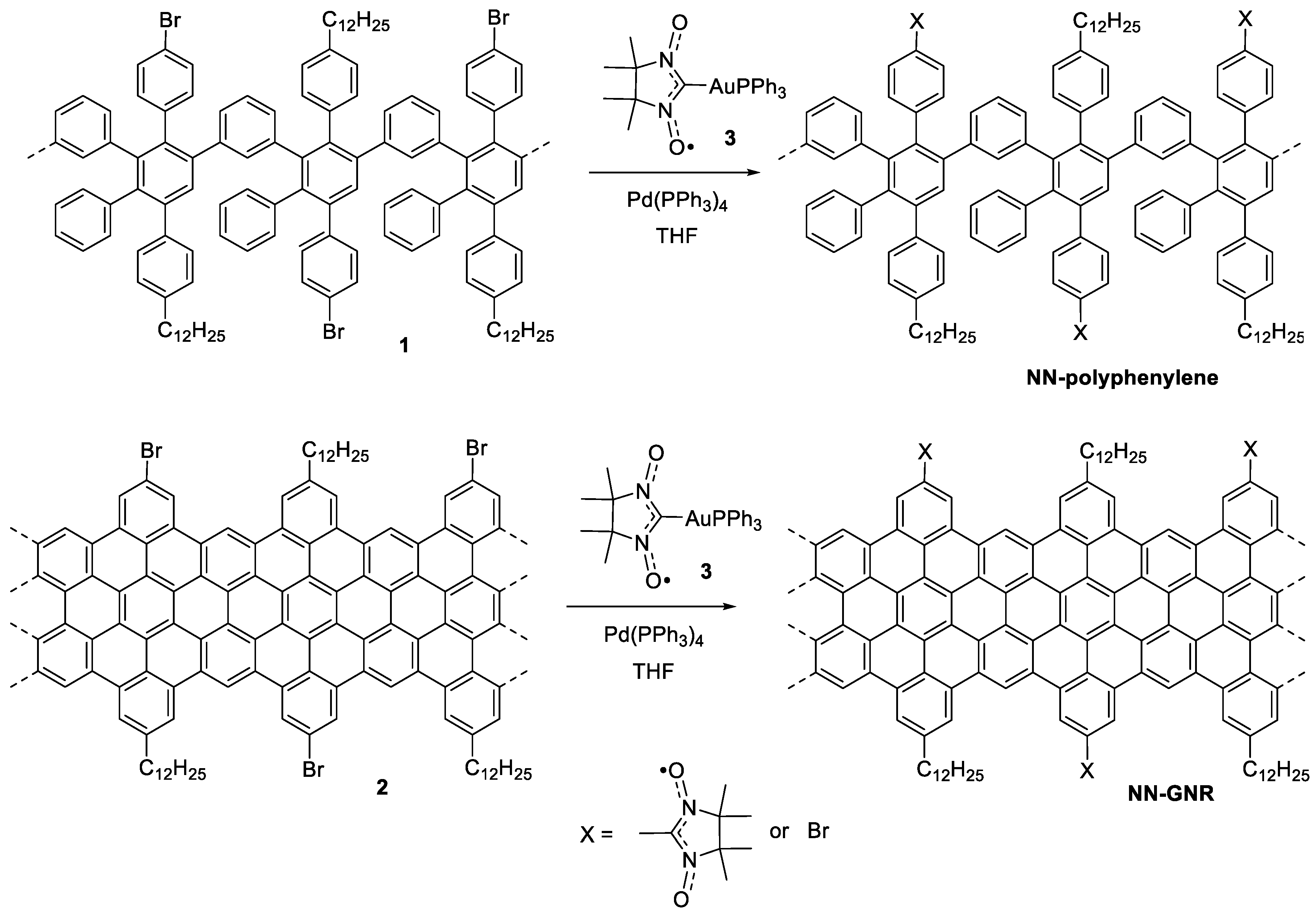
2.1. Compounds Under Study

The studied samples of NN-polyphenylene and NN-GNR were synthesized and characterized previously. These are the same samples that were used in a previous study [8].

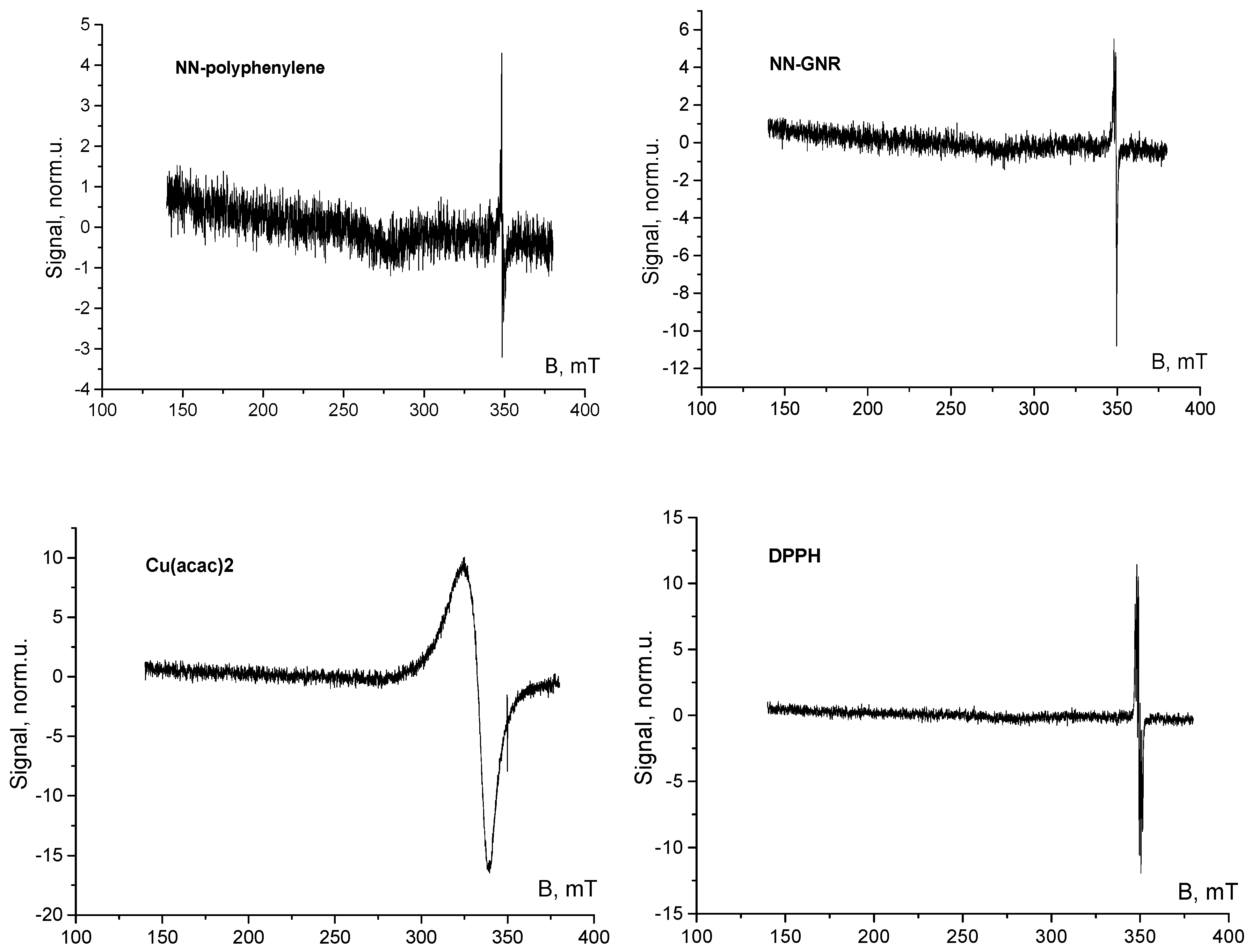
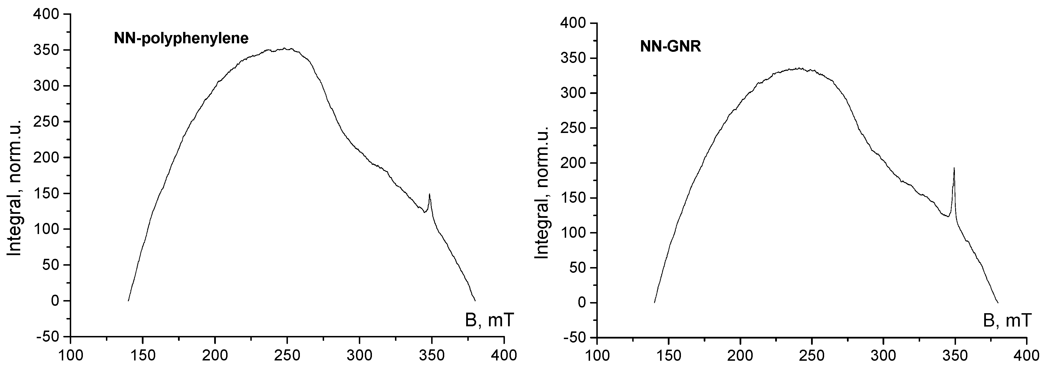
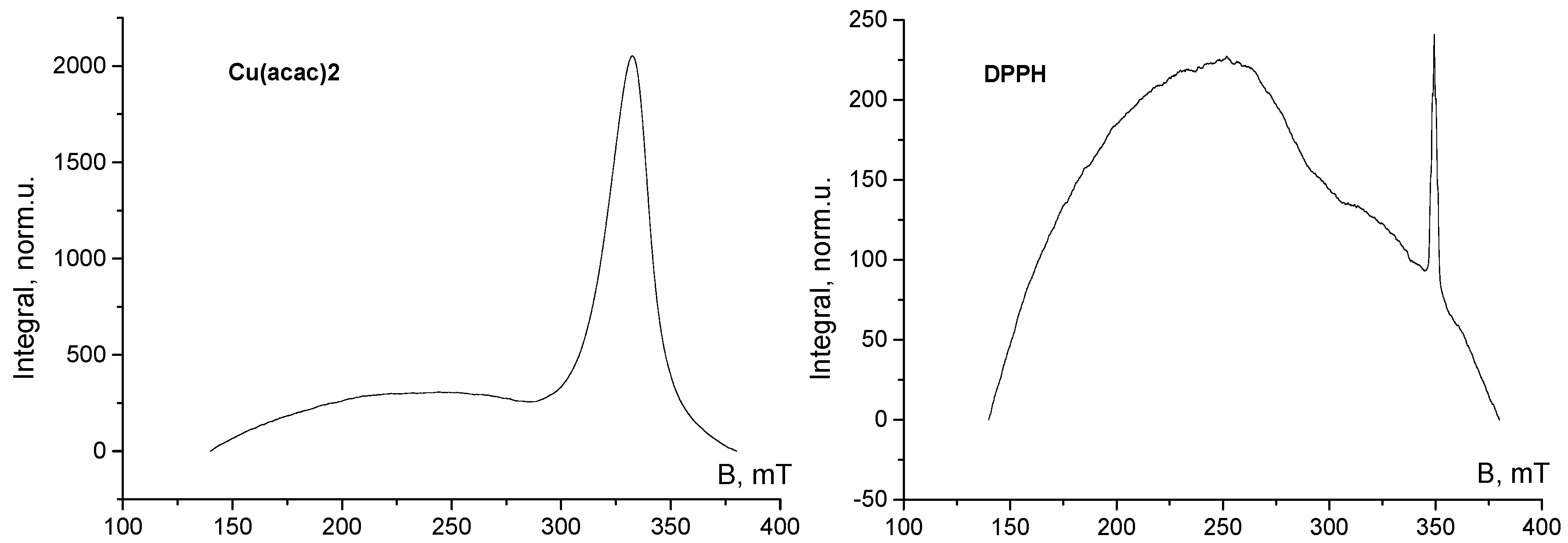
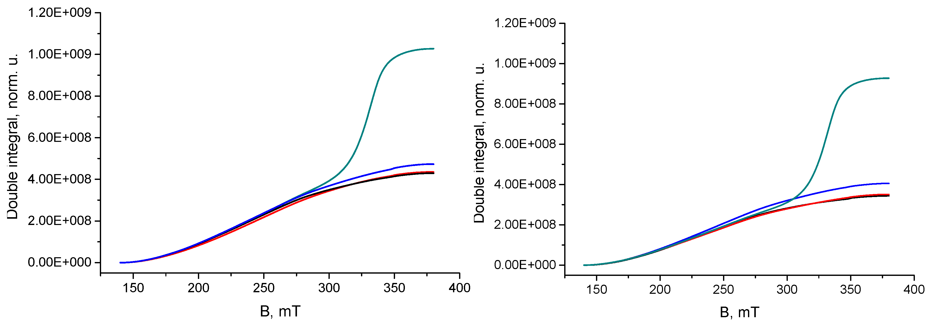
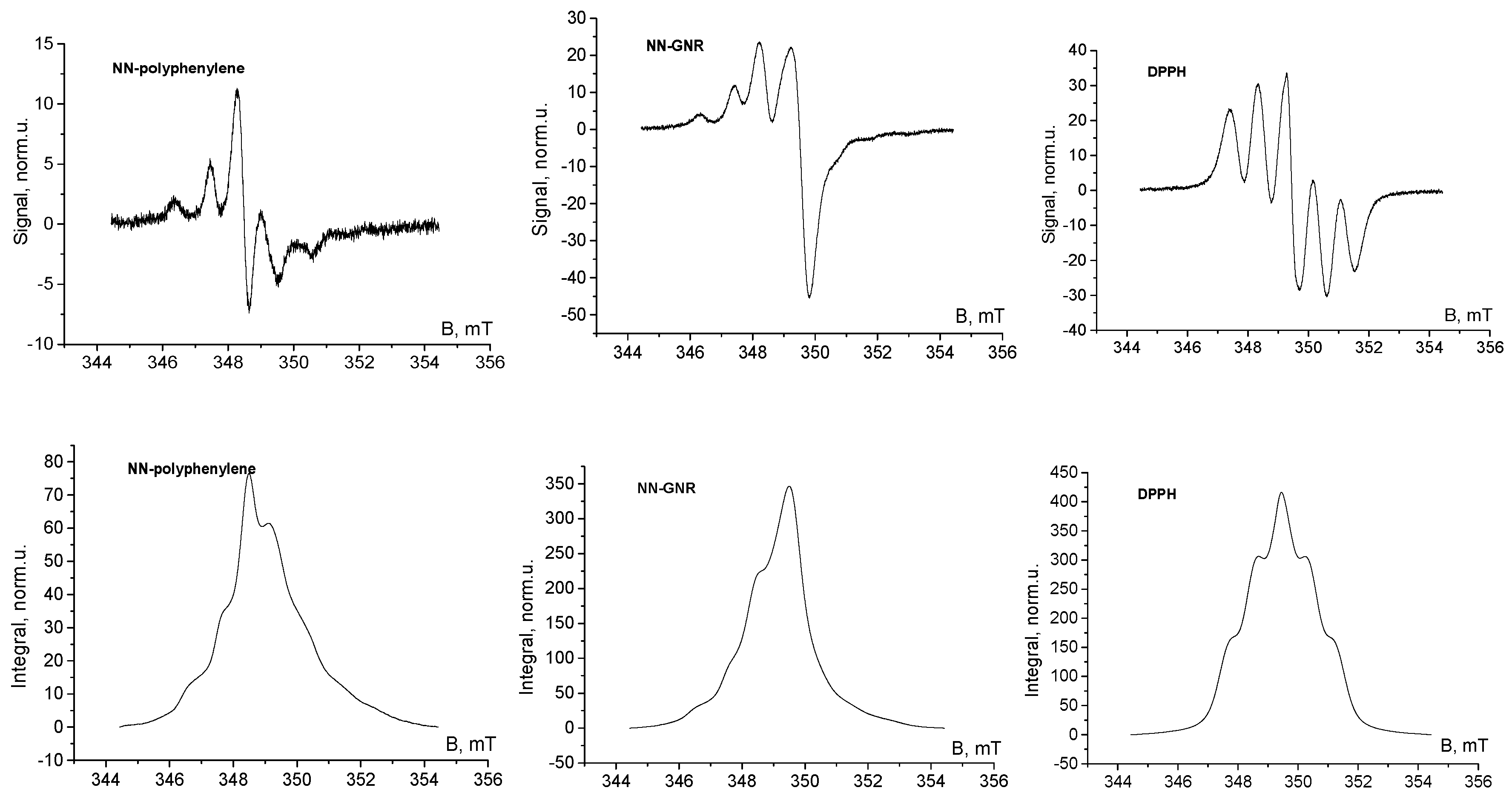
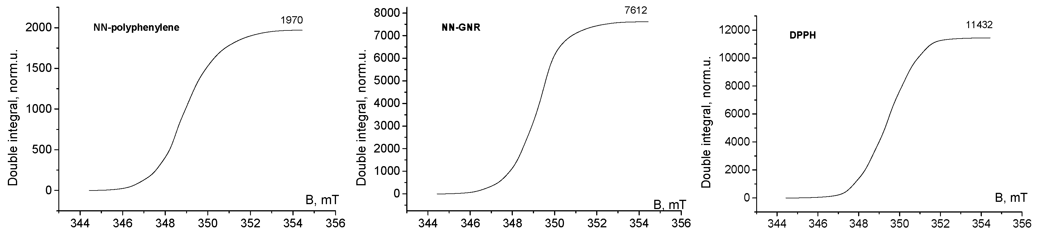
2.2. Sample Preparation, ESR Measurements and Evaluation of Results

All spectra were taken in standard 5 mm outer diameter quartz ESR sample tubes on a Bruker EMX X-band spectrometer with an E4105DR double resonator at room temperature, 2 mW microwave power, and 0.05–0.15 mT modulation at 100 kHz. Four working samples were prepared: 1.00 mg dry NN-polyphenylene (MW* = 628–703), 0.25 mg dry NN-GNR (MW* = 616–692), 0.27 mg dry cupric acetylacetonate (Cu(acac)₂) (MW = 262), 3.0 µg 2,2-diphenyl-1-picrylhydrazyl (DPPH) (MW = 394) in 20 µL toluene. The sample mass was determined by weighing an empty tube on laboratory balances (Ohaus Analytical Plus) to an accuracy of 0.01 mg, putting the sample powder or liquid aliquot inside and weighing the tube again.

As preliminary experiments demonstrated (see below), ESR spectra of both NN-polyphenylene and NN-GNR consisted of a narrow signal in the region g = 2 and a very broad and weak background that on the one hand is practically unavoidable, while on the other hand can hide a broad signal from bulk paramagnetic powder [11]. Therefore, two standard samples for the absolute spin count were prepared. The copper salt, Cu(acac)₂, was used as a standard due to its wide ESR spectrum. It was taken in an amount corresponding to the order of magnitude to the degree of polymer spin labeling (number of spins per molecular unit) of about 100%, to check whether any substantial ESR intensity was hidden in the background. The other reference compound, DPPH, is a standard with a narrow ESR spectrum. It was taken in an amount corresponding to the order of magnitude to the degree of polymer spin labeling of about 1% to check the absolute numbers of spins which generated the intensity contained in the narrow spectrum. Since the required amount of this low-molecular-weight compound was too small for reliable weighing, a solution was prepared and used for sample preparation. While DPPH is stable as a dry powder, DPPH solution in toluene gradually degrades with a characteristic lifetime of about one week, changing color from purple-blue to pale yellow. Fresh solution and sample were prepared as needed. The sample could be considered as a stable standard over the course of measurement taken over the course of several hours.

Additionally, two witnesses having a wide and a narrow ESR spectra of intensities comparable to the four samples were prepared using small crystals of dry Cu(acac)₂ and DPPH, respectively, without noting their exact masses. To avoid additional ambiguities related to different sensitivities of the two sections of the double resonator, the spectra were taken using the witnesses with similar spectral types, Cu(acac)₂ for wide spectra or DPPH for narrow spectra, as follows. One of the witnesses was placed in the reference chamber (front section) of the double resonator, then the four samples were placed into the other chamber. The spectrometer was tuned and pairs of the spectra for the witness and for the sample were recorded. The series was then repeated with the other witness. The measurements were independently repeated over three days, each time preparing a fresh sample of DPPH. All spectra were recorded in identical conditions within the series with wide and narrow witnesses, covering the range of 240 mT for the wide witness and 10 mT for the narrow witness centered at g = 2. The spectra from the samples were normalized by the maximum of the spectrum of the witness for the narrow witness series and by the second integral of the spectrum of the witness for the wide witness series. In the spectra and their integrals, given below, the absolute scales of vertical axes can be directly compared within each group of spectra of the same type.

The described procedure of measuring with standards and against witnesses may seem unnecessarily complicated, but this was done deliberately to handle the problem of the broad background as effectively as possible. The very weak and very broad signals arise due to a combination of factors, including the resonator, sample tubes and eddy currents, and are present as the slowly varying baseline in any real instrument. The resonator is clean, but still has traces of paramagnetic ions from the ambient atmosphere on its walls, as does the waveguide. Sample tubes, although made from suprasil and having calibrated dimensions, still establish slightly different distributions of microwave field in the cavity. Even different repeats (with sample tube removal and installation in the cavity) of the same sample yielded slightly varying backgrounds at the scales reported in this work. To demonstrate what provides information and what is unavoidable natural variation, two characteristic series of (double-integrated) spectra are shown in Figure 3. Furthermore, the background was not identical in the two chambers of the dual resonator, which is the reason for performing the experiments with additional witnesses, in such a manner so as to never compare spectra from different resonators. Instead, a sample with a spectrum similar to that which one would expect was placed in the reference cavity, and then all the analyzed samples—including standards—were placed, in turn, in the working cavity, measured, and normalized to this witness. This completely bypasses the problem of different and unaccountable variations in the backgrounds in two halves of the resonator. Finally, the background was not subtracted before performing integrations of the spectra, because in this case it was more detrimental than helpful. Instruments normally subtract backgrounds automatically, which is very convenient when working with commonly recorded narrow spectra. However, when dealing with very weak and broad spectra—for which a second additional integral will be needed—subtracting a background can be disastrous, as very slight variations in what is subtracted can produce wildly varying results after two integrations. It is much safer to leave everything as recorded and judge the results by eye

The purpose of performing these experiments that have issues with a noisy background was to verify that there is not much useful signal, if any, contained in the broad spectrum, so that the quantitative estimates can then be confined to much less complicated narrow spectra. A broad spectrum could, in principle, have been expected for these systems, as they might have some form of ferromagnetic resonance signals. As described further below, none were found (at least at room temperature), and so the observed narrow spectra could indeed be interpreted as spectra from localized spin labels that bear the useful signal. Therefore, the relative degrees of spin labeling (R) were estimated from the second integrals of the narrow spectra (I), the masses of the samples (m) and molecular weights of the compounds (M) as R₁/R₂ = (I₁M₁m₂)/(I₂M₂m₁). Then, taking the degree R for DPPH as 100%, the degrees R for NN-polyphenylene and NN-GNR were estimated as 0.8% and 1.3%, respectively.

The evaluation described in detail above was performed in our Novosibirsk Lab. The same samples were also independently evaluated in a different laboratory in the UK on a different Bruker EMX system to give a radical substitution of 1.2% for NN-polyphenylene and a radical substitution of 1.3% for NN-GNR (preliminary data from Prof. Lapo Bogani, University of Oxford). This data is based on the double integral and a 3-D EPR image determination by Bruker. This match between two independent evaluations in different laboratories is most encouraging, and lends us a certain degree of confidence in these numbers and the procedure itself. Therefore, it was deemed desirable to be prepared for this publication. This is certainly just an estimate and only provides a ballpark value, so no error evaluation for the given values was attempted. A reader interested in the possibility of the statistically consistent evaluation of quantitative ESR measurements is referred to works by Nicola Yordanov [12,13,14] and to [15]. The next section provides a concise step-by-step exposition of our study.

3. Results and Discussion

Figure 1 shows a representative set of raw spectra from the four samples recorded over the broad range of 240 mT and normalized by the signal from the wide witness (Cu(acac)₂). Figure 2 depicts their first integrals.

All spectra had an unavoidable broad and weak background, against which much narrower spectra were present for NN-polyphenylene, NN-GNR and DPPH, while the spectrum for Cu(acac)₂ showed a broader signal from the Cu²⁺ ion. All spectra showed approximately the same wide background, which was present even for DPPH, which is guaranteed to be free from such a wide intrinsic signal. Therefore, the observed background is an unavoidable experimental artifact when recording such spectra (very wide spectral range for very weak signals). The copper sample also showed the expected broad signal in the range 300–350 mT. If the sample compounds possessed any paramagnetic signal from localized centers with a broad spectrum and in an amount corresponding to almost a 100% degree of spin labeling, a similar broad line would have been expected, but this was not observed.

Although the background looks rather benign in the original modulated CW ESR spectra, determination of the absolute spin counts in the samples requires double integration of the spectra, which completely swamps the narrow spectra from organic radicals, leaving only the omnipresent and overwhelming background. Two typical groups of double-integrated spectra are shown in Figure 3. Results from two independent series are given to illustrate the inevitable variability of such spectra and demonstrate that the broad signals for NN-polyphenylene and NN-GNR—which almost reproduced the signal for DPPH—do not bear any substantial signal from the spins of the samples, which is evident in the spectra for Cu(acac)₂. The second step after 300 mT for the copper standard contributes about the same second integral value as that of the total background. If the polymers were all radicals, their curves would also have reached the top of this step, but this was not observed. The second integral curve for the DPPH standard looks similar to the curves for the sample compounds, while, as mentioned above, its background did not contain any contribution from localized paramagnetic centers in the sample itself. Therefore, the broad shallow background was not attributed to paramagnetic centers in the sample and is a universal artifact. To reiterate, we are talking about very weak and very broad signals that are not related to paramagnetic centers in the sample or standard (DPPH) compounds. This cycle of measurements was repeated several times with freshly prepared DPPH samples and with different ordering of samples in the measurement sequence, yielding approximately the same result: all samples had the same shallow background, and the copper standard had the expected additional paramagnetic signal, which reliably exceeded the level of the background. The conclusion at this stage is that sample compounds NN-polyphenylene and NN-GNR did not contain ESR-active localized paramagnetic centers with broad spectra at the level of spin labeling of 10% or higher.

Figure 4 shows a representative set of spectra for the three “organic” radicals recorded over the range of 10 mT, centered at g = 2, and their respective first and second integrals. The three spectra had comparable widths and intensities (which was the purpose of preparing a 3 µg DPPH standard) and completely fit inside the covered field range. As the integrated spectra clearly show, this range was sufficient to capture the entire resolved spectrum and obtain the corresponding spin counts, without any significant contamination from the omnipresent background. The numbers indicated in the top-right corners of the figures for second integrals are the sought absolute spin counts in arbitrary (but identical) units. These were converted into the degree of spin labeling as described above.

The partially resolved spectra for NN-polyphenylene and NN-GNR generally corresponded to the familiar five-line hyperfine structure from NN (five lines from two nearly equivalent nitrogens) with partially restricted mobility, while the spectrum for DPPH reproduced the known solution spectrum for this stable radical. Although the label in the two samples was the same, it was attached to different backbones. This indicates that the graphene nanoribbon is flatter and more rigid than the polyphenylene backbone, and exerts a different orienting and ordering effect on the attached labels. No spectral simulation was attempted in this work. This would probably be a daunting task, and is beyond the scope of this report. It is not needed for the intended purpose, for which just the second integral suffices. The suggested procedure bypasses this need for spectral simulation, which is one of its positive properties with regard to balancing the problems with background. Finally, we should stress that our analysis, based on measurements at only one temperature, is only valid for non-interacting spins, when the integrated signal intensity only scales with the absolute spin counts and the universal Curie law for the average magnetic moment of the spin in the thermostat in an applied magnetic field. This seems reasonable for the obtained low degrees of spin labeling in NN-polyphenylene and NN-GNR, and for the dilute solution of DPPH used as the standard, but should be kept in mind for the more complex or magnetically-concentrated systems that may be encountered.

4. Conclusions

In this short contribution, we provide a detailed description of a procedure developed to evaluate the degree of spin labeling of a functional material by estimating the absolute numbers of spins in a set of samples with CW ESR and apply it to a polyphenylene-based polymer and its graphitized-derivative-bearing stable nitronyl nitroxide substituents. For these particular systems, the degrees of spin labeling were found to be approximately 0.8% and 1.3%, respectively, which are rather low. Such estimates of the absolute amounts of stable spin labels in otherwise magnetically intricate materials may be useful for developing novel synthetic approaches to prepare modified graphene systems and complement the more advanced ESR studies aimed at functional applications of these novel materials.

References

- Castro Neto, A.H.; Guinea, F.; Peres, N.M.R.; Novoselov, K.S.; Geim, A.K. The electronic properties of graphene. Rev. Mod. Phys. 2009, 81, 109–162. [Google Scholar] [CrossRef]
- Recher, P.; Trauzettel, B. Quantum dots and spin qubits in graphene. Nanotechnology 2010, 21, 302001. [Google Scholar] [CrossRef] [PubMed]
- Meunier, V.; Souza Filho, A.G.; Barros, E.B.; Dresselhaus, M.S. Physical properties of low-dimensional sp2-based carbon nanostructures. Rev. Mod. Phys. 2016, 88, 025005. [Google Scholar] [CrossRef]
- Pesin, D.; MacDonald, A.H. Spintronics and pseudospintronics in graphene and topological insulators. Nat. Mater. 2012, 11, 409–416. [Google Scholar] [CrossRef] [PubMed]
- Trauzettel, B.; Bulaev, D.V.; Loss, D.; Burkard, G. Spin qubits in graphene quantum dots. Nat. Phys. 2007, 3, 192–196. [Google Scholar] [CrossRef]
- Kunstmann, J.; Özdoğan, C.; Quandt, A.; Fehske, H. Stability of edge states and edge magnetism in graphene nanoribbons. Phys. Rev. B 2011, 83, 045414. [Google Scholar] [CrossRef]
- Barone, V.; Hod, O.; Scuseria, G.E. Electronic structure and stability of semiconducting graphene nanoribbons. NANO Lett. 2006, 6, 2748–2754. [Google Scholar] [CrossRef] [PubMed]
- Slota, M.; Keerthi, A.; Myers, W.K.; Tretyakov, E.; Baumgarten, M.; Ardavan, A.; Sadeghi, H.; Lambert, C.J.; Narita, A.; Müllen, K.; et al. Magnetic edge states and coherent manipulation of graphene nanoribbons. Nature 2018, 557, 691–695. [Google Scholar] [CrossRef] [PubMed]
- Narita, A.; Wang, X.-Y.; Feng, X.; Müllen, K. New advances in nanographene chemistry. Chem. Soc. Rev. 2015, 44, 6616–6643. [Google Scholar] [CrossRef] [PubMed]
- Eaton, G.R.; Eaton, S.S.; Barr, D.P.; Weber, R.T. Quantitative EPR; Springer Science & Business Media: New York, NY, USA, 2010; 185p. [Google Scholar]
- Potapov, A.I.; Stass, D.V.; Fursova, E.Y.; Lukzen, N.N.; Romanenko, G.V.; Ovcharenko, V.I.; Molin, Y.N. Searching for the Exchange Shift: A Set of Test Systems. Appl. Magn. Reson. 2008, 35, 43–55. [Google Scholar] [CrossRef]
- Yordanov, N.D. Quantitative EPR spectrometry—“State of the art”. Appl. Magn. Reson. 1994, 6, 241–257. [Google Scholar] [CrossRef]
- Yordanov, N.D.; Ivanova, M. The present state of quantitative EPR spectrometry: The results from an international experiment. Appl. Magn. Reson. 1994, 6, 333–340. [Google Scholar] [CrossRef]
- Yordanov, N.D.; Christova, A. DPPH as a primary standard for quantitative EPR spectrometry. Appl. Magn. Reson. 1994, 6, 341–345. [Google Scholar] [CrossRef]
- Kooser, R.G.; Kirchmann, E.; Matkov, T. Measurements of spin concentration in electron paramagnetic resonance spectroscopy preparation of standard solutions from optical absorption. Concept. Magn. Reson. 1992, 4, 145–152. [Google Scholar] [CrossRef]
© 2019 by the authors. Licensee MDPI, Basel, Switzerland. This article is an open access article distributed under the terms and conditions of the Creative Commons Attribution (CC BY) license (http://creativecommons.org/licenses/by/4.0/).
Share and Cite
Stass, D.; Tretyakov, E. Estimation of Absolute Spin Counts in Nitronyl Nitroxide-Bearing Graphene Nanoribbons. Magnetochemistry 2019, 5, 32. https://doi.org/10.3390/magnetochemistry5020032
Stass D, Tretyakov E. Estimation of Absolute Spin Counts in Nitronyl Nitroxide-Bearing Graphene Nanoribbons. Magnetochemistry. 2019; 5(2):32. https://doi.org/10.3390/magnetochemistry5020032
Chicago/Turabian StyleStass, Dmitri, and Evgeny Tretyakov. 2019. "Estimation of Absolute Spin Counts in Nitronyl Nitroxide-Bearing Graphene Nanoribbons" Magnetochemistry 5, no. 2: 32. https://doi.org/10.3390/magnetochemistry5020032
APA StyleStass, D., & Tretyakov, E. (2019). Estimation of Absolute Spin Counts in Nitronyl Nitroxide-Bearing Graphene Nanoribbons. Magnetochemistry, 5(2), 32. https://doi.org/10.3390/magnetochemistry5020032