Reverse Curve Fitting Approach for Quantitative Deconvolution of Closely Overlapping Triplets in Fourier Transform Nuclear Magnetic Resonance Spectroscopy Using Odd-Order Derivatives

Abstract

A new deconvolution strategy, reverse curve fitting, was developed to determine peak positions and independent intensities of overlapping Fourier transform (FT) nuclear magnetic resonance (NMR) bands. From the third-order derivative of the overlapping band, the peak position was estimated from its zero-crossing point and the peak intensity was quantitated by partial curve matching with its primary maxima. Every matched peak in the overlapping band was dismembered in turn to weaken the overlap until an independent peak was filtered out. The deconvolution can be refined progressively by manually tuning the peak positions and peak widths. In a simulation study, a closely overlapped ¹³C NMR triplet (overlapping degrees between 0.5 and 1.0) at a signal-to-noise ratio (SNR) of 20:1 was quantitatively deconvoluted by our reverse curve fitting procedure with a routine denoising technique. The noise interference and denoising technique were also studied in the simulation. A real FT-NMR overlapping band of Ethylbenzene (300 MHz) was satisfactorily deconvoluted and compatible with higher resolution literature spectral data. A more complicated overlapping NMR band of Tetraphenyl porphyrin was studied as well. This new approach to the deconvolutions is applicable to other FT spectroscopies.

1. Introduction

Fourier transform (FT) nuclear magnetic resonance (NMR) spectroscopy is one of the dominant analytical methods in chemistry [1]. Its line shape is determined by complex interactions between nuclear spins, relaxation times, and a convolution result of the sampled signal with a window function. The blended signals can cause overlapping in the NMR spectrum. The overlapping distorts individual line shape and affects determinations of the line position, peak intensity, and area. Several recent books have summarized many existing technologies and algorithms for resolution enhancements [2,3,4]. New advances empowered us to resolve the overlapping bands more efficiently and more precisely [5,6,7,8,9,10,11]. Even high-performance NMR spectrometers may not resolve overlapping peaks well in biomolecular studies [12]. Spectroscopists can choose or develop a suitable deconvolution method in the light of current experimental situations: How many peaks are there in a band? How closely overlapping are they? And what is the analytical threshold? etc.

According to overlapping degrees stipulated by Vandeginste and De Galan for an overlapping band of a Gaussian peak with a Lorentzian peak [13], the overlapping degree γ between two adjacent FT peaks ω_j and ω_j+1 (ω_j+1 > ω_j) with an identical full width at half height (FWHM) W can be simplified to be [11]

γ = (ω_j+1 − ω_j)/(W/2) = 2(ω_j+1 − ω_j)/W

(1)

The original formulation of the overlapping degree introduced by Vandeginste and De Galan was complicated because different peak shapes were used in the curve fitting. Since the acquired time domain signals are converted to a frequency spectrum by FT, we should utilize real NMR peak shapes produced by FT from the outset. Based on the study results of Vandeginste and De Galan, Madamms anticipated that the deconvolution of curve fitting could reach its reliable limitation when two peaks separated below an overlapping degree of 0.8 even without the presence of noise [14]. The feasibility of the deconvolution methods strongly depends on the overlapping degrees. Therefore, we graded the overlapping bands into four groups as their overlapping degrees:

(I)

Loose overlap as overlapping degrees γ ≥ 2.0;

(II)

Moderate overlap as γ from 1.0 to 2.0;

(III)

Close overlap as γ from 0.5 to 1.0;

(IV)

Tight overlap as 0 < γ < 0.5.

If the two overlapped peaks of Group I have the same intensity, their overlapping portion will be ≤ 50% respective to each peak. Individual peak vertices of Group I usually are visible when adjacent peaks have no overwhelmingly different intensities with sufficient signal-to-noise ratios (SNRs). The overlapping peaks of Group II crowd into a cluster and some peaks may be fused into the others. They are easily distinguishable by derivative algorithms. The overlapping peaks of Group III are jammed together, and some peaks are not easily perceivable by high-order derivatives. For the tight overlapping bands in the last group, it is difficult to discriminate one peak from another by the derivatives of the peaks. Group IV is the most difficult section to resolve as the peaks often merge into an organic whole without distinguishable boundaries.

Theoretically, conventional FT spectrum peaks display symmetric profiles from harmonic time signals and exhibit the same FWHM if they experience the same free induction decay process [15] (pp. 14–16). The decay is characterized exponentially by the transverse (or so-called spin–spin) relaxation time T₂, and the NMR peak width is inversely proportional to relaxation time. Subtractions are a common practice in NMR spectroscopy to simplify and optimize identification and quantitation works. The intensity of an NMR signal was altered using the difference technique of the nuclear Overhauser effect [1] (pp. 111–112). Thanks to these features, we proposed a novel reverse curve fitting procedure to deconvolute the overlapping bands. This new procedure employs odd-order derivatives to fit one of the edge peaks in an overlapping band, and then the fitted peak is dismembered from the band by individual FT (deconvolution). The peaks in the band are individually removed out until their independent line shapes have been precisely fitted and isolated out. Such a dismembering strategy reverses routine curve fitting process. In this work, we simulated a closely overlapping ¹³C NMR triplet to demonstrate how to implement the reverse curve fitting approach. Then, it was applied to deconvolute a real FT-NMR overlapping triplet, and a real Fourier transform infrared (FT-IR) overlapping triplet.

A general procedure of reverse curve fitting is outlined in

Table 1. A general protocol of reverse curve fitting procedure for deconvolution.

1. Segregate an overlapping band and include a well-separated peak nearby (as a reference) if possible. 2. Set an analytical threshold according to noise level (expected SNR). 3. Perform denoising and/or smoothing with a proper denoising technology, such as Kauppinen’s band-pass filtering and smoothing in time domain signals [15] (p. 172). 4. Isolate the reference peak or predominated peak and estimate its peak width by Hilbert transform. Its position and intensity are deduced from the zero-crossing point and primary maximum of 3rd-order derivative in the frequency spectrum by a partial curve matching (PCM) strategy to imitate a harmonic signal in the time domain. Refine the peak position and intensity to reach the appropriate match with the derivative primary maximum of the reference peak via FT of the imitated time signal. 5. Implement the reverse curve fitting procedure by partially curve matching the primary maxima of the edge peaks and progressively reduce the members in the overlapping band to filter out independent peaks individually. 6. Repeat Step 5 until the intensity and peak width of each filtered-out peak are convergent.

. The readers can refer to the Section 3 for further details.

2. Materials and Methods

2.1. Materials and Curve Fitting Strategy

A 100 MHz Carbon-13 NMR signal was simulated and transformed by edited Python software (version 3.10.14) with noise testing. Proton NMR 300 MHz time domain signals of Ethylbenzene were taken from the commercial software of Acorn NMR Inc. (Livermore, CA, USA) [16]. 5,10,15,20-Tetraphenyl porphyrin (Sigma-Aldrich HPLC grade, >99.0%, Burlington, MA, USA) was dissolved in Chloroform-d (CDCl₃, 99.8%–D, Nanjing Chemical Reagent, Nanjing, China) and analyzed on a Bruker Avance III 400 MHz NMR spectrometer (Billerica, MA, USA). The FT-IR spectrum of 1,1-Dichloroethene was downloaded from the NIST open FT-IR spectral source Quantitative Infrared Database [17]. Third-order derivatives and curve fitting algorithms were used to match their primary maxima until convergent least-square results were achieved.

All of the overlapping spectra studied in this work were well apodized by applying a 3-term Blackman–Harris window function in time domain t relative to their signal acquirement time T:

0.42323 + 0.49755 cos(πt/T) + 0.07922 cos(2πt/T).

2.2. Peak Position and Derivatives

A spectral measurement and the associated curve fitting process always involve determinations of the peak positions. Practical spectral profiles cannot be perfectly reflected by discrete data because the critical parameters of peaks may not coincide with those discrete points, such as peak positions. One of our solutions was to raise the sampling rate of FT spectroscopy by more than 20 times the Nyquist frequency [18] (p. 75). Even-order derivatives have similar problems capturing peak positions. To avoid very high sampling rates and thus to save time, Huguenin and Jones innovated using a zero-crossing point of 5th-order derivatives to trace positions of overlapping peaks [19].

According to derivative formula of a discrete spectrum with a sampling interval ∆ω [11], the third-order derivative D⁽³⁾ is

$${\mathrm{D}}_{\omega +\mathsf{\Delta }\omega /2}^{\left(3\right)}={\displaystyle \frac{A_{\omega +2∆\omega }-3A_{\omega +∆\omega }+3A_{\omega }-A_{\omega -∆\omega }}{{(∆\omega )}^3}};$$

(2)

and the fifth-order derivative D⁽⁵⁾ is

$${\mathrm{D}}_{\omega +\mathsf{\Delta }\omega /2}^{\left(5\right)}={\displaystyle \frac{A_{\omega +3∆\omega }-5A_{\omega +2∆\omega }+10A_{\omega +∆\omega }-10A_{\omega }+5A_{\omega -∆\omega }-A_{\omega -2∆\omega }}{{(∆\omega )}^5}},$$

(3)

where A is the intensity at each sampling point around the individual center frequency ω; and the discrete odd-order derivative is calculated at point ω+∆ω/2. The sampling interval ∆ω should be very small when the sampling rate is sufficient. We rationally assume that the odd nth-order derivative D⁽ⁿ⁾ around the zero-crossing point ω₀ is approximately linear. The closest front and back sampling points of ω₀ are ω_0a and ω_0b, where ω_0b – ω_0a = ∆ω for ω_0a < ω₀ < ω_0b. The simultaneous linear equations of derivative D⁽ⁿ⁾ are

$$\left\{\begin{array}{c}{D}_{{\omega }_{0a}+\mathsf{\Delta }\omega /2}^{\left(n\right)}{=D}^{\left(n\right)}{(\omega }_{0a}) \cong { K \omega }_{0a}+B\\ D_{{\omega }_{0b}+\mathsf{\Delta }\omega /2}^{\left(n\right)}{=D}^{\left(n\right)}{(\omega }_{0b}) \cong { K \omega }_{0b}+B\end{array}\right.,$$

(4)

where K is the slope and B is the intercept depending on the nth order of the derivative. They are easily solved to be

K = [D⁽ⁿ⁾(ω_0b) − D⁽ⁿ⁾(ω_0a)]/∆ω;

(5a)

B = D⁽ⁿ⁾(ω_0b) − [D⁽ⁿ⁾(ω_0b) − D⁽ⁿ⁾(ω_0a)]ω_0b/∆ω,

(5b)

or = D⁽ⁿ⁾(ω_0a) − [D⁽ⁿ⁾(ω_0b) − D⁽ⁿ⁾(ω_0a)]ω_0a/∆ω. Since derivative D⁽ⁿ⁾ = 0 at its zero-crossing point,

ω₀ ≅ −B/K.

(6)

For the discrete odd-order derivatives, recall adding the term ∆ω/2 above ω₀ because that term must be included.

The zero-crossing point of derivative D⁽³⁾ will be used to locate the peak position. A single ¹H (proton) NMR peak was imitated and is shown in Figure 1 (blue spectrum), and the peak center at 7.0 ppm coincides with the zero-cross points of its 3rd-order and 5th-order derivatives, D⁽³⁾ (brown line) and D⁽⁵⁾ (pink line).

3. Results

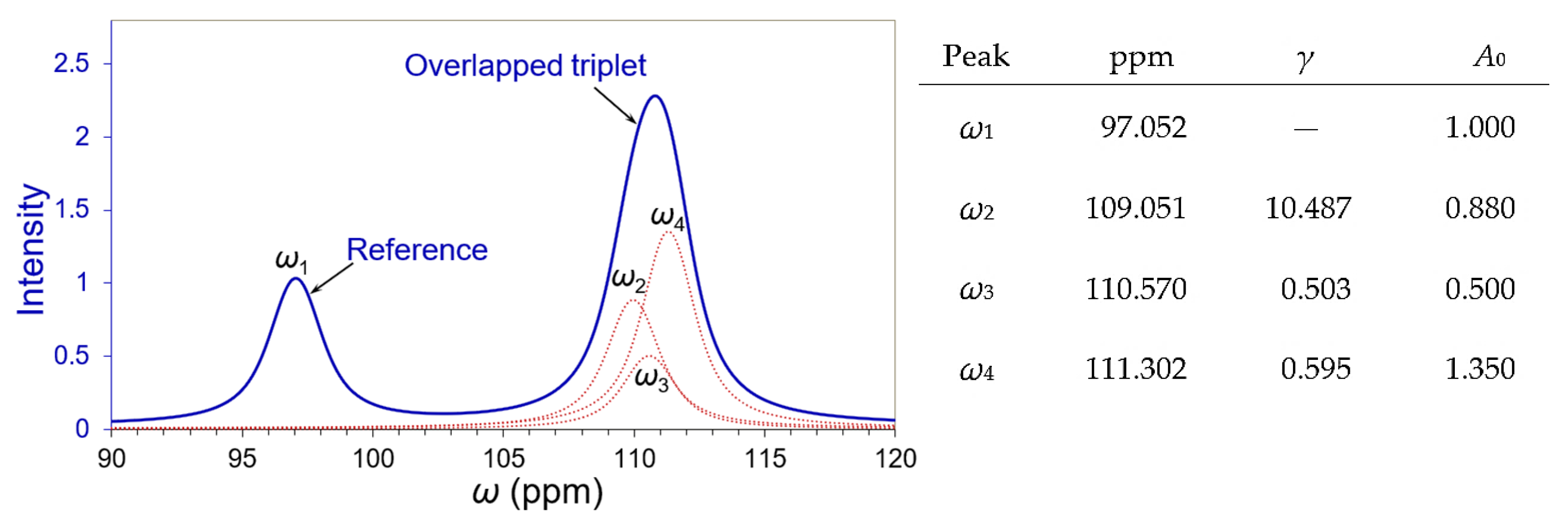
3.1. Deconvolution of a Simulated Overlapping Triplet

Solid-state Carbon-13 nuclear magnetic resonance (NMR) spectroscopy provides a powerful probe to study structural biology. A closely overlapped triplet with a well-separated reference peak of the 100 MHz ¹³C NMR spectrum was simulated and is presented in Figure 2, likened to experiments for amyloid architecture [20]. Its signal decay coefficient was devised to be 628.319 (2π × 100 Hz) for a FWHM of about 1 ppm at a sampling rate 8 times the Nyquist frequency for a range of 50 to 180 ppm (1024 data points in total). The principal simulation parameters (peak position in ppm, overlapping degree γ, and peak intensity A₀) were specified beside the spectrum, as shown in Figure 2. For more simulation details, please refer to Section S1 and Figure S1 in the Supporting Information.

It is important to have a reference peak in deconvolution: (a) for the evaluation of the peak width and the decay coefficient of its time signal; (b) as a ruler for peak intensities; and (c) for minimal consideration to peak shape in the deconvolution, regardless of whether it is Gaussian, Lorentzian, Voigt, or Tsallis [21]. The three peaks in the triplet were merged wholly as their overlapping degrees ≈ 0.5 to 0.6. All peak vertices were not caught by the sampling data intentionally. After being apodized by a 3-term Blackman–Harris window, the FWHM of an individual independent peak W ≈ 2.46 ppm was estimated from the reference peak ω₁ in Figure 2. Their overlapping degrees were calculated against a semi-FWHM ≈ 1.23 ppm.

The most common noise that appeared in FT spectroscopy was white noises. It is necessary to denoise well in advance of spectral deconvolution. We added white Gaussian noise into the spectrum of Figure 2 at an SNR = 20:1 (versus the smallest peak ω₃) for the noise tests (refer to Section S2 and Figure S2 in the Supporting Information). As shown in Figure 3a, the amplified noise dominates derivative D⁽³⁾, and Kauppinen’s band-pass filtering technology had demonstrated good success for the denoising of FT spectroscopy [11]. The entire spectrum of Figure 3a was denoised by inverse FT denoising technology using Kauppinen’s band-pass filter (a boxcar window was applied to segregate the time domain raw signal) [15] (p. 172). The effectiveness of the denoising on the spectral peaks is better than at their baseline as the primary maxima of the recovered D⁽³⁾ matched well with the authentic ones. This assured us to begin with the isolation of reference peak ω₁ by cutting off the triplet along the red dashed line in Figure 3b. The decay profile in the time domain of the isolated peak was measured via Hilbert transform [22] and analyzed by a linear regression as shown in Figure 4. Its decay coefficient = 627.265 (s⁻¹), with R-square = 0.989, deviated merely 0.168% from its theoretical value of 628.319 (s⁻¹), which ensured the FWHMs of the overlapping peaks to be accurately determined. When an isolated peak is transferred into the time domain by Hilbert transform, we scan plot its ln|magnitude| versus time t, as displayed in Figure 4. If the peak is pure, its linear regression should be near a straight line. Otherwise, the line would appear bent away from linearity.

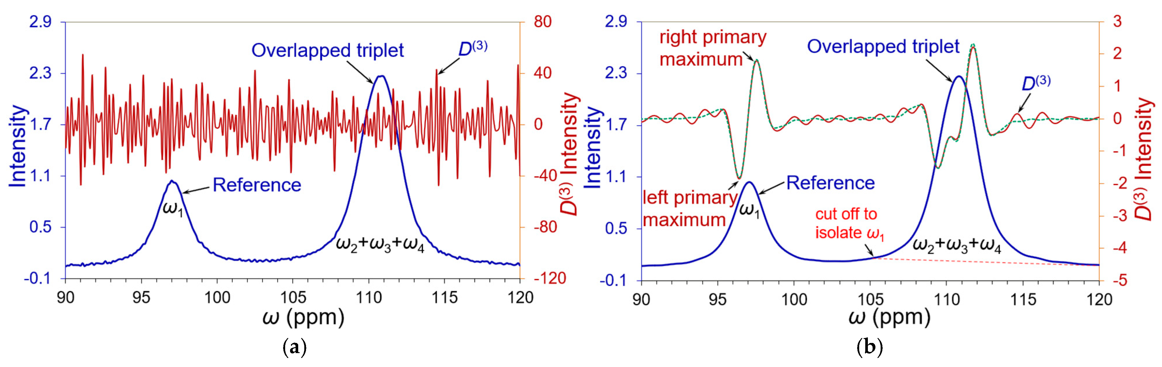
3.2. Partial Curve Matching Strategy and Reverse Curve Fitting Procedure

Although reference peak ω₁ was well separated in Figure 3b, its apparent intensity was inflated slightly (about 4.4%) from a distant overlapping of the triplet. As its D⁽³⁾ left primary maximum suffers less overlapping interference than its right one from the triplet, we introduced a partial curve matching (PCM) strategy to deduce its independent peak intensity from the left primary maximum. The apparent intensity and the D⁽³⁾ zero-crossing point of peak ω₁ were taken as its initial peak intensity and position. An independent ω₁ was imitated, as shown in Figure 5a, by FT using the assessed decay coefficient and the same apodizaion window in time domain. The left primary maximum was partially matched for its 10 discrete spectral data as those red spots in Figure 5a. Their matching errors were minimized by manually tuning the peak position and intensity through a simple least-square analysis [23]. We obtained ω₁ ≈ 97.056 ppm and A₀ ≈ 1.013 (very close to its simulation values in Figure 2). The 10 data points should be located within a less overlapping portion. More data points can be added if they do not affect the accuracy of the deconvolution and when time consumption is not critical.

Any overlapping band must have two edge peaks as the band boundary: front and back edge peaks. The edge peak usually demonstrates noticeable derivative primary maxima if its neighbor does not have overwhelming intensity. We started matching back edge peak ω₄ of the triplet in Figure 5b because of its outstanding right primary maximum. The initial position and intensity of peak ω₄ were estimated from its D⁽³⁾ zero-crossing point and apparent intensity A₀₄ (or reckoned against the peak height of the reference peak ω₁) to produce a harmonic time signal 2A₀₄cos(ω₄t). This initial time signal was converted to a single NMR peak by FT and implemented D⁽³⁾ derivative. The right primary maximum of edge peak ω₄ should be matched appropriately by manually tuning the zero-crossing point and intensity of the initial signal several times (note that a perfect fit is not expected at this stage as it is not yet an isolated peak). The matched ω₄ was then subtracted from the triplet to make the front edge of peak ω₂ emerge promptly, as shown in Figure 5c. Such a removal of the matched peak(s) from the overlapping band is called “dismembering”.

We applied the same process to estimate peak ω₂ in Figure 5c from its left primary maximum of D⁽³⁾. Because edge peak ω₄ was never evaluated by dismembering any other overlapping peak, it was rematched in Figure 5c after the matched ω₂ was removed. This dismembering cycle was counted as Cycle-0 because only two edge peaks were able to be taken away. The middle peak ω₃ appeared as a single peak in Figure 5d after dismembering the two matched edge peaks, ω₂ and ω₄. Then, the middle D⁽³⁾ curve of the filtered ω₃ in Figure 5d was chosen as its matching portion to obtain its initial peak intensity A₀₃, position ω₃, and harmonic time signal 2A₀₃cos(ω₃t). We found that the PCM on the middle D⁽³⁾ portion can minimize the uncertainties of its primary maxima and the matching error of peak ω₃. Now we can repeat the above PCM process to filter out the individual independent peak from the triplet in turn by dismembering the other two peaks. This is a completion cycle specified as Cycle-1. The curve fitting regressions use a group of symmetric profiles to fit all spectral data with the least errors. The PCM/dismembering operations exactly reverse the curve fitting procedure to filter out each independent peak. Therefore, we call our new method reverse curve fitting. More cycles of the reverse curve fitting procedure can be continued until reliable results are achieved. A general convergence criterion of reverse curve fitting was set to be ≤2.0% in the peak intensities and peak positions of every deconvoluted peak between 2 consecutive dismembering cycles.

All of the study data in this work are reported with three decimals for the sake of precision. The deconvolution process of the triplet is sketched in Figure 6. The deviation (%) of front edge peak ω₂ is depicted by a blue line; back edge peak ω₄ in green; and middle peak ω₃ in brown. The deconvolution achieved quantitative errors below 4.0% (double the convergence criterion ≤ 2.0%) at Cycle-4. Despite the minor denoising distortions in Figure 3b, their influences were expected to cause about a 10% error in the deconvolution for peak intensities of the close overlapping peaks. Residual error analysis helps further examine the convergency of the devolutions. We presented a segmental analysis for the relative residue of the deconvolution at each matched peak position in every dismembering cycle against the native spectrum. The segmental relative residue% of a peak at ω is

(Relative Residue %)_ω = 100(A_i − A₀)/A_ω.

(7)

where A_i is a spectrum composed of all the deconvoluted peaks in a dismembering cycle; A₀ = native spectrum; and A_ω = deconvoluted peak at peak position ω. For example, the deconvolution of edge peak ω₄ achieved its best result (residue% = 0.175%) in Cycle-3 rather than in Cycle-4 (residue% = 0.848%), as shown in Figure 7.

When the spectral quality was improved to an SNR = 40:1 for the same triplet, we repeated the previous process and raised the deconvolution accuracy to <2.0% of the intensity errors with less cycles (at Cycle-3). The deconvolution results regarding these two SNR levels were specified in

Table 2. Deconvolution results of the simulated spectrum of Figure 1 at two different SNR levels.

SNR	Peak	ω2		ω3		ω4
		ppm	A0	ppm	A0	ppm	A0
	Real value	109.951	0.880	110.570	0.500	111.302	1.350
20:1	Deconvoluted (deviation)	109.949 (−0.002%)	0.882 (+0.227%)	110.573 (+0.003%)	0.481 (−3.800%)	111.297 (−0.004%)	1.355 (+0.370%)
	Filtered *	109.950	0.886	110.547	0.480	111.308	1.353
40:1	Deconvoluted (deviation)	109.954 (+0.003%)	0.886 (+0.682%)	110.605 (+0.032%)	0.498 (−0.400%)	111.315 (+0.012%)	1.342 (−0.593%)
	Filtered *	109.949	0.899	110.591	0.500	111.314	1.343

* The filtered peaks provide supplemental verifications to the deconvolution results.

. Our previous deconvolution procedure was solely based on the primary maxima ratio of odd-order derivatives [11]. Now we rely on some dozen data points on the D⁽³⁾ primary maximum portion (PCM strategy) to enhance the deconvolution accuracy.

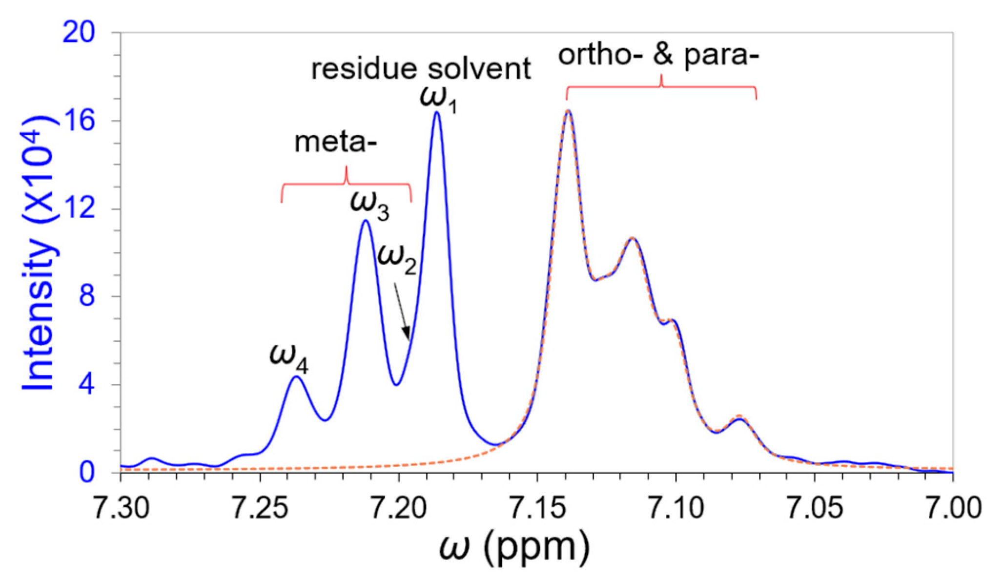
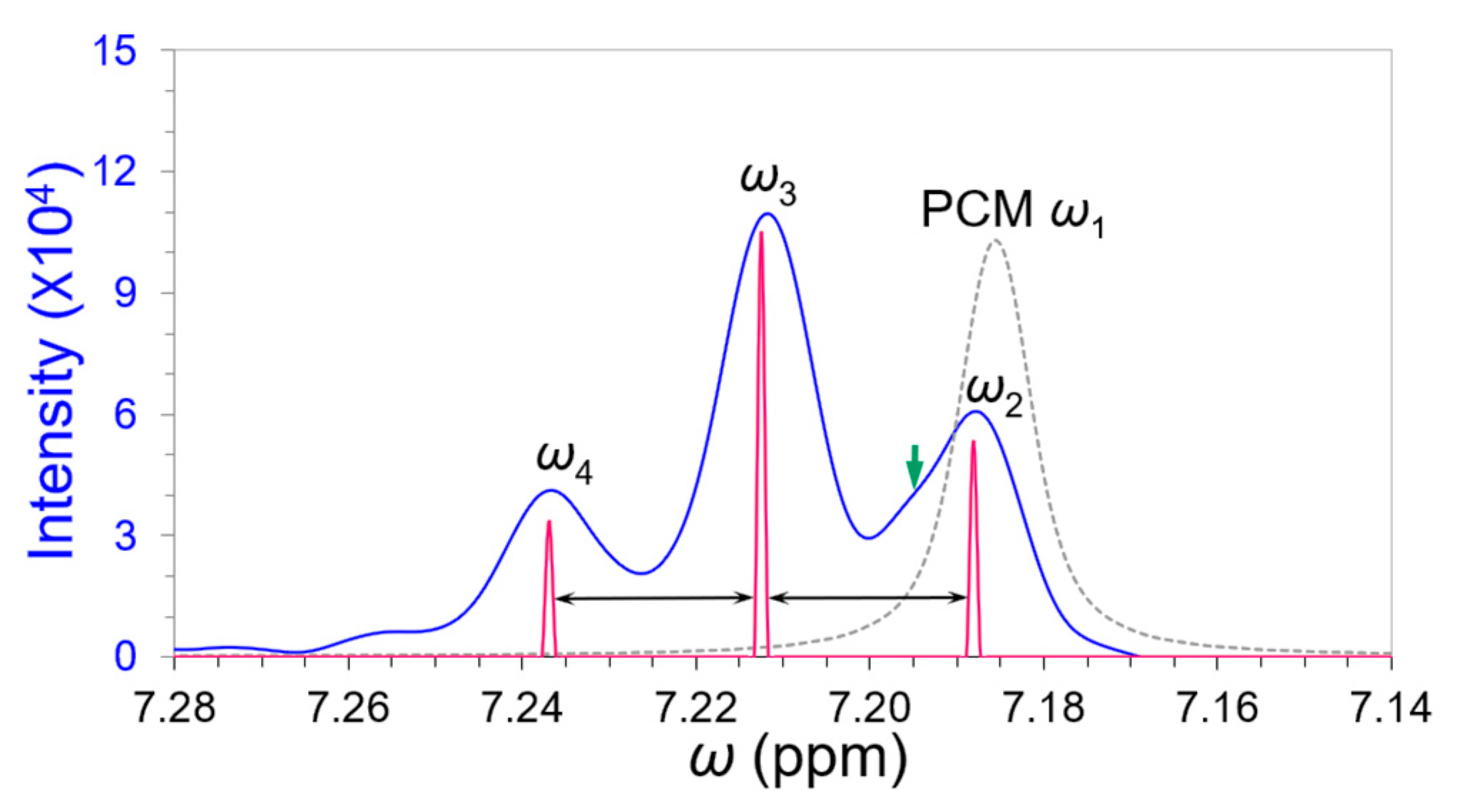
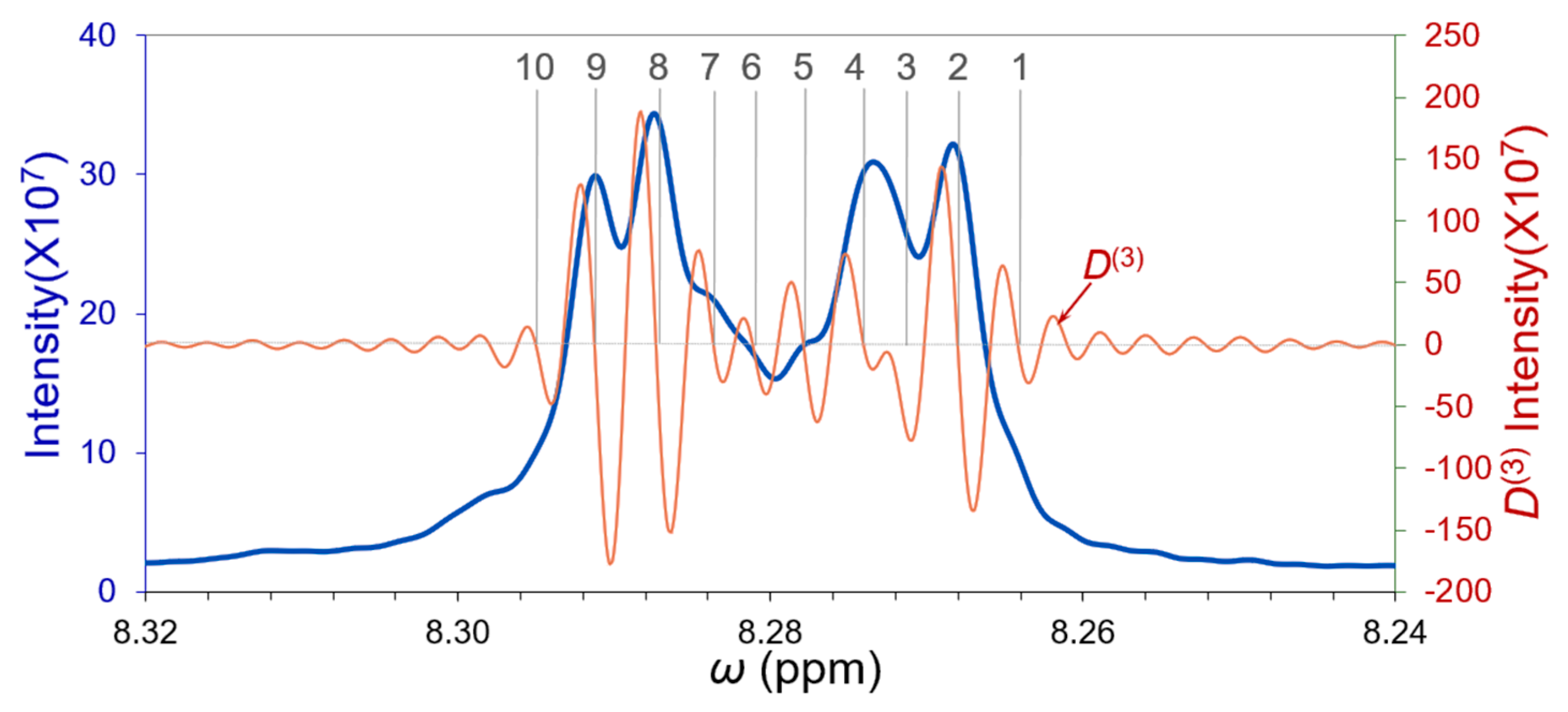
3.3. Deconvolution of the “Closely” Overlapped NMR Peaks

NMR spectroscopy is a powerful technique to study the structures and dynamics of molecules. Deconvolutions of the practical overlapping bands can be more complicated than the above simulation scenarios. We qualitatively deconvoluted a 300 MHz proton NMR magnitude-mode spectrum of Ethylbenzene in our previous work [11]. Because the magnitude-mode overlapping peak intensities are non-additive, the aryl protons were simply deconvoluted by superimpose FT and evaluated by primary maxima ratios of the odd-order derivatives D⁽³⁾ and D⁽⁵⁾ [11]. In this article, we extended our deconvolution study to aryl proton spin–spin coupling, using our reverse curve fitting technology. To avoid the non-additive issue, we specifically studied the absorption-mode spectrum of Ethylbenzene that exhibited two merged bands in 300 MHz NMR as shown in Figure 7. The main acquisition parameters from a QE 300 NMR spectrometer (GE limited of USA, Cincinnati, OH 45215, USA) with a 7 Tesla magnet are [16] a 250 μs dwell time, 4000 Hz scanning bandwidth, 1850 Hz offset frequency, and 0.512 s sampling time, with 2048 data points. The acquired raw signal was reprocessed by interpolating 8 points equivalent to 8 zero-fillings and a 3-term Blackman–Harris apodization window.

We pursued the deconvolution of this NMR band for two reasons: (i) to deal with different peak widths; and (ii) when a peak fuses into a big peak (overlapping degree γ ≤ 0.5). The solvent peak ω₁ (Chloroform-d) is obviously narrower than the other aryl peaks corresponding to meta-, ortho- and para-protons. Meta-proton peak ω₂ fused tightly into solvent peak ω₁ and downfield proton peaks (ω₁ to ω₄), with a similar ortho- and para-proton band imitated and removed along the dashed brown line indicated in Figure 8 to cure their overlapping effects. Fortunately, the intensity of the solvent peak ω₁ was larger than the other peaks in the spectrum, and meta-proton peaks ω₃ and ω₄ were separated moderately. Their decay coefficients can be estimated roughly by isolating each of them approximately, as was performed in the above simulation study. Although the initial decay coefficients could be very imprecise (for example, 8.383 for solvent ω₁ and 11.594 for the largest meta-proton ω₃), they will be refined gradually through the reverse curve fitting process (PCM/dismembering process) to their D⁽³⁾ primary maxima. Different peaks have different peak widths. Because the peak shape and its derivative profile both are evaluated in PCM/reverse curve fitting, they can help find the right peak width of the overlapping band. The deconvolution of the spectrum in Figure 9 (after removing ortho- and para-protons) involved at least two kinds of peak widths, the solvent peak and meta-proton peaks. Their final deconvolution results are summarized in

Table 3. The deconvolution results of Figure 8.

	Peak	ω1	ω2	Unknown	ω3	ω4
	Overlapping γ	–	0.383		3.577	3.512
Cycle-6	ppm	7.186	7.188		7.213	7.237
	A0	103098	53298		104942	33428
	FWHM	0.01004	0.01359		0.01406	0.01359
Filtered *	ppm	7.186	7.187	7.195	7.213	7.237
	A0	101440	53375	1958	104436	33291

* The filtered results are for information only.

.

We must carefully choose the derivative D⁽³⁾ portion in a deconvolution to evade the low-frequency distortions in the NMR spectrum. A common practice is that any evaluated intensity from the D⁽³⁾ primary maxima ratios generally should not be larger than its apparent intensity. The apparent intensity was usually adopted as the initial value of the PCM. We recalled that the overlapping degree in Equation (1) was defined by an identical FWHM. When two overlapping peaks have different peak widths, their overlapping degree should be measured with their reduced peak width. If FWHM of ω₁ is W₁ and FWHM of its overlapping peak ω₂ is W₂, their reduced FWHM W_red is [13]

W_red = 2W₁W₂/(W₁ + W₂).

(8)

The meta-proton triplet was well restored in Figure 10 after dismembering the matched ω₁ whose peak width (0.01004 ppm) was just 70% of that of meta-proton peak ω₃ (=0.01406 ppm). The deconvoluted triplet displayed almost equal spacings and leaning effect in their intensities related to their second-order J-coupling. We detected a tiny peak appearing between peaks ω₂ and ω₃ as indicated by a green arrow at 7.195 ppm in Figure 10. Our analytical threshold was <4.0% by doubling the convergence criterion ≤ 2.0% between the consecutive deconvolution difference in Section 3.1. This tiny unknown peak was not worthy to deconvolute further because its filtered intensity was below our analytical threshold (<4.0% of ω₂ intensity in Table 3). Nevertheless, ω₁, ω₂, and this tiny peak composed of a closely overlapped triplet as their average overlapping degree would be <0.8. The peaks ω₃ and ω₄ played reference roles in this overlapping band, very useful for the evaluation of peak widths and intensities. Our deconvoluted results agreed with the high-resolution NMR spectra of Ethylbenzene at 600 MHz and 920 MHz [24,25], but not so “leaning” as their meta-proton triplets.

A more complicated overlapping NMR spectrum of Tetraphenyl porphyrin was obtained from a Bruker Avance III 400 MHz NMR spectrometer. The main acquisition parameters were a dwell time of 139 μs, scanning bandwidth of 7200 Hz, an offset frequency of 3600 Hz, and a sampling time of 2.272 s, with 16k data points. The acquired raw signal was reprocessed by interpolating 3 points and a 3-term Blackman–Harris apodization window.

An overlapping band of the ortho-phenyl proton NMR spectrum (blue spectrum) was segregated in Figure 11. The zero-crossing points of the 3rd-order derivative (brown spectrum) clearly indicate 10 overlapping peaks by the gray lines. These 10 peaks do not belong to the closely overlapping group graded by us in the Introduction Section. This is interesting to us in deconvolutions with the reverse curve fitting approach. Several peaks among them never matched their filtered independent peaks with their D⁽³⁾ derivative primary maxima, which revealed a broad background underneath these peaks and constituted a closely overlapping band.

For facility in the deconvolution, the peak width of these overlapping peaks was treated rationally to be the same. Their FWHM was evaluated to be 0.003590 ppm from the free induction decay coefficient of the time domain signal and the predominant peak #2 in Figure 11. Since there were no perceptible edge peaks in the band, their deconvolutions started with the three predominant peaks #2, #8, and #9. The initial reverse curve fitting cycle was Cycle-1. We performed 5 cycles of the reverse curve fitting process and the final deconvolution results are displayed in Figure 12 and

Table 4. Deconvolution results of the overlapping band of Tetraphenyl porphyrin in Figure 12.

Cycles	Peaks	1	2	3	4	5	6	7	8	9	10
Cycle-1	ppm A0 (×107)	8.2648 6.094	8.2682 27.565	8.2718 9.845	8.2741 17.376	8.2777 6.558	8.2816 5.334	8.2842 9.997	8.2876 31.055	8.2914 27.207	8.2945 5.194
Cycle-2	ppm A0 (×107)	8.2648 5.975	8.2682 27.920	8.2718 14.314	8.2742 17.580	8.2778 6.713	8.2816 5.891	8.2842 11.694	8.2875 28.813	8.2913 24.885	8.2946 5.326
Cycle-3	ppm A0 (×107)	8.2647 5.960	8.2682 27.877	8.2718 15.038	8.2742 17.540	8.2779 6.653	8.2815 7.336	8.2841 12.333	8.2875 28.640	8.2913 24.897	8.2946 5.276
Cycle-4	ppm A0 (×107)	8.2647 5.957	8.2682 27.918	8.2718 14.934	8.2742 17.436	8.2779 6.720	8.2815 7.657	8.2841 12.588	8.2875 28.613	8.2913 24.906	8.2946 5.271
Cycle-5	ppm A0 (×107)	8.2647 5.952	8.2682 27.932	8.2718 14.803	8.2742 17.327	8.2779 6.813	8.2815 7.818	8.2841 12.766	8.2875 28.582	8.2913 24.906	8.2946 5.260
Filtered *	ppm A0 (×107)	8.2647 5.952	8.2682 27.933	8.2718 17.166	8.2742 21.799	8.2777 12.017	8.2814 10.741	8.2840 13.312	8.2874 28.582	8.2913 24.906	8.2945 5.320
Overlapping γ			1.950	2.006	1.337	2.061	2.006	1.448	1.894	2.117	1.838

* The filtered peaks provide supplemental verifications to the deconvolution results.

.

The middle broad background center was at 8.2767 ppm with a FWHM = 0.009191 ppm underneath Tetraphenyl porphyrin peaks #4, #5, and #6 in Figure 12. Since their independent FWHM = 0.003590 ppm, the reduced FWHM of peaks #4, #5, and #6 related to their background peak as Equation (8):

W_red = 2(0.003590)(0.009191)/(0.003590 + 0.00191) = 0.005163 (ppm).

According to peak positions of peaks #4, #5, and #6 in Cycle-5 of Table 4, their overlapping degrees with the background peak were calculated to be 0.484, 0.232, and 0.930, respectively. Thus, Tetraphenyl porphyrin peaks #4, #5, and #6 were deemed to be a closely overlapping triplet with their background in the deconvolution.

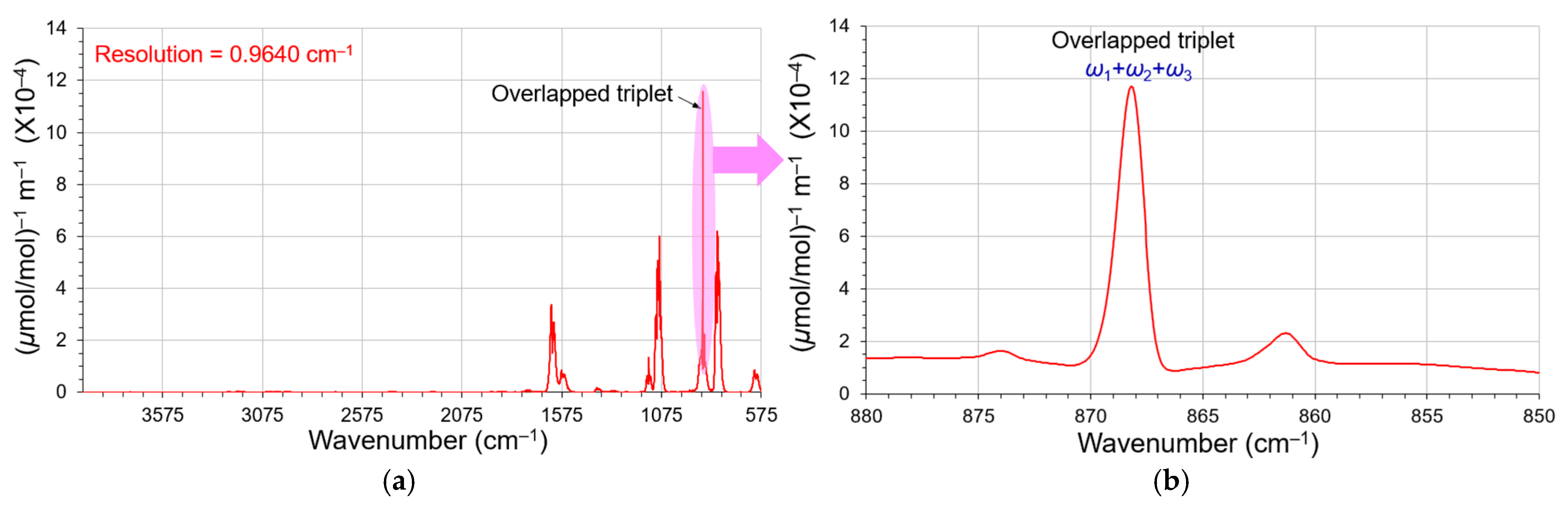
3.4. Deconvolution of the Closely Overlapped FT-IR Peaks

Because our approach is applicable to conventional FT spectroscopy, we also deconvoluted a FT-IR overlapping triplet in this section. 1,1-Dichloroethene is a major monomer used to manufacture polymer packaging material. Chu et al. acquired its high-quality FT-IR spectra in the NIST open FT-IR spectral source Quantitative Infrared Database [17]. Since the SNR of their spectral data is >1000, they are very desirable for our derivative deconvolution study. A FT-IR spectrum of 1,1-Dichloroethene vapor, as shown in Figure 13a, acquired on a Bruker IFS66V FT-IR spectrometer (Billerica, MA 01821, USA) at a resolution of 0.9640 cm⁻¹, was apodized by a 3-term Blackman–Harris window. This molecule exhibited a closely overlapped triplet related to its double-bond vibrations (868–869 cm⁻¹). We expanded this triplet in Figure 13b by adding 6 zero-fillings to render sufficient data points for its deconvolution. The broad bands underneath this triplet in Figure 13 were considered the spectral background in the following deconvolution.

The interferograms of gas phase FT-IR spectroscopy usually exhibit comparatively long and flat wings. After carefully evaluating the reproduced interferogram of 1,1-Dichloroethene, its decay coefficient was estimated to be 0.388 and yielded a FWHM = 1.243 cm⁻¹ in the frequency domain. Our reverse curve fitting approach quickly achieved good deconvolutions for the closely overlapped triplet and was profited by the superior SNRs of the FT-IR spectrum and their overlapping degrees 0.6 < γ < 0.9 (larger than 0.5). The deconvolution results are summarized in

Table 5. Deconvolution process and results of the closely overlapping triplet in Figure 10.

Peak		ω1	ω2	ω3
Overlapping γ		–	0.896	0.602
Cycle-0	cm−1	868.150	–	869.062
	A0	9.815 × 104	–	1.615 × 104
Cycle-1	cm−1	868.136	868.669	869.067
	A0	10.014 × 104	0.714 × 104	1.593 × 104
Cycle-2	cm−1	868.136	868.693	869.067
	A0	10.014 × 104	0.763 × 104	1.593 × 104
Filtered *	cm−1	868.134	868.686	869.062
	A0	10.005 × 104	0.763 × 104	1.593 × 104

* The filtered results (isolated by dismembering the other two peaks) are for information only.

. The reverse curve fitting results agree well with their filtered independent intensities. Their deconvolution details (Python codes and Excel demonstration) are specified in Section S3 of the Supporting Information.

Figure 14 presents a good comparison with the deconvoluted triplet (red spectrum), and its high-resolution spectrum (0.125 cm⁻¹, blue spectrum) obtained from the same database (apodized by a 3-term Blackman–Harris window) [17]. The deconvoluted peaks (ω₁, ω₂, and ω₃) are compatible with its high-resolution spectrum. The wavenumbers of the triplet in the high-resolution spectrum all shifted slightly higher (about +0.2 cm⁻¹).

4. Discussion

The PCM reverse curve fitting strategy carried forward good traditions in iterative operations and least-square algorithms for the quantitative deconvolutions from standard iterative least-squares fitting methods [26]. However, the iterative least-squares fitting procedures require either priori knowledge of the overlapping peaks or guessing their model parameters for the initial inputs, such as the peak shape, peak width, peak number and background, etc. The traditional methods only deal with simple background corrections. If an uncommon background did not appear in the blank sample and immersed underneath the overlapping band, it could cause the deconvolution iteration to fail to converge or incorrectly add the background into the fitted peaks.

Our new method uses partial curve matching on primary maximum portions of odd-order derivatives to imitate an independent peak in an overlapping band. The members of an overlapping band were gradually reduced to filter out an independent peak close to its real shape, not to fit the full spectral envelope with the proposed independent peaks. The PCM/dismembering approach therefore is a reverse curve fitting algorithm. We applied the curve fitting algorithm to deconvolute an overlapped peak to the time domain for its matched position, intensity, and width, and then performed FT to fit the peak as far as possible. The PCM procedure principally relies on D⁽³⁾ derivatives, or D⁽⁵⁾ potentially, since they have minimum derivative satellites [11]. The reverse curve fitting algorithm provides two kinds of measurements for peak intensities: PCM and filtered out. They should be almost identical when the deconvoluting process is convergent. Our algorithm can deconvolute the overlapping FT spectral bands either with the same peak width or with different FWHMs. The zero-cross points of third-order derivatives, D⁽³⁾, help locate the true peak position. The D⁽³⁾ primary maxima help find accurate peak height. The time domain signal decay coefficient and the filtered independent peak help determine peak width. Hilbert transform for a deconvoluted peak and linear regression help judge peak purity (see Figure 15 below) and the peak number in an overlapping band. The D⁽³⁾ primary maxima and the dismembering process support background corrections, as shown in the deconvolution of the Tetraphenyl porphyrin NMR overlapping band in Figure 12.

Many physical or chemical techniques can help resolve the overlapping peaks in NMR spectroscopy. The well-known procedures are spin decoupling, the nuclear Overhauser effect, solvent suppression, magic-angle spinning (solid NMR), and two-dimensional NMR spectroscopy [1] (pp. 105–119, 175–180). A notable subtraction is the “Add-to-Subtract” approach initiated by Ye et al. in 2012 for NMR analysis of metabolites [27]. The background in a biological sample can be effectively removed by comparing it with a second sample spiked with the known background. More advanced band-selective NMR pulse sequences developed by Alexandersson et al. in 2020 can selectively remove unwanted signals from dominant compounds [28]. Callon et al. recently obtained improvements in total line width up to 35% at a static magnetic field of 1.2 GHz with 160 kHz magic-angle spinning [29]. They successfully assigned almost two thirds of aliphatic protons of protein macromolecules in their high-resolution NMR studies. The deconvolution algorithms could provide further solutions in NMR analyses of biomacromolecules.

Overlapping triplets are highly recommended as fundamental paradigms to evaluate the efficiency and robustness of a deconvolution approach. We performed preliminary studies regarding methods of quantitative deconvolution of Group III overlapping triplets in FT spectroscopy. Our approach successfully deconvoluted real closely-overlapping triplets, and they could be difficult to deconvolute by other approaches. So far, the Huguenin and Jones algorithm is still the most effective method to locate overlapping peak positions [13]. We proceeded with the Huguenin and Jones algorithm to determine zero-crossing points of the consecutive odd-order derivatives. If a target peak is filtered precisely from its overlapping spectral band, the zero-crossing points should be homologues of its position as explicated by Equation (6), i.e., nearly the same. A matter of prime importance for a successful deconvolution is to identify the number of peaks in an overlapping band, more precisely, how many overlapped peaks exist above an analytical threshold. For FT spectroscopy, Marshall and Verdun presented a theoretical cycle of dispersion vs. absorption yielded by Hilbert transform to evaluate the “purity” of an isolated Lorentzian line [18] (pp. 11–12). The Hilbert transform of a deconvoluted peak can be used to test its “purity” in the deconvolution and help find the peak number in an overlapping band. The plot of ln[magnitude] versus time from the Hilbert transform of a single peak displays an extremely good linearity (R² = 0.9996) in Figure 15a, and the Hibert transform of a closely overlapping doublet in Figure 15b appears bent with a “poorer” value, R² = 0.9952. We can imitate a single peak and mix it with the similar background near the overlapping band and perform Hilbert transformation analysis to compare a deconvoluted peak with the single peak for their linearities under almost the same conditions. The poor linearity always indicates line-broadening, either from noise or overlapping peak(s).

Reverse curve fitting is an easy-to-use tool in the deconvolutions of FT spectroscopy and produces quantitative results. Of course, our new approach needs further refinement for more complicated overlapping scenarios, for example, deconvolutions of closely overlapped multiplets with asymmetric peak profiles, and how to better calibrate phase shifts in FT-NMR spectroscopy [30]. The facilitation of the deconvolutions depends largely on the overlapping degrees and noise level in an FT spectrum. Thus, we distinctively divided four overlapping scenarios as to their overlapping degrees. If the deconvolution only requires a qualitative resolution of the overlapping NMR peaks, it would be more convenient to use the odd-order derivative ratio algorithm developed in our previous work [11]. An analyst should select a suitable deconvolution approach and weigh the pros and cons according to concrete problems. It is better to test efficiency and reliability of a deconvolution method by comparing low- and high-resolution status. Eventually, highly accurate instruments are trustworthy whenever they are available [29].

5. Conclusions

Odd or even derivatives act as a key to decrypting the attributes of overlapping peaks. Our new approach overcomes the deconvolution barrier of overlapping degrees less than 1.0. We invested in the regular curve fitting algorithm for common overlapping FT bands without prior knowledge on solving their independent intensities. Our deconvolution approach using odd-order derivatives (D⁽³⁾ or higher) can deal with different peak widths, successfully applying deconvolutions of the closely overlapped triplets.

References

1. Richards, S.A.; Hollerton, J.C. Essential Practical NMR for Organic Chemistry, 2nd ed.; Wiley: Hoboken, NJ, USA, 2023. [Google Scholar]
2. Chu, X.; Huang, Y.; Yun, Y.-H.; Bian, X. Chemometric Methods in Analytical Spectroscopy Technology; Springer: Singapore, 2022. [Google Scholar]
3. Dubrovkin, J. Mathematical Processing of Spectral Data in Analytical Chemistry: A Guide to Error Analysis; Cambridge Scholars: Newcastle upon Tyne, UK, 2018. [Google Scholar]
4. Martinson, D.G. Quantitative Methods of Data Analysis for the Physical Sciences and Engineering; Cambridge University Press: Cambridge, UK, 2018. [Google Scholar]
5. Schmid, N.; Bruderer, S.; Paruzzo, F.; Fischetti, G.; Toscano, G.; Graf, D.; Fey, M.; Henrici, A.; Ziebart, V.; Heitmann, B.; et al. Deconvolution of 1D NMR spectra: A deep learning-based approach. J. Magn. Reson. 2023, 347, 107357. [Google Scholar] [CrossRef] [PubMed]
6. Li, D.-W.; Bruschweiler-Li, L.; Hansen, A.L.; Brüschweiler, R. DEEP Picker1D and Voigt Fitter1D: A versatile tool set for the automated quantitative spectral deconvolution of complex 1D-NMR spectra. Magn. Reson. 2023, 4, 19–26. [Google Scholar] [CrossRef] [PubMed]
7. Mathew, R.S.; Paluru, N.; Yalavarthy, P.K. Model resolution-based deconvolution for improved quantitative susceptibility mapping. NMR Biomed. 2024, 37, e5055. [Google Scholar] [CrossRef] [PubMed]
8. Wenchel, L.; Gampp, O.; Riek, R. Super-resolution NMR spectroscopy. J. Magn. Reson. 2024, 366, 107746. [Google Scholar] [CrossRef] [PubMed]
9. Venetos, M.C.; Elkin, M.; Delaney, C.; Hartwig, J.F.; Persson, K.A. Deconvolution and analysis of the 1H NMR spectra of crude reaction mixtures. J. Chem. Inf. Model. 2024, 64, 3008–3020. [Google Scholar] [CrossRef] [PubMed]
10. Sørensen, M.B.; Andersen, M.R.; Siewertsen, M.-M.; Bro, R.; Strube, M.L.; Gotfredsen, G.H. NMR-Onion—a transparent multi-model based 1D NMR deconvolution algorithm. Heliyon 2024, 10, e36998. [Google Scholar] [CrossRef]
11. Chen, S.-P.; Taylor, S.M.; Huang, S.; Zheng, B. Application of odd-order derivatives in Fourier transform nuclear magnetic resonance spectroscopy toward quantitative deconvolution. ACS Omega 2024, 9, 36518–36530. [Google Scholar] [CrossRef] [PubMed]
12. Callon, M.; Malär, A.A.; Pfister, S.; Římal, V.; Weber, M.E.; Wiegand, T.; Zehnder, J.; Chávez, M.; Cadalbert, R.; Deb, R.; et al. Biomolecular solid state NMR spectroscopy at 1200 MHz: The gain in resolution. J. Biomol. NMR 2021, 75, 255–272. [Google Scholar] [CrossRef] [PubMed]
13. Vandeginste, B.G.M.; De Galan, L. Critical evaluation of curve fitting in infrared spectrometry. Anal. Chem. 1975, 47, 2124–2132. [Google Scholar] [CrossRef]
14. Maddams, M.F. The Scope and Limitations of Curve Fitting. Appl. Spectrosc. 1980, 34, 245–267. [Google Scholar] [CrossRef]
15. Kauppinen, J.; Partanen, J. Fourier Transforms in Spectroscopy; Wiley-VCH: Berlin, Germany, 2001; pp. 14–16, 172. [Google Scholar]
16. Acorn NMR Inc. NUTS NMR Software, Demonstration version 20000813; Acorn NMR Inc.: Livermore, CA, USA, 2000.
17. Chu, P.M.; Guenther, F.R.; Rhoderick, G.C.; Lafferty, W.J. Quantitative Infrared Database. Also see: The NIST Quantitative Infrared Database. J. Res. Natl. Inst. Stand. Technol. 1999, 104, 59–81. Available online: https://webbook.nist.gov/chemistry/quant-ir/ (accessed on 19 September 2024). [CrossRef]
18. Marshall, A.G.; Verdun, F.R. Fourier Transforms in NMR, Optical and Mass Spectrometry: A User’s Handbook; Elsevier: Amsterdam, The Netherlands, 1990; p. 75. [Google Scholar]
19. Huguenin, R.L.; Jones, J.L. Intelligent information extraction from reflectance spectra: Absorption band positions. J. Geophys. Res. Solid Earth 1986, 91, 9585–9598. [Google Scholar] [CrossRef]
20. Gorkovskiy, A.; Thurber, K.R.; Tycko, R.; Wickner, R.B. Locating folds of the in-register parallel β-sheet of the Sup35p prion domain infectious amyloid. Proc. Natl. Acad. Sci. USA 2014, 111, E4615–E4622. [Google Scholar] [CrossRef] [PubMed]
21. Dubrovkin, J. Derivative Spectroscopy; Cambridge Scholars: Newcastle upon Tyne, UK, 2021; pp. 3–5, 18. [Google Scholar]
22. Kito, K. Digital Fourier Analysis: Advance Techniques; Springer: New York, NY, USA, 2015; pp. 105–119. [Google Scholar]
23. Wolberg, J. Data Analysis Using the Method of Least Squares: Extracting the Most Information from Experiments; Springer: Berlin/Heidelberg, Germany, 2006; pp. 34–36. [Google Scholar]
24. Reich, H.J. Spin-Spin Splitting: J-Coupling. 2017. UW-Madison. Available online: https://organicchemistrydata.org/hansreich/resources/nmr/ (accessed on 7 October 2024).
25. Shimizu, T.; Hashi, K.; Goto, A.; Tansyo, M.; Kiyoshi, T.; Matsumoto, S.; Wada, H.; Fujito, T.; Hasegawa, K.-i.; Kirihara, N.; et al. Overview of the development of high-resolution 920 MHz NMR in NIMS. Physica B 2004, 346/347, 528–530. [Google Scholar] [CrossRef]
26. O’Haver, T. A Pragmatic Introduction to Signal Processing with Applications in Scientific Measurement. July 2021. Available online: https://terpconnect.umd.edu/~toh/spectrum/CurveFittingC.html (accessed on 27 May 2025).
27. Ye, T.; Zheng, C.; Zhang, S.; Gowda, G.A.N.; Vitek, O.; Raftery, D. “Add to Subtract”: A simple method to remove complex background signals from the 1H nuclear magnetic resonance spectra of mixtures. Anal. Chem. 2012, 84, 994–1002. [Google Scholar] [CrossRef] [PubMed]
28. Alexandersson, E.; Sandstrom, C.; Lundqvist, L.C.E.; Nestor, G. Band-selective NMR experiments for suppression of unwanted signals in complex mixtures. RSC Adv. 2020, 10, 32511–32515. [Google Scholar] [CrossRef] [PubMed]
29. Callon, M.; Luder, D.; Malär, A.A.; Wiegand, T.; Římal, V.; Lecoq, L.; Böckmann, A.; Samoson, A.; Meier, B.H. High and fast: NMR protein–proton side-chain assignments at 160 kHz and 1.2 GHz. Chem. Sci. 2023, 14, 10824–10834. [Google Scholar] [CrossRef] [PubMed]
30. Lee, J.P.; Comisarow, M.B. The phase dependence of magnitude spectra. J. Magn. Reson. 1987, 72, 139–142. [Google Scholar] [CrossRef]
Figure 1. A single 1H NMR peak (blue spectrum) imitated at chemical shift 7.0 ppm. The peak center coincides with the zero-crossing points of its 3rd-order derivative D(3) (brown line) and 5th-order derivative D(5) (pink line).
Magnetochemistry 11 00050 g001
Figure 2. A close overlapping triplet (blue spectrum) simulated from three independent peaks (dotted brown peaks ω2, ω3, and ω4) as the parameters specified in the right. Peak ω1 is well separated from the triplet and used as a reference peak.
Magnetochemistry 11 00050 g002
Figure 3. (a) A white Gaussian noise was added into the simulated spectrum of Figure 1 at SNR = 20:1. The amplified noise by D(3) overwhelmingly dominates the derivative spectrum (solid brown line against secondary axis at the right side). (b) After denoising, the recovered D(3) spectrum (solid brown line against the right secondary) compared with its authentic D(3) depicted in green dashed line. The decay coefficient of the spectral signal will be determined next by cutting the triplet off along a red dashed line at its baseline to isolate the reference peak ω1.
Magnetochemistry 11 00050 g003
Figure 4. The Hilbert transform analysis (pink line) for reference peak ω1 isolated from Figure 3b after removing the apodization window. The upper-half part is linear (dashed blue line; R2 = 0.989) with a slope = −627.260 (s−1), with the noise residues in the lower-half part.
Magnetochemistry 11 00050 g004
Figure 5. Illustrations of PCM process. The denoised raw spectrum is depicted in solid blue, its derivative D(3) in solid brown, the matched independent peak by the light blue dashed line, and the matched peak by the dotted brown line. (a) An independent peak was imitated to match the left D(3) primary maximum portion (red spots) of reference peak ω1 and used as a reference standard in the quantitative deconvolution of the closely overlapped triplet. (b) The D(3) right primary maximum of back edge peak ω4 of the triplet was matched partially with D(3) (red spots) of an imitated independent peak. (c) The D(3) right primary maximum of front edge peak ω2 was matched partially (red spots) by an imitated independent peak after the matched ω4 was removed from the raw spectrum (dismembering). (d) After rematching edge peak ω4 by dismembering the matched ω2, the middle peak ω3 was filtered out and displayed a clear D(3) derivative. The filtered ω3 was then matched by an imitation peak ω3 to estimate its initial peak position and intensity. We hereinafter can perform the reverse curve fitting procedure to individually deconvolute each peak in the triplet.
Magnetochemistry 11 00050 g005
Figure 6. The deconvolution process of the closely overlapped triplet. %Deviation of front edge peak ω2 is depicted in blue line; middle peak ω3 in brown; and back edge peak ω4 in green. The edge peak ω4 approached the best result in Cycle-3 (appraised by relative residue analysis). The quantitative deconvolutions were achieved in Cycle-4 and afterward for the other two peaks.
Magnetochemistry 11 00050 g006
Figure 7. Relative residue analyses of dismembering Cycle-4 (dashed brown line) against Cycle-3 (blue line) for back edge peak ω4. Its deconvoluted intensity in Cycle-3 achieved the best result (residue% = 0.175%). The residue analysis helped to optimize the reverse curve fitting.
Magnetochemistry 11 00050 g007
Figure 8. An absorption-mode 300 MHz NMR spectrum of Ethylbenzene. The spin–spin coupling of its aryl protons exhibited two merged bands (blue spectrum). A sharp peak ω1 from solvent Chloroform-d displayed a narrower peak width than the other aryl proton peaks. The ortho- and para-proton band will be removed along the dashed brown line to reduce their overlapping effects for deconvolutions of residue solvent ω1 and the meta-proton peaks (ω2, ω3, and ω4).
Magnetochemistry 11 00050 g008
Figure 9. The aryl proton NMR spectrum (blue spectrum) after striking the ortho- and para-proton band from Figure 7. The front edge peak ω4 was imitated by a PCM ω4 peak (dashed pink) with its D(3) derivative (brown spectrum) for evaluation of its peak position, width, and amplitude simultaneously. The D(3) primary maximum of the ω4 was well matched by the PCM D(3) (dashed green).
Magnetochemistry 11 00050 g009
Figure 10. A “leaning” meta-proton triplet (blue spectrum) restored after dismembering the solvent peak ω1 (dashed gray peak). A tiny unknown peak at 7.195 ppm is indicated by a green arrow. The deconvoluted meta-proton triple with equal spacings is depicted in pink.
Magnetochemistry 11 00050 g010
Figure 11. An absorption-mode 400 MHz NMR spectrum of Tetraphenyl porphyrin. The spin–spin coupling of its ortho phenyl protons exhibited a broad overlapping band (blue spectrum). The zero-crossing points of the D(3) derivative (brown spectrum) indicated by gray lines are very clearly observed. There should be at least 10 overlapping peaks in this band.
Magnetochemistry 11 00050 g011
Figure 12. The gray profile is the original overlapping band. The deconvoluted independent peaks of the 10 overlapping peaks (depicted in various colors other than gray and red) with their background (red spectrum). Peaks #4, 5, and 6 are closely overlapped with the background.
Magnetochemistry 11 00050 g012
Figure 13. (a) FT-IR spectrum (red) of 1,1-Dichloroethene adopted from the NIST Quantitative Infrared Database at a resolution of 0.9640 cm−1 [17]. A large closely overlapped triplet (shaded pink) appeared at 868 to 869 cm−1. (b) This triplet was expanded and reproduced by adding 6 zero-fillings. The broad peaks underneath the triplet were treated as the background in the deconvolution process.
Magnetochemistry 11 00050 g013
Figure 14. The deconvoluted triplet (red spectrum) of 1,1-Dichloroethene compared with its high-resolution spectrum at a resolution 0.125 cm−1 (blue spectrum). The high-resolution spectrum was scaled down to match the intensity exhibition.
Magnetochemistry 11 00050 g014
Figure 15. (a) Hilbert transform analysis (pink line) of a single peak without noise and apodization. The linear regression (dashed blue line) on its main body is extremely good (R2 = 0.9996). (b) The Hilbert transform analysis (pink line) of a closely overlapped doublet appear bent away from its trendline (dashed blue line). Its R2 dropped to 0.9952.
Magnetochemistry 11 00050 g015