


Abstract
The origin of homochirality by rotational magnetoelectrochemistry was theoretically examined. Electrochemical reductions in a rotating solution under a static vertical magnetic field were concluded to yield microscopic vortices with L-activity for enantiomeric reagents, whereas D-active vortices arise from electrochemical oxidation. The reduction case was experimentally verified by rotational magnetoelectrodeposition (RMED) of copper films using an electrolysis cell rotating in a magnetic field, where L-active screw dislocations were created by L-active microscopic vortices. In all the cases of the directions of magnetic polarity and system rotation, the RMED films exhibited L-activity for the enantiomeric reactions of amino acids.
1. Introduction
Chirality is one of the fundamental issues in biochemical systems, where a number of chemical reactions are controlled by chiral stereoselectivity, and symmetry-breaking in chirality concerning the birth of life has long intrigued many scientists. Chiral symmetry breaking occurs when a physical or chemical process that does not have a preference for the production of one or the other enantiomer spontaneously generates a large excess of one of the two enantiomers: lefthanded (L) or righthanded (D). From the energetic point of view, these two enantiomers can exist with an equal probability, and inorganic processes involving chiral products commonly yield a racemic mixture of both (L) and (D) enantiomers. However, life on earth utilizes only one type of amino acids and only one type of natural sugars: (L)-amino acids and (D)-sugars [1].
One of the most interesting questions in the molecular evolution towards the birth of life is how the biological system selected one enantiomer of a chiral biomolecule. To identify possible external influences on such a selection, various mechanisms have been proposed, such as circularly polarized light [2,3,4], magneto-chiral fields [5], vortex and stirring conditions [6,7,8], nonlinear autocatalysis [9,10], gravitational effect [11], and combinations of external fields [12]. However, which one is chosen, D- or L-activity, still depends on the accidental nature.
Fluid flow, such as vortex motion, could also be one of the most probable symmetry-breaking factors. Kondepudi et al. reported that solution stirring breaks the racemic state in the crystallization of enantiomorphous NaClO3 [6]. Ribo et al. reported that mechanical vortices induce chirality in the aggregation of achiral porphyrins in aqueous solutions [7]. These facts demonstrate that macroscopic vortices have an asymmetric influence on crystallization and aggregation at the nanometer scale.
Furthermore, under the prebiotic oceans on the early Earth, surfaces of minerals could serve as catalysts in the formation of amino acids [13,14]. If such catalytic surfaces were chiral, the chiral symmetry would be broken for the enantiomers of amino acids, and one-handed amino acids would become dominant. It is a crucial point for the formation of a homochiral biosystem whether the minerals have chiral surfaces or not. Thus, studies of chiral surface formation in deposition and crystal growth processes are important to explore the origin of life.
According to F. C. Frank et al. [15,16], a crystal surface has numerous screw dislocations, of which steps spirally proceed with the addition of atoms or molecules as the sites of growth. As exhibited by STM observation, in electrodeposition also, a lot of screw dislocations emerge on the growing surfaces [17], and the center of a screw dislocation has a typical chiral structure, which could serve as a chiral catalyst. As will be shown below, in electrodeposition under a vertical magnetic field, Lorentz force induces microscopic magnetohydrodynamic (MHD) vortices, which control the formation of chiral screw dislocations, adding chiral activities to the deposit surface. As discussed in Appendix E, the MHD vortices may bias or enhance existing tendencies rather than solely cause such structures.
In an electrode reaction under a vertical magnetic field, a tornado-like macroscopic rotation called a vertical magnetohydrodynamic (MHD) flow (VMHDF) appears over the electrode [18,19,20,21]. Under the rotation, numerous microscopic vortices emerge so that as shown in Figure 1, the electrodeposition under a vertical magnetic field (magnetoelectrodeposition, MED) proceeds with vortices of characteristic sizes in accordance with the nucleation in three generations; in the 1st generation, 2D nucleation with micro-MHD vortices of a representative size of 10−4 m, and in the 2nd generation, 3D nucleation with nano-MHD vortices of a size of 10−7 m, and finally in the 3rd generation, screw dislocation with ultra-micro-MHD vortices of 10−10 m. All the generations form a nesting box structure so that micro-MHD vortices result from VMHDF, nano-MHD vortices from micro-MHD vortices, and ultra-micro-MHD vortices from nano-MHD vortices [18,19]. The direction of VMHDF depends on the magnetic field polarity. Hence, the chiral sign of the deposit surface becomes opposite when the magnetic field is reversed, representing odd chirality for magnetic field polarity [20]. The precessional rotation from higher generation is transmitted to lower generation through the instability processes of nucleation so that the resultant chiral activities are sensitive to the electrochemical conditions of each nucleation process. Consequently, the enantiomeric activity of the deposit surface varies not only with the direction of the magnetic field but also in the presence of electrochemical additives, such as chloride ions [21].
Figure 1.
The three-generation model of electrodeposition under a VMHDF (MED). : magnetic flux density, VMHDF: vertical MHD flow. Reprinted from Refs. [18,19].
In an electrochemical reaction under a magnetic field, an inviscid layer of ionic vacancies is formed on the electrode surface [22,23]. Ionic vacancies are produced from the conservation of linear momentum and electric charge in the charge transfer during an electrode reaction [24,25]. Unstable embryo vacancies immediately after their creation are rapidly stabilized by solvation and develop into solvated vacancies surrounded by ionic clouds. Figure 2 exhibits the schematics of solvated negative and positive ionic vacancies yielded at the cathode and the anode, respectively. The solvation energy of the ionic cloud is used for the expanding work of the vacancy core, saving the energy in it, so that an ionic vacancy behaves as an iso-entropic particle without entropy production. Therefore, ionic vacancies do not interact with other solvent molecules, keeping a natural lifetime of 1 s [26,27], which is extraordinarily longer than a thermal collision period of 10−10 s. This means that an ionic vacancy acts as an atomic-scale lubricant and that the vacancy layer behaves like an inviscid fluid. Due to quite a high Reynolds number, the microscopic vortices could not rotate in a usual solution but rotated in or on a vacancy layer.
Figure 2.
Solvated ionic vacancies [25,26]. Partially polarized charges of water molecules surround the free spaces. (a) Negative vacancy. (b) Positive vacancy. H: proton, O: oxygen atom, : positive partial polarized charge, : negative partial polarized charge, ⊕: cation, ⊝: anion. Reprinted from Refs. [18,19].
Under a vertical magnetic field, microscopic anticlockwise (ACW) and clockwise (CW) MHD vortices arise on and in a vacancy layer, which cannot be discriminated as they are. However, as shown in Figure 3a, to conserve local angular momentum and mass, we can assume a pair of vortices rotates, in opposite directions with upward and downward flows. As a result, the combination of the vortex pair is limited to two cases, i.e., ACW and CW vortices with upward and downward flows or downward and upward flows, respectively [18,19]. As shown in Figure 3b,c, an upward vortex sucks up and gathers ionic vacancies, whereas a downward one drives them away, so that the former rotates on the free surface covered with ionic vacancies and the latter rotates on the exposed rigid surface. Furthermore, as shown in Figure 4, because the active reaction sites among ionic vacancies rotate with a free-surface vortex (FV), any chirality would not take place. Chiral reaction product such as chiral screw dislocation is thus expected only by a rigid-surface vortex (RV) rotating against stationary active sites.
Figure 3.
Pair formation of microscopic MHD vortices on the electrode surface [16,17]. (a) Pair formation of upward anticlockwise (ACW) and downward clockwise (CW) vortices. (b) An upward free-surface vortex (FV). (c) A downward rigid-surface vortex (RV). Light orange sphere: ionic vacancy.
Figure 4.
Formation of screw dislocations by microscopic vortices. (a) The case of rigid-surface vortex (RV). (b) The case of free-surface vortex (FV). The RV relatively rotates against the active points fixed on the rigid surface, whereas the active points on the free surface covered with a vacancy layer rotate with the FV without any relative motion. Chirality, therefore, occurs only for the RV.
Figure 5 shows a screw-dislocation-like deposition theoretically calculated for 3D nucleation formed by a clockwise (CW) nano-MHD vortex on the rigid surface in the 2nd generation [19]. Though much larger scale of length than actual screw dislocation, the same CW chirality as the micro-MHD vortex appears. This result indicates that chiral screw dislocations are created by ultra-micro MHD vortex flows on the rigid surface with the same chirality, which would be generalized as a fact that a chiral nucleus is created by a corresponding chiral vortex on the rigid surface. If unrelated to electrode reactions, chiral vortices were made, and we could control the chiral activity of a deposit surface by the external physical parameters, including a magnetic field.
Figure 5.
Calculated 3D nucleus with CW chirality arising from downward CW vortices on the rigid surface in the 2nd generation [19], which looks like a screw dislocation. : magnetic flux density shown by a green arrow. The yellow line and red curve indicate the directions of the downward flow and vortex rotation. Reprinted from Ref. [19].
As discussed above, for controlling chiral microscopic vortices unrelated to chemical or electrochemical conditions, it is insufficient to use only a magnetic field as an external physical parameter. We therefore introduce a new physical parameter, the angular velocity of system rotation. As will be shown later, by using such two parameters, we succeeded in producing the microscopic MHD vortices with controlled chirality.
The theoretical outline of the present paper is therefore provided as follows; we first assume an electrolysis system without a VMHDF under a vertical magnetic field, where only microscopic vortices called MHD vortex flows are induced by the Lorentz force fluctuation, and to conserve local angular momentum and mass, a pair of neighboring vortices appear, rotating each other in the opposite directions. We then apply a horizontal rotation to the system, thereby imposing the Coriolis force on the vortices to induce precession. As a result, from the balance between the Lorentz force and the Coriolis force, either of the vortex pairs tends to stop rotation so that the other can select the precession from the system rotation. As a result, independent of the directions of the magnetic field and rotation, only a pair of ACW and CW vortices on the rigid and free surfaces is permitted, respectively. Since chirality arises only from the rigid-surface vortices, in the case of rotational magnetoelectrodeposition (RMED), L-active, ACW screw dislocation would be obtained. If an enantiomeric reagent had the sensitivity for vortex rotation, an L-active reaction would be predominant. The experimental validation is presented by the chiral activity of copper RMED. Therefore, the theoretical procedure will be taken in accordance with the case of RMED.
2. Theory
2.1. Basic Equations
First, we explicitly consider an inertial frame with a static magnetic field. In this frame, a coordinate system (x, y, z) defined for an electrolysis cell containing a planar electrode on the x-y plane, rotates with the cell at an angular velocity (s−1) around the z-axis (see Figure 6). As will be shown later, in the present case, we assume that the electrolysis current flows perfectly parallel to the magnetic field so that a tornado-like macroscopic rotation (VMHDF) arising from the macroscopic distortion of current lines does not occur [22].
Figure 6.
The coordinate system of rotational magnetoelectrochemistry. The electrode surface agrees with the x-y plane, so that the areas and are defined as solution- and electrode-phases, respectively. : magnetic flux density vector, : rotational vector, : current density vector.
As shown in Appendix A, the overall current density (A m−2) flows under a magnetic flux density (T, tesla), so that the Lorentz force per unit mass, i.e., acceleration (m s−2) is generated in the following,
In addition, an observer at rest in the rotating system recognizes two kinds of forces, i.e.,
where is rotational force per unit mass, i.e., acceleration (m s−2), is the vector of angular velocity (s−1), is the vector of velocity (m s−1), and is the vector of position (m). The first and second terms on the right-hand side represent the Coriolis force and the centrifugal force.
Then, we consider an incompressible fluid at a uniform temperature so that the basic equations are given in the following: the momentum equation is first in tensor notation,
where is the velocity component (m s−1) (i = 1, 2, 3), and the coordinate (m) is expressed by implies , and is the magnetic permeability (4 N A−2). and are the kinematic viscosity (m2 s−1) and the density (kg m−3), respectively. is Levi Civita symbol (transposition of tensor). In view of an incompressible fluid, the continuity equation is fulfilled.
If a fluid element has a velocity , the electric field it will experience is not (V) as measured by a stationary observer, but . In an electrolytic solution, the electricity is carried by the diffusion as well as conductivity of ionic species so that the current density will be given by
where is defined by is the electrical conductivity (S m−1) defined by
where is the signed charge number, is the mobility (m2 V−1 s−1), F is the Faraday constant (96,500 C mol−1), is the molar concentration of ionic species i (mol m−3), and is the diffusion constant (m2 s−1).
Applying Equation (A10) to Maxwell’s equations, Equations (A1)–(A3), in Appendix A, we finally obtain the equation of magnetic flux density in tensor notation.
where is the resistivity (magnetic viscosity) (m2 s−1) defined by
Finally, the mass transfer equation of metallic ion is expressed by the concentration and diffusion coefficient .
2.2. Equations of the Nonequilibrium Fluctuations
As discussed in Appendix B, we simply consider an infinite horizontal layer of fluid in a state of uniform rotation with an angular velocity and subject to a uniform magnetic flux density. Here, we shall restrict our discussion of this problem to the case when and act in the same vertical direction. In addition, the current density also works in the vertical direction. Considering that a vector of rotation is an axial vector, we write down the following notation.
As a result, for each generation of nucleation, we obtain the fluctuation equations.
where and are the z-fluctuation components of the magnetic flux density (T) and the current density (A m−2). and are the z-components of the fluctuations of the velocity (m s−1) and the vorticity (s−1).
The concentration of the metallic ion is expressed as
where and are the molar concentration in the absence of fluctuation (mol m−3) and the concentration fluctuation (mol m−3), respectively. Mass transfer equation, Equation (A18), is also rewritten as
is the average concentration gradient of the metallic ion in each generation of nucleation (mol m−4). It takes different values depending on the generations; the concentration gradient of the 1st generation is formed in the diffuse layer of the electric double layer, that of the 2nd generation is defined by the diffusion layer, and in the 3rd generation, it is formed in front of screw dislocations. However, because they are connected in series, assuming that their formations are controlled by the mass transfer in the diffusion layer of the 2nd generation, we can simply describe their expressions by the ratio of the concentration difference (mol m−3) against the average diffusion layer thickness (m) in the following:
is defined by
where and are the bulk and surface concentration (mol m−3) of the metallic ion, respectively.
2.3. Amplitude Equations of the Fluctuations
For the fluctuations, we assume the following 2D plane waves.
where ‘i’ is the unit imaginary number. , , , and are the amplitudes of the fluctuations, and and are the wavenumbers (m−1) in the x- and y-directions, respectively.
Substituting Equations (C1a)–(C1e) into Equations (B17a)–(B17d) and (B19), and assuming that the fluctuations are at a quasi-steady state, we obtain
where and . Substituting Equation (C3b) into Equation (C3c), and using the resistivity in Equation (A15), we obtain
where and imply the magneto-induction coefficient (m−2) and Coriolis force coefficient (m−2), expressed as
and
Then, substitution of Equation (C3a) into Equation (C3d) leads to
Introducing a representative length d (m), we have Tayler number.
In addition, the nondimensional form of is given by
Both hand sides of Equation (C4a) are multiplied with , and Equation (C5) is substituted into the resultant equation, so that we derive the final equation to solve.
Equations (C5) and (C7) with Equation (C3e) are solved under the following conditions.
2.4. Boundary Conditions of the Fluctuations on the Rigid and Free Surfaces
The fluid of the solution is confined between and . Regardless of the nature of these boundary surfaces, we must first require that the vertical velocity be zero.
where the condition for also means
At the electrode surface , as shown in Figure 3, two types of vortices rotate on the rigid and free surfaces. Accordingly, we distinguish two types of hydrodynamic boundary surfaces.
2.4.1. Rigid Surface on Which No Slip Occurs
The conditions that no slip occurs on this surface imply that not only w, but also the horizontal x- and y-components of the velocity u and v (m) vanish.
These conditions must be satisfied for all x and y on the surface, so that for the rigid surface, we obtain
Substituting Equation (1b) into the equation of continuity in Equation (A9), we can derive the boundary condition of
The normal component of the vorticity is defined by
From Equations (3b) and (5), we obtain the boundary condition of .
2.4.2. Free Surface Where No Tangential Stress Acts
The conditions on a free surface are that the stress tensors are zero, i.e.,
where and are the viscous stress tensor (Pa):
and
where is the viscosity (Pa s). Substitution of Equation (1b) into Equation (7) leads to
Differentiating the equation of continuity in Equation (A9) regarding z, and substituting Equation (8c) into the resulting equation, we finally get the boundary condition of .
Then, after the differentiation of Equation (5) with respect to z, substituting for Equation (8c) in the resulting equation, we have
We also add the following condition.
In addition to these pure hydrodynamic conditions, we can write down the other conditions concerning mass transfer. From Fick’s first law, we have the following relationship between the fluctuations of the current density and concentration
together with the conditions
Based on the above discussions, the boundary conditions of the amplitudes are summarized as follows.
and either
or
2.5. General Solution of
First, to obtain the general solution of in Equation (C7), as shown in Appendix D, the following function form is assumed.
For the condition , mainly follows , which is expressed by a series of z.
where , are the arbitrary quasi-static constants, which are functions of t.
Substituting Equation (D1) into Equation (C7), we finally derive the following equation.
Equation (D6) must be an identity with regard to z, so that each i-th term is equal to zero.
where the parameters to are given by Equation (D5b) in Appendix D.
2.6. Solutions of on the Rigid and Free Surfaces and
Though Equation (D7) has an infinite number of coefficient , as will be shown, the boundary conditions require only three coefficients, i.e., , and . To derive the exact value of each , the contribution of the higher-order coefficients must be considered. In the present case, however, in view of the series converging to zero, we make an approximation that the higher order contribution i = 2 is represented by itself.
In accordance with such a scheme, putting for in Equation (D7), we get the simplified relationship between the coefficients of the general solution of .
where from Equation (D5b),
Under the condition Equation (18a), from Equation (D1), should be solved as
2.6.1. Amplitude of the Vorticity Fluctuation on the Rigid Surfaces
The vorticity induced by the system rotation and magnetic field on the rigid surfaces follows the boundary condition Equation (17a). To derive the expression of on the rigid surface, substituting Equation (19) into Equation (17a), we first obtain
Then, inserting Equation (20) into Equation (18a), we get the following relationship.
where is the vorticity coefficient of the rigid surface.
where subscript ‘r’ implies the rigid surface. Substitution of Equations (20) and (21) into Equation (19) leads to the amplitude of the vorticity fluctuation on the rigid surfaces.
2.6.2. Amplitude of the Vorticity Fluctuation on the Free Surfaces
The vorticity on the free surfaces follows the boundary condition Equation (17b). Substituting Equation (19) into Equation (17b), we have
Replacing from Equation (18a) with in Equation (24), we get
where is the vorticity coefficient of the free surface.
where subscript ‘f’ implies the free surface. Substituting Equations (24) and (25) into Equation (19), we obtain the amplitude of the vorticity on the free surfaces.
2.7. General and Special Solutions of the Amplitude of the Velocity Fluctuation
In accordance with the usual differential equation theory, in Equation (C5) is decomposed to the general solution and the special solution so that they will be separately solved in the following.
2.7.1. The General Solution
satisfies the following equation.
In the same way as for in Equation (D1), the function form is assumed as
and is expressed as
where , , , are the arbitrary coefficients of the general solution, which are functions of .
With Equations (29) and (30), in accordance with Equation (D3b), Equation (28) is expanded by the operator D.
Then, from Equation (D3a), the following equation is derived.
Though Equation (32) has infinite number of coefficients, as will be shown later, the boundary conditions require only three coefficients , , and . However, to derive the exact value of , the contribution of higher order coefficients , , than must be considered. Considering that they form a series converging to zero, we make an approximation that the higher order coefficients than is represented by . Due to the identity concerning z, each term of in Equation (32) is equalized to zero.
For we have
For , we get
From Equations (33a) and (33b), the terms of are eliminated, so that we finally obtain the equation of , and .
2.7.2. The Special Solution
As for the special solution , Equation (C5) leads to the equation.
According to Equation (29), is also written by
where is expressed as
where , , , are the arbitrary coefficients of the special solution, which are functions of .
From Equations (D3a) and (D3b), we have the right-hand side of Equation (35) as a series of z.
Using Equations (D3a), (D3b) and (36), we can expand the left-hand side of Equation (35) with regard to z.
Substituting Equations (38) and (39) into Equation (35), and comparing each term with the same power of z, we can pick up the following equations.
For
For
For
Therefore, from Equation (40c), the coefficient is given by
Substituting Equation (41a) into Equation (40b), is expressed by and
Inserting Equations (41a) and (41b) into Equation (40a), is represented by , and
2.8. Solutions of the Rigid- and Free-Surface Amplitudes and
The solution of is expressed as
Then, from Equations (29) and (30), the general solution is provided by
with the coefficient equation, Equation (34).
On the other hand, from Equations (36) and (37), the special solution is written by
Since the solution of is composed of the sum of the general solution and the special solution we have the following relationship between their coefficients.
Substituting Equation (45) into Equation (34), we derive the following equation.
Under the condition of Equation (46), the solutions on the rigid and free surfaces are derived.
2.8.1. The Rigid-Surface Solution
From the general boundary condition for a solid surface, for z in Equation (15), we have
For the rigid surface, the boundary condition for z in Equation (17a) is fulfilled, so that substituting Equation (42) into Equation (17a) and inserting Equation (47) into the resulting equation, we obtain
Here, the rigid-surface conditions of the vorticity were derived by in Equation (20) and in Equation (21). Equations (47) and (48) are first substituted into Equation (46), then together with Equations (20) and (21), Equations (41a)–(41c) are inserted into the resulting equation, so that we finally get
To describe the equation in Equation (49a) more explicitly, under the electrochemical condition , using Equation (22), we rewrite Equation (49a) as follows.
The relationship is generally obtained in any electrochemical system from the low electric conductivity of electrolyte solution and the scale of length of nucleation , i.e., and are obtained.
In view of Equations (47) and (48), is expressed as
2.8.2. The Free-Surface Solution
In addition to the condition in Equation (47), from the free-surface condition for z in Equation (17b), we have
As for the coefficients of the vorticity, it follows that in Equation (24) and in Equation (25) are derived for the free-surface case. Using Equations (47) and (51) together with Equations (24) and (25), in the same way as Equation (49a) in the rigid-surface case, we obtain
Furthermore, under the electrochemical condition , with Equation (26), we rewrite Equation (52a) as follows.
Finally, in view of Equations (47) and (51), is written as
2.9. Solutions of the Amplitudes of the Rigid- and Free-Surface Concentration Fluctuations and
The solution of the concentration fluctuation amplitude is also described by the sum of the general solution and the special solution .
From Equation (C3e), the general solution satisfies
Applying the boundary condition Equation (14),
we get
where is an arbitrary constant as a function of t.
Then, the special solution is differently solved for the rigid and free surfaces.
where and are the rigid- and free-surface velocity amplitudes in Equations (50) and (53), respectively. is the mass transfer coefficient (mol s m−6) defined by the average concentration gradient in the diffusion layer and the diffusion coefficient .
changes the sign with , which is positive for a cathodic reaction, and negative for an anodic reaction.
2.9.1. The Rigid-Surface Solution
Equation (57) is solved for the rigid-surface as follows.
The solution of the rigid-surface is therefore expressed by the sum of Equations (56) and (59).
The derivative is given by
2.9.2. The Free-Surface Solution
Equation (57) is solved for the free-surface case as follows.
The solution of the free-surface amplitude is written by the sum of Equations (56) and (61).
The derivative is
2.10. Vortex Filter Functions on the Rigid and Free Surfaces and
As has been shown in the previous papers [16,17], the nonequilibrium fluctuations in magnetoelectrodeposition (MED) under a VMHDF are described by their amplitude factors, and according to the amplitude factor, they exponentially develop with time in the unstable case, and dwindle in the stable case. An amplitude factor is composed of the product of two parts; one is a vortex filter function, where wavenumber components necessary for the electrode reaction are selected from the solution-side fluctuations through MHD vortex rotations, whereas the other corresponds to the electrode reaction process, such as electrodeposition, utilizing the selected components. As a result, if the vortex motions were prohibited, the amplitude factor would converge to the one in a static solution without a magnetic field and system rotation. This means that to describe the vortex behaviors in the solution, it is sufficient to examine the vortex filter function. In the following, for examining the role of the chiral vortex motions in magnetoelectrochemical reactions in a rotating system, we pick up the filter function.
Whether rigid or free, from Equation (C3c), the following relationship among the amplitudes of the vorticity , velocity and current density is derived.
where is defined by Equation (C4c), and is the MHD coefficient (T m s kg−1) expressed by
In view of the fact that the fluctuations vanish at a distance far away from the surface together with Equation (15), we have
To deduce the amplitude for i.e., of the current density fluctuation on the rigid and free surfaces, Equation (63a) is integrated with regard to z from to . Using the boundary conditions Equations (64a) and (64b), we obtain the integrated equation
Since using the formulas on in Equations (D3a) and (D3b), we obtain the equation of
we can calculate the following integration.
Substituting Equation (67) into Equation (65), we get
From the boundary condition of the current density fluctuation Equation (16), we have
Substituting for from Equation (68) in Equation (69), we obtain the boundary condition of related with the vorticity, which is separately solved for the rigid- and free-surface cases.
2.10.1. Rigid-Surface Vortex (RV) Filter Function
Inserting Equation (21) into Equation (70), and using the resultant equation and Equations (22) and (49b), we rewrite Equation (60b) at the rigid surface as a rigid-surface boundary condition.
where
and
Here, for simplicity, assuming the electrochemical condition from Equations (49b), (60a), (60b) and (71a), we get another rigid-surface boundary equation, i.e.,
To obtain the RV filter function selecting proper fluctuation components through the rigid-surface vortices, we divide Equation (71a) by Equation (72), obtaining , which is expressed by the following fractional expression of the denominator function and the numerator function [16,17].
where and are expressed as
and
2.10.2. Free-Surface Vortex (FV) Filter Function
Inserting Equations (24) and (25) into Equation (70), and using the resultant equation with Equations (26) and (52b) under the electrochemical condition , from Equation (62b), we can derive a free-surface boundary condition.
Then, using the same electrochemical condition for Equation (26), we can rewrite Equation (62a) as another free-surface boundary condition.
The FV filter function of the rigid-surface vortexes is thus defined by
where and are expressed as
and
When the system rotation is stopped, , i.e., is inserted into Equations (73a) and (75a), so that we get the filter functions , which are equal to those of the stationary solution [18].
2.11. Precessional Conditions of the Microscopic RMHD Vortices
To distinguish MHD vortices in a rotating system from those in a stationary system, we especially call the former vortices as rotational MHD (RMHD) vortices. For an RMHD vortex to contribute to a chiral reaction process such as chiral nucleation, some interaction between the vortex and the mass flux of the reagents is required. However, due to the nature of axial vector, the z-component of the vorticity vector induced by a vertical magnetic field rotates horizontally along the x-y plane, and therefore does not make interplay with the mass flux vector having only z-component (see Figure 6). The system rotation bestows precessional motion on the vorticity vectors to interact with the mass flux vector. This means that to assess the mechanism correctly, the roles of not only the vorticity itself, but also the system rotation, must be examined.
A new quantity describing the precessional motions, i.e., Coriolis vorticity (m−2 s−1) is thus introduced.
where is a scalar quantity shown in Equation (C4c), so that is the same axial vector as . The rotational direction of an RMHD vortex is not determined by the sign of , but by the sign of
Using the Coriolis vorticity, we can rewrite the z-component of the velocity in Equation (B17d).
As shown in Equation (77), the z-component of the velocity, receives precessional motion by , controlling the mass transfer for chiral deposition. In a stationary system, as has been discussed in the preceding papers [18,19], a precessional motion transfers from the 1st generation to the 3rd generation indirectly through MHD vortex rotations in each generation. However, in the present case, it is directly donated to all the vortices by the system rotation without any contribution of electrochemical reactions.
In the same way as ordinary vorticity , the Coriolis vorticity determines the rotational directions of RMHD vortices; the positive and negative values of indicate anticlockwise (ACW) and clockwise (CW) rotations, respectively. To derive a more explicit form of , Equation (76) is transformed to the following amplitude equation by using the Fourier transform with respect to the x- and y-coordinates.
where is the amplitude of the Coriolis vorticity (m−2 s−1).
Substituting Equation (16) into Equations (71a) and (74a), and inserting the resultant equations into Equations (23) and (27), from Equation (78), we obtain the rigid-surface and free-surface amplitudes of the Coriolis vorticity.
and
where and are the amplitudes of the modified current density fluctuations (A m−1) defined as
and
Here, under the electrochemical condition the vorticity coefficients of the rigid and free surfaces, and in Equations (22) and (26) are rewritten as
and
The amplitudes and have therefore three singular points with regard to the wavenumber k, i.e., 0, , and in order of size, which results from the balance between the Lorentz force and Coriolis force acting on vortices, stopping rotation. For positive wavenumber , at , as shown in Equations (80a) and (80b), the amplitudes of modified current density fluctuations and diverge to infinity, whereas at , the vorticity coefficients become zero. The amplitudes have no solutions or change their signs there. This means that at the singular points, the vortices cannot exist, or change their phases by 180 degrees. Therefore, vortices containing such singular points are expected to vanish with time, leaving stationary solution areas.
Therefore, for the vortices to rotate, the following basic condition of vortex rotation, excluding such singular points, must be fulfilled.
is the limiting singular point defined as
where in view of the representative scale of k, is considered.
By Fourier inversion with regard to x- and y-coordinates, Equations (79a) and (79b) are transformed to the Coriolis vorticities.
where
is the modified current density fluctuation expressed as
where “” is the unit of the imaginary number.
Under the condition of Equation (82a), the modified current fluctuation does not change the sign except for multiplying its amplitude by a minus or complex number. As a result, the phase of is equal to that of the current density fluctuation at the electrode surface.
Since the sign of the current density fluctuation is equal to that of the current density without fluctuation (A m−2), using Equations (83a) and (83b), we can determine the sign of the Coriolis vorticity by the sign of the product, .
where Sign is a function representing the sign of x. Therefore, the precessional direction of RMHD vortex depends on whether the reaction is cathodic or anodic.
In case of cathodic reaction like electrodeposition, the current density is defined as negative,
so that the sign of the Coriolis vorticity , i.e., the precessional direction of the corresponding vortex flow is determined by the sign of , i.e.,
For anodic reactions such as anodic dissolution, as the current sign is positive, we have the reverse conditions,
The sign of Coriolis vorticity , i.e., the rotational direction is reversed.
2.12. Critical Condition of the Precessional Rotation
When the vortices of the three generations directly receive the precession from the system rotation, because of the largest scale of length, the 1st generation vortices will first start rotation. Triggered by the vortex motions of the 1st generation, those of the 2nd and 3rd generations will also be activated. This means that the critical condition of the precessional rotations in all the generations is consistent with that of the 1st generation.
To derive the critical condition of the precessional rotations, we therefore consider the possible area of the wavenumber in the power spectrum of the asymmetrical fluctuation in the 1st generation, represented by a Gaussian-type function [18].
where superscript ‘a’ implies asymmetrical fluctuation in the 1st generation [18], and is the autocorrelation distance (m), which is regarded as the scale of length of the 1st generation. Here, the upper limit of the wavenumber of the fluctuations (m−1) is defined by the reciprocal of , i.e.,
The possible area condition to avoid singularity, i.e., the basic condition of vortex rotation shown in Equations (82a) and (82b) is thus supplied by
where from Equation (71b), is expressed as
is the kinematic viscosity in the 1st generation.
Then, for the convenience of experiment, we rewrite the angular velocity (s−1) by the rotational frequency (s−1, Hz).
From Equations (90)–(93), the critical condition to avoid singularity is therefore expressed as
or
where
For the 1st generation, using m2 s−1, m with −1 m−1 and kg m−3, we can estimate
Equation (94b) is approximately expressed by a straight line with a slope of 1 through the origin. In the upper region of Equation (94b), due to satisfying the basic condition of vortex rotation from Equation (82a), as shown in Equations (81a) and (81b), the vorticity coefficients and do not change the signs, keeping positive, so that ACW and CW rotations on the rigid and free surfaces are permitted for vortices in all other generations triggered by the vortex rotations in the 1st generation. The basic condition for the RMHD vortex rotation in Equation (82a) is more explicitly rewritten as
On the contrary, in the lower region corresponding to , since the system always contains the singular point , any RMHD vortex rotation induced by the precession is forbidden, and a relatively stationary solution is left on the electrode in the rotational system. Instead, in the abandoned stationary solution, a macroscopic tornado-like rotation, i.e., VMHDF will be newly formed to give rise to another type of chiral deposition depending on the direction of magnetic field polarity (odd chirality) [28]. Owing to system rotation, such a MED process would have higher chiral efficiency than ordinary MED in a stationary system; for the angular momentum conservation, the population of either of the ACW and CW vortices in precession could be increased with the system rotation.
For the vortices in all the generations to follow the same critical condition as Equation (94d), the kinematic viscosities in the 2nd and 3rd generations must be changed. Since the parameters characterizing the fluctuations in each generation are the autocorrelation distance and the kinematic viscosity, for the symmetrical fluctuations with an autocorrelation distance in the 2nd generation, a kinematic viscosity satisfying Equation (94d) should be m2 s−1. For the fluctuations in the 3rd generation, having an autocorrelation distance m, we obtain a kinematic viscosity m2 s−1. Such apparent viscosity changes are adjusted by the vacancy layer, which can subordinately change the viscosity by iso-entropic vacancies.
Assuming kinematic viscosities of m2 s−1 and m2 s−1 for the 2nd and 3rd generations, we have the same critical condition as Equation (94d). For the MED under VMHDFs in stationary systems [19], however, the critical conditions for nano- and ultra-micro-vortexes to rotate give rise to kinematic viscosities, m2 s−1 and m2 s−1, respectively. They are much smaller than the present values. These differences come from the difference in ease for vortex rotation. In the present case, vortexes are directly made by the system rotation, whereas in the previous case, they are indirectly driven in a cascade mode by the upper-generation vortexes. Obviously, the former vortexes can rotate much more easily than the latter.
2.13. Precessional Motions of RMHD Vortices by the System Rotation
Because some other singular points still exist in the area of the basic condition of vortex rotation in Equation (82a) or a more explicit condition in Equation (95), either of the rigid- and free-surface vortices is prohibited from rotating. From the analysis of Coriolis vorticity, as shown in Equations (87a)–(87c) and (88a)–(88c), it has been clarified that the sign of the product determines the precessional direction of the vortices. As shown in Figure 3, to conserve local angular momentum and mass, a pair of neighboring vortices with downward and upward flows on the rigid and free surfaces rotate each other in opposite directions. The problem is therefore focused on which is prohibited to rotate, and which resultantly starts precession.
Under the basic condition of vortex rotation in Equation (82a), either of them is accelerated by the precession in the direction indicated by , and the other rotating in the opposite direction is decelerated by the balance between Lorentz and Coriolis forces. The singular points are therefore not contained in the vortex filter function of the accelerated one, but are contained in that of the decelerated one. Whether the filter function contains singular points or not determines which vortex receives precession.
A singular point occurs when the amplitude of a fluctuation diverges to infinity or becomes zero. This means that around a singular point, the fluctuations cannot exist, or the phases of the fluctuations do 180-degree turns, so that, as shown in Figure 7, the corresponding vortices stop rotation. However, due to the conservation of local angular momentum and mass of the pair vortex rotation, it subordinately keeps the same rotation with the help of the other vortex in precession. However, as discussed above, if both of them had singular points at the same time, only a pseudo-stationary solution area would be left there. In the following, considering the application to RMED, we treat the precessional process in the case of cathodic reaction.
Figure 7.
Cessation of rotations in the pair of downward CW and upward ACW vortices. (a) The case of a downward vortex (RV) with a singular point. (b) The case of an upward vortex (FV) including a singular point. L: Lorentz force, C: Coriolis force. A singular point arises from the balance between Lorentz and Coriolis forces. If either of them contains a singular point, the other vortex without a singular point rotates in precession. However, to maintain the local angular moment, the once-stopped vortex would start rotating in the opposite direction to the precession. In a case where both vortices had singular points, they would cease rotation at once.
2.13.1. Singular Points of the Rigid-Surface Vortex (RV) for the Range
As shown in Figure 8, the numerator functions of the rigid- and free-surface filter functions of the RV and FV, and in Equations (73c) and (75c) have singular points at , which are, however, outside the basic condition of vortex rotation , where is the limiting singular point shown in Equation (82a). Therefore, under the basic condition, we can restrict the examination of singular points to the denominator functions and .
Figure 8.
Numerator functions and of the filter functions of RV and FV for the 1st generation of electrodeposition. (a) The case of (ACW precession). (b) The case of (CW precession). Blue line: , red line: , : the limiting singular point, : the singular point of RV, : the singular point of FV. The white area corresponds to the condition , whereas the green area fulfills the condition . The data for the calculation are as follows, m2 s−1, m, −1 m−1, and kg m−3.
For the rigid-surface case of RV, the denominator function is given by Equation (73b) as follows.
where
In the present case of cathodic reaction, due to the sign of is equal to the sign of The derivative with regard to is obtained as
Therefore, is an upward convex function of , and the maximum value is
where is the maximum wavenumber.
In addition, has special values at and , i. e.,
where is a vertical intercept, and is equal to the singular points of and , defined as
is also outside the basic condition of vortex rotation. In addition, makes parallel translation with , i.e., in the vertical direction so that we examine the precessional motions according to the sign of in Equations (87a)–(87c).
For (ACW precession): In the present case, is fulfilled, so that, as shown in Figure 9a, the vertical intercept in Equation (99a) is kept positive, and due to the extreme dependence of the -term on , beyond , steeply decreases to the negative area, so that the single singular point (m−1) corresponding to
is approximately equalized to , i.e.,
Figure 9.
Denominator functions and of the filter functions of RV and FV for the 1st generation of electrodeposition. (a) The case of (ACW precession). (b) The case of (CW precession). Blue line: , red line: : limiting singular point, , , singular points of RV, singular points of FV. The white area corresponds to the condition , and whereas the green area fulfills the condition . The data for the calculation are the same as Figure 8.
This is equal to the singular point, and of and discussed above, and outside the basic condition of vortex rotation. Therefore, the rigid-surface vortices (RVs) do not contain any singular points under the basic condition. That is, the ACW rotation of the rigid-surface vortex is permitted for .
For (CW precession): Since becomes negative, , the intercept shifts downward to the negative side, i.e., . As far as the maximum value takes a positive value, , as shown in Figure 9b, two singular points and ( ) take place, i.e.,
where exists inside the basic condition of vortex rotation, i.e.,
and in view of the rapid decrease of the -term, we also have
which is outside the basic condition. The basic condition of vortex rotation in Equation (82a) contains the smaller singular point , so that RV rotation is always prohibited for under the basic condition.
2.13.2. Singular Points of the Free-Surface Vortex (FV) for the Range
For the free surface case of FV, from Equation (75b), the equation to examine singular points is provided as
The special values of at and are represented as
where is the vertical intercept, and is given by
where is the wavenumber defined by Equation (99b).
Since extremely depends on , the function form is mainly determined by the first term on the right-hand side of Equation (102). The derivative with respect to k is approximated by this term.
Therefore, is an upward convex function of , and the maximum value is
where is the maximum wavenumber.
In the same way as , also makes a parallel translation with , i.e., the value of However, as shown in Figure 9, comparing the special values of with those of , we can see that the dependence on is opposite.
For (ACW precession): Because of , and in Equations (103a) and (103b) take negative values, so that takes a function form similar to for . As represented in Equation (105b), since the maximum value becomes positive , the equation has two roots, i.e., singular points between and . One is the smaller one , and the other is the larger one, due to a rapid decrease by the -term, approximately expressed by , which is therefore approximately obtained by replacing in the 2nd term on the right-hand side of Equation (102) with , i.e.,
Due to , comparing Equation (105) with Equation (96a), we can conclude that the singular points of RV and FV outside take similar values. This means that since the basic condition of vortex rotation, contains the smaller singular point , on the contrary to the rigid-surface case, the FV rotation is always forbidden for
For (CW precession): Due to the intercept in Equation (103a) is kept positive, and in view of the steep dependence of the -term on , in the same way as the case of RV, a single singular point corresponding to is approximately equalized to as shown in Equation (100b). The condition to avoid singular points is thus consistent with the basic condition . This implies that for , the free-surface rotation of FV is always allowed under the basic condition.
2.13.3. Singular Points of the Filter Functions for the Range
As shown in Equations (73a) and (75a), since the vortex filter functions and are composed of the numerator functions and and the denominator functions and , they infinitely diverge around the singular points. They are exhibited in Figure 10, where since the function values are plotted in logarithmic scale, the negative values are neglected. Under the basic condition of vortex rotation , more explicitly the singular points are thus expressed by positive divergences. Outside the condition , i.e., , singular points always exist with infinite divergence, so that in this area, RMHD vortex rotations are always prohibited. The enlarged plots of the singular points are represented in normal scale. Compared with the area of the singular point of the rigid-surface vortex (RV), that of the free-surface vortex (FV) is quite narrow like a -function. In view of the fact that singular point arises from the balance of Lorentz and Coriolis forces, this means that for the balance on the free surface without any friction, pinpoint accuracy is required. On the other hand, on the rigid surface, such a balance is diffused by friction, so that a broader area of singular point appears.
Figure 10.
Filter functions and of RV and FV. (a) The case of (ACW precession). (b) The case of (CW precession). Blue line: , red line: : limiting singular point, , : singular points of RV, , : singular points of FV. The white area corresponds to the condition , whereas the green area fulfills the condition . The green line indicates the value of The orange quadrangle is the area of the singular points of RV and FV. The data for the calculation are the same as Figure 8.
2.13.4. Occurrence of Homochirality
To satisfy the conservation of local angular momentum and mass, the vortices forbidden to rotate would subordinately start rotation in the opposite direction to the neighboring vortices in precession. As a result, as shown in Figure 11, we can conclude that whether the product is positive or negative, in a cathodic reaction like RMED, only a pair of ACW-RV and CW-FV emerge under the basic condition .
Figure 11.
Occurrence of L-active homochirality of screw dislocations by the RMHD vortices. (a) The case of (ACW precession). (b) The case of (CW precession). Either of a pair of vortices having a singular point tends to cease the motion, and the other vortex, without any singular points, rotates in precession. However, to keep the conservation of local angular moment and mass, the former vortex subordinately continues the same rotation. In case of , ACW precession is donated to the RV, whereas the FV receives CW precession for . As a result, in every case, the ACW RV emerges, creating an L-active screw dislocation.
As has been discussed in Figure 4, due to no relative motion between solution and active points of nucleation, FV cannot make contributions to chiral electrodeposition, so that, as shown in Figure 11, chiral deposition is obtained not from FV, but from RV. As a result, as long as the condition or more explicitly is satisfied in RMEDs, chiral nuclei with L-activity arising from the ACW rigid-surface vortices are obtained. This result strongly indicates the origin of homochirality by RMHD vortices in rotational magnetoelectrochemistry.
Such a breakdown of chiral symmetry of RMHD vortices would occur not only in electrodeposition, but also in usual electrochemical reductions. Furthermore, such a breakdown could be restored by considering anodic reactions, as shown in Equations (88a)–(88c), where the completely inverted chirality emerges. In cathodic reactions, L-active RVs arise, whereas D-active RVs emerge in anodic reactions.
3. Experiment
The experimental verification of the theoretical prediction was first performed for the RMED of Cu electrodeposition on a Cu disk, which was then immediately provided for the voltammetry of the oxidation of L- or D-alanine in a NaOH solution [28,29].
In the electrochemical cell of the RMED experiments, a conventional three-electrode system was employed: a polycrystalline Cu disc working electrode with a diameter of 3.2 mm, a Cu plate counter electrode, and a Cu wire reference electrode. To keep the solution from gravitational convection, as shown in Figure 12a, the working electrode was set downward, since the solution near the electrode becomes lighter than the bulk solution during deposition. It should be noted that such a situation corresponds to the upside-down configuration of Figure 5. The copper deposit films were fabricated in a 50 mM CuSO4 aqueous solution containing 0.5 M H2SO4 at an overpotential of −0.45 V. In order to reduce the influence of vertical MHD flows, the working electrode was embedded in a tube wall (see Figure 12b), and a pulse electrodeposition was conducted with a pulse width of 5 s. The total electric charge was 0.4 C cm−2, and the film thickness was approximately 150 nm.
Figure 12.
Experimental apparatus [28,29]. (a) Apparatus configuration. (b) Electrolysis cell. SMG: Superconducting magnet, WE (black line): Working electrode, CE (red line): Counter electrode, RE (orange line): Reference electrode, : Magnetic flux density shown by a green arrow, : current density vector shown by a red arrow. CW: Clockwise rotation, ACW: Anticlockwise rotation.
The RMED was conducted with a hand-made experimental system as shown in Figure 12a. The electrochemical cell was placed at the center of a cylindrical bore in a cryocooled superconducting solenoidal magnet (Sumitomo Heavy Industries Ltd., Tokyo, Japan) in the High Field Laboratory for Superconducting Materials (HFLSM), Institute for Materials Research (IMR), Tohoku University. A magnetic field was perpendicularly applied to the working electrode, and the upward (+) and downward () in Figure 12a, reversely correspond to the downward and upward in Figure 12b. The electrode was set at the maximum point of the parabolic distribution of magnetic flux density. The field uniformity was confirmed to be within over the electrode surface. The cell was rotated by a geared motor system with a bevel gear and a non-magnetic stainless-steel shaft. Because the geared motor was sensitive to stray magnetic fields, it was placed at a distance of 2 m from the magnet center, where the magnetic field was less than 5 mT. The rotations with 0.5–6 Hz frequencies were applied to clockwise (CW) or anticlockwise (ACW) direction (viewed from the top of the electrode).
To estimate the surface chirality of RMED films, the just-prepared films were used as electrodes after the pretreatment of a potential sweep from 0.3 to 0.3 V in a 0.1 M NaOH aqueous solution [28,29], and the voltammogram of L- or D-alanine was measured on such a film electrode. The voltammetric measurements were conducted in a 20 mM L- or D-alanine + 0.1 M NaOH aqueous solution with a potential sweep rate of 10 mV s−1 in the absence of a magnetic field.
The chirality in voltammograms was evaluated by an enantiomeric excess (ee) ratio defined as
where ipL and ipD denote the peak currents of L- and D-alanine, respectively. The positive sign of the ee ratio represents L-activity, and the negative one represents D-activity. The ee ratios were obtained by one experiment at each condition; thus, the errors are not reported. However, the RMED experiments were conducted more than 200 times in various magnetic fields and rotational frequencies to explore the systematic chiral behavior of the RMED films [29]. As shown in Appendix E, the absolute value of ee, i.e., is equal to the evolution ratio of chiral screw dislocation by microscopic RMHD vortices.
ee = (ipL − ipD)/(ipL + ipD)
4. Results and Discussion
The experimental results are summarized by the diagram of the enantiomeric activity of the copper surface formed by RMED in Figure 13 [29], where the absolute values of the magnetic flux density (T) and rotational frequency (Hz) are taken as the vertical and horizontal lines, respectively. A broad straight line passing through the origin indicates the critical condition of RMHD vortex rotations, in Equation (94b) for 1.0 T s. The areas of types II and III of enantiomeric activity around the line, therefore, imply the intermediate zones. Type IV and type I areas correspond to those clearly satisfying the conditions and , respectively; in the type IV area allowing RMHD vortex rotation, as discussed above, the RMED surfaces show homochirality with L-activity, while in the type I area prohibiting RMHD vortex rotation, a vertical MHD flow (VMHDF) newly emerges, inducing MHD vortices instead so that the chirality of the deposit surface is consistent with that of the MED with odd chirality by VMHDF [30]. In type II and type III areas, intermediate dependence on the directions of rotation and magnetic field appears; type II deposits exhibit chiral signs depending on the rotational direction. Type III area deposits provide a special chirality indicating that both effects of VMHDF and system rotation are superimposed [29].
Figure 13.
vs. diagram of the enantiomeric activity of the copper surface formed by RMED [29]. I: MED green area under a condition , II and III: Intermediate areas, IV: RMED pink area of L-active homochirality under a condition .
In type I area, though RMED is forbidden, the angular momentum by the system rotation is applied to the solution in a relatively stationary state, so that the population of righthanded and lefthanded vortex fluctuations deviates from the standard state of 50% and 50% of absolutely stationary solution in accordance with the given rotational direction. As a result, in keeping such a population, the arising tornado-like rotation VMHDF yields a MED film with higher efficiency than that in an absolutely stationary solution. Though the data were scattered, under the conditions of T and Hz satisfying , at most ee = 0.33 for D-activity was obtained, of which absolute value greatly exceeds the theoretical upper limit of ee, as discussed in Appendix E, of a conventional MED by a VMHDF in an absolutely stationary solution [18]. This is attributed to the change in the population of the initial vortices by the system rotation. The same situation also appears in the RMED, where the system rotation directly transfers the ultra-micro vortices for chiral screw dislocations to increase the ee up to over 0.4 for L-activity [28]. These results strongly suggest that the chiral activities of deposit surfaces are attributed to chiral vortex rotation.
Since the RMED homochirality is determined only by the vortices controlled by the MHD conditions, it is irrelevant to electrochemical conditions such as specific adsorption of chloride ions. On the other hand, the MED from a VMHDF controlled by electrochemical processes changes the chirality of D-activity with chloride additive, providing L-activity [18,21]. This is because the unstable growths of 2D nucleus and screw dislocation in the 1st and 3rd generations are stabilized by the chloride adsorption. In both generations, the partner vortices receiving precessions change from the free-surface ones to the rigid-surface ones [19].
On the bottom of the deep sea, if under the conditions of the type IV area, enantiomeric amino acids were electrochemically reduced on the surfaces of ferromagnetic substances such as magnetite under seawater rotations, their L-active products would be predominant. Especially because the homochirality of the RMED consists of physical quantities such as magnetic field and system rotation, strong resistivity would be expected against any environmental change.
5. Conclusions
The theory of the chirality of microscopic vortices in rotational magneto-electrochemistry has been experimentally validated by the rotational magneto-electrodeposition (RMED). The chirality of a rotational magnetohydrodynamic (RMHD) vortex is transferred to a screw dislocation not on the free surface covered with ionic vacancies, but on the rigid surface of exposed solid surface because the relative motion between the vortex and the active points of reaction is essential to the distinction of chirality. Beyond the critical condition of the RMHD vortex rotation, in any combination of magnetic field polarization and rotational direction, i.e., whether is positive or negative, only vortices with ACW rotation emerge on the rigid surface of the electrode so that only L-active screw dislocations arise from the vortices. However, since such a chiral process depends on the direction of the electrolysis current, in the case of anodic oxidation, like anodic metal dissolution, CW vortices on the rigid surfaces would be predominant, so that D-active pits with right-handed chirality would be activated. This implies the restoration of symmetry from the breakdown of chiral symmetry in rotational magnetoelectrochemistry. The emergence of homochirality is possible not only for metallic ions in metal deposition and dissolution, but also for any enantiomeric reagents active for microscopic vortex motion. To explore the more general homochiral conditions for the origin of life, the application of rotational magnetoelectrochemistry to enantioselectivity would be of great importance.
Author Contributions
Conceptualization, R.A.; methodology, I.M., A.S., M.M. (Makoto Miura), Y.O. and R.A.; software, R.M., M.M. (Miki Miura) and R.A.; validation, I.M., A.S., M.M. (Makoto Miura), Y.O. and R.A.; formal analysis, R.M., A.S., M.M. (Makoto Miura), Y.O. and R.A.; investigation, R.M., I.M., A.S., M.M. (Makoto Miura) and Y.O.; resources, I.M., Y.O., K.T. and R.A.; data curation, R.M. and R.A.; writing—original draft preparation, R.A.; writing—review and editing, R.M., A.S., M.M. (Makoto Miura) and Y.O.; visualization, R.M., A.S., M.M. (Makoto Miura) and Y.O.; supervision, Y.Y. and R.A.; project administration, Y.O. and R.A. All authors have read and agreed to the published version of the manuscript.
Funding
This research was partially supported by the JSPS KAKENHI Grant-in-Aid for Scientific Research (C) no. 19K05230.
Institutional Review Board Statement
Not applicable.
Informed Consent Statement
Not applicable.
Data Availability Statement
The original contributions presented in this study are included in the article. Further inquiries can be directed to the corresponding authors.
Acknowledgments
This work was performed in part at the Queensland node of the Australian National Fabrication Facility, a company established under the National Collaborative Research Infrastructure Strategy, to provide nano- and micro-fabrication facilities for Australia’s researchers. The authors thank the staff members of the High Field Laboratory for Superconducting Materials of IMR, Tohoku University, for the use of the cryocooled superconducting magnet, and the Tsukuba Magnet Laboratory, National Institute for Materials Science (NIMS), for the use of superconducting magnets.
Conflicts of Interest
Author Atsushi Sugiyama is employed by the company Yoshino Denka Kogyo, Inc. The remaining authors declare that the research was conducted in the absence of any commercial or financial relationships that could be construed as a potential conflict of interest.
Abbreviations
| the vector of position (m). | |
| x, y, z | coordinates of the system (m). |
| another expression of x, y, z (m). | |
| (m−1). | |
| (m−2). | |
| operator defined by (m−1). | |
| Levi Civita symbol (transposition of tensor). | |
| , | Kronecker’s deltas used in Equation (B10b). |
| wavenumber in the x-direction (m−1). | |
| wavenumber in the y-direction (m−1). | |
| wavenumber defined by (m−1). | |
| d | representative length (m). |
| t | time (s). |
| magnetic flux density (T). | |
| external magnetic flux density in the absence of the reaction (T). | |
| z-component of (T). | |
| fluctuation of by the reaction (T). | |
| z-components of (T). | |
| rotational velocity (angular velocity) (s−1). | |
| z-component of (s−1). | |
| rotational frequency (s−1, Hz). | |
| z-components of vorticity (s−1). | |
| current density vector (A m−2). | |
| z-component of (A m−2). | |
| without fluctuation (A m−2). | |
| fluctuation of (A m−2). | |
| fluid velocity (m s−1). | |
| u, v | x- and y-components of (m s−1). |
| z-components of (m s−1) | |
| P | pressure (Pa). |
| pressure fluctuation (Pa). | |
| magnetic permeability (4). | |
| kinematic viscosity (m2 s−1). | |
| kinematic viscosity in the 1st generation (m2 s−1). | |
| fluid density (kg m−3). | |
| electric field (V). | |
| electrical conductivity (S m−1). | |
| charge number including the sign of ionic species i. | |
| mobility of ionic species i (m2 V−1 s−1). | |
| F | Faraday constant (96,500 C mol−1). |
| molar concentration of ionic species i (mol m−3). | |
| molar concentration of the metallic ion (mol m−3). | |
| molar concentration of in the absence of fluctuation (mol m−3). | |
| bulk concentration of the metallic ion (mol m−3). | |
| surface concentration of the metallic ion (mol m−3). | |
| concentration difference (mol m−3). | |
| fluctuation of (mol m−3). | |
| average diffusion layer thickness (m). | |
| average concentration gradient of the metallic ion (mol m−4). | |
| diffusion coefficient of ionic species i (m2 s−1). | |
| diffusion coefficient of the metallic ion (m2 s−1). | |
| resistivity (magnetic viscosity) (m2 s−1) defined by Equation (A15). | |
| amplitude of the fluctuation (m s−1). | |
| amplitude of the fluctuation (s−1). | |
| amplitude of the fluctuation (T). | |
| amplitude of the fluctuation (A m−2). | |
| amplitude of the fluctuation (mol m−3). | |
| magneto-induction coefficient defined by Equation (C4b) (m−2). | |
| nondimensional form of defined by Equation (C6b). | |
| Coriolis force coefficient defined by Equation (C4c) (m−2). | |
| Tayler number defined by Equation (C6a). | |
| mass transfer coefficient defined by Equation (58) (mol s m−6). | |
| MHD coefficient defined by Equation (63b) (T m s kg−1). | |
| viscous stress tensor defined by Equation (8a) (Pa). | |
| viscous stress tensor defined by Equation (8b) (Pa). | |
| viscosity (Pa s). | |
| function of defined by Equation (D2). | |
| arbitrary quasi-static constants of , which are functions of t. | |
| , ,, | parameters of the solution of given by Equation (D5b). |
| solution of on the rigid surfaces (s−1). | |
| solution of on the free surfaces (s−1). | |
| vorticity coefficient of the rigid-surface vortex defined by Equation (22). | |
| vorticity coefficient of the free-surface vortex defined by Equation (26). | |
| general solution of (m s−1). | |
| function of defined by Equation (30). | |
| , , , | arbitrary coefficients of , which are functions of . |
| special solution of (m s−1). | |
| function of defined by Equation (37). | |
| , , , | arbitrary coefficients of , which are functions of . |
| solution of the rigid-surface amplitude of (m s−1). | |
| solution of the free-surface amplitude of (m s−1). | |
| , | arbitrary coefficients of , which are functions of . |
| general solution of (mol m−3). | |
| arbitrary constant of as a function of t. | |
| special solution of (mol m−3). | |
| solution of the amplitude of the rigid-surface (mol m−3). | |
| solution of the amplitude of the free-surface (mol m−3). | |
| rigid-surface vortex filter function defined by (m−1). | |
| denominator function of defined by Equation (73b) (m−5). | |
| numerator function of defined by Equation (73c) (m−6). | |
| free surface vortex filter functions defined by (m−1). | |
| denominator function of defined by Equation (75b) (m−6). | |
| numerator function of defined by Equation (75c) (m−7). | |
| parameter defined by in Equation (71b). | |
| in the 1st generation. | |
| parameter defined by in Equation (71c). | |
| Coriolis vorticity defined by Equation (76) (m−2 s−1). | |
| amplitude of (m−2 s−1). | |
| modified current density fluctuation expressed by Equation (84) (A m−1). | |
| amplitude of defined by Equations (80a) or (80b) (A m−1). | |
| Sign | function representing the sign of x. |
| power spectrum of the asymmetrical fluctuation in the 1st generation. | |
| autocorrelation distance of fluctuation (m). | |
| autocorrelation distance of the asymmetrical fluctuation (m). | |
| upper limit of the wavenumber of the asymmetrical fluctuations defined by Equation (90) (m−1). | |
| constant defined by Equation (94c) (T2 s2). | |
| singular point of the numerator function of the rigid-surface vortex (m−1). | |
| singular point of the numerator function of the free-surface vortex (m−1). | |
| limiting singular point defined by Equation (82a) (m−1). | |
| parameter expressed by Equation (96). | |
| maximum wavenumber defined by Equation (98b) (m−1). | |
| wavenumber defined by Equation (99b) (m−1). | |
| single singular point defined by Equation (100b) (m−1). | |
| the smaller one of two singular points expressed by Equation (101b) (m−1). | |
| the larger one of two singular points expressed by Equation (101c) (m−1). | |
| maximum wavenumber defined by Equation (104b) (m−1). | |
| the smaller one of two roots of the equation (m−1). | |
| the larger one of two roots of the equation (m−1). | |
| ee | enantiomeric excess defined by Equation (106). |
| ipL | peak current of L-alanine (A m−2). |
| ipD | peak current of D-alanine (A m−2). |
| total current of the electrode covered with only achiral complex active points (A). | |
| total current active for either of enantiomeric reagents (A). | |
| total current inactive for the reagent, but active for the other one (A). | |
| evolution ratio of chiral screw dislocation. | |
| Lorentz force per unit mass defined by Equation (A4) (m s−2). | |
| i-component of the fluctuation of define by Equation (B2a) (m s−2). | |
| rotational force per unit mass defined by Equation (A7) (m s−2). | |
| i-component of the fluctuation of defined by Equation(B2b) (m s−2). | |
| fluctuation defined by Equation (B3b) (N m kg−1). |
Appendix A. Basic MHD Equations in a Rotating Electrolysis Cell Under a Static Magnetic Field
First, consider explicitly the inertial frame with a static magnetic field, with respect to which a coordinate system (x, y, z) chosen for an electrolysis cell containing a plane electrode defined as the x-y plane, is rotating with an angular velocity around the z-axis (see Figure 5).
With the displacement current ignored [31], Maxwell’s equations are
where and are the electric field strength (V m−1) and the magnetic flux density (T), is the current density (A m−2). is defined by and is the magnetic permeability ( N A−2).
Overall, current density flows under a magnetic flux density , so that the Lorentz force per unit mass (m s−2) is generated in the following,
substituting for from Equation (A2) in Equation (A4), we obtain
By using Equation (A1), an alternative form in tensor notation is
An observer at rest in the rotating system recognizes two kinds of forces, i.e.,
where is the rotational force per unit mass (m s−2), is the vector of angular velocity (s−1), is the vector of velocity (m s−1), and is the vector of position (m). The first and second terms on the right-hand side represent the Coriolis force and the centrifugal force.
Then, we consider an incompressible fluid at a uniform temperature, so that the basic equations are given in the following; the momentum equation is first in tensor notation,
where is the velocity component (m s−1) (i = 1, 2, 3), and the coordinate (m) is expressed by . , , and are the pressure (Pa), the kinematic viscosity (m2 s−1), and the density (kg m−3), respectively. is Levi Civita symbol (transposition of tensor). In view of an incompressible fluid, the continuity equation is fulfilled.
If a fluid element has a velocity , the electric field it will experience is not as measured by a stationary observer, but . In an electrolytic solution, the electricity is carried by the diffusion as well as conductivity of ionic species so that the current density will be given by
where is the electrical conductivity (S m−1) defined as
where is the charge number including sign, is the mobility (m2 V−1 s−1), F is Faraday constant (96,500 C mol−1), is the molar concentration of ionic species i (mol m−3), and is the diffusion constant (m2 s−1). Substitution for from Equation (A2) in Equation (A10) leads to
From a formula in vector analysis, the curl of a potential gradient is equal to zero, so that the 3rd term on the right-hand side of Equation (A12) disappears.
After substituting Equation (A12) into Equation (A3), we finally derive
where is the resistivity (magnetic viscosity) defined as
From a formula in vector analysis,
is held, so that from Equation (A1),
Substituting Equation (A16b) into Equation (A14), the equation of magnetic flux density is rewritten in tensor notation.
where implies .
The mass transfer equation of metallic ion is expressed as
Appendix B. Non-Equilibrium Fluctuations Activated in Electrolysis
As the reaction proceeds, the magnetic flux density first fluctuates, expressed as
where is the external magnetic flux density (T) in the absence of the reaction, and is the fluctuation (T) by the reaction. The fluctuation of the Lorentz force is written in tensor notation as
The fluctuation of the acceleration in rotation is expressed as
where the centrifugal acceleration of the second term on the right-hand side is kept constant, so that it is removed.
According to Equations (B2a) and (B2b), Equation (A8) is rewritten as
where and is the j-component of and the i-component of , respectively. In view of the initial relatively stationary state in the rotating coordinate system, is the velocity-fluctuation component activated by the Lorentz and Coriolis forces. The 2nd order smallness is disregarded, and
where denotes the pressure fluctuation (Pa).
As a result, the continuity equation, Equation (A9), remains the same. The corresponding fluctuation forms of Equations (A1) and (A17) are supplied by
and
In tensor notation, from Equation (A2), the i-component of the current density fluctuation is expressed as
Here, vorticity is defined by
Then, applying to the k-component of Equation (B3a), we have
where the two relationships are used:
and
where the following formula is considered.
, , are Kronecker’s deltas. Taking the curl of Equation (B8), we have
where the following relationships are employed.
and from Equation (B7), we have
To derive Equations (B12a) and (B12b), Equation (B10b) is used again. Then, the curl of Equation (B5) together with Equations (B6) and (B7) leads to the following equation.
In order to extract the z-components from Equations (B5), (B8), (B11) and (B14), the unit normal vector is multiplied by them.
where , , , and denote the z-components of , , , and , respectively.
For Equations (B15a)–(B15d), we simply consider an infinite horizontal layer of fluid in a state of uniform rotation with an angular velocity and subject to a uniform magnetic flux density. Here, we shall restrict our discussion of this problem to the case when and act in the same vertical direction. Therefore, the current density also works in the vertical direction. Considering that a vector of rotation is an axial vector, we write down the following notation.
As a result, we obtain
The concentration of the metallic ion is expressed by
where and are the molar concentration in the absence of fluctuation (mol m−3) and the concentration fluctuation (mol m−3), respectively.
Mass transfer equation, Equation (A18), is also rewritten as
where w means the z-component of the velocity . is the average concentration gradient of the metallic ion in each generation. It is different in the generation; the concentration gradient of the 1st generation is formed in the diffuse layer of an electric double layer, that of the 2nd generation is defined by a diffusion layer, and in the 3rd generation, it is created in front of screw dislocations. However, because they are connected in series, assuming that their formations are controlled by the mass transfer in a diffusion layer, we can simply describe their expressions by the ratio of the concentration difference (mol m−3) against the average diffusion layer thickness (m) in the following.
is defined by
where and are the bulk and surface concentration of the metallic ion, respectively.
Appendix C. Derivation of the Amplitude Equations of the Fluctuations
For the fluctuations, we assume the following 2D plane waves.
where , , , , and are the amplitudes of the fluctuations, and and are the wavenumbers in the x- and y-directions, respectively. Substituting Equations (C1a) to (C1e) into Equations (B17a) to (B17e) and Equation (B19), we obtain
where and .
Since the fluctuations are at a quasi-steady state, neglecting the time-differential term, we get
Substituting Equation (C3b) into Equation (C3c), and using the resistivity in Equation (A15), we obtain
where and imply the magneto-induction coefficient and Coriolis force coefficient, expressed as
and
Then, substitution of Equation (C3a) into Equation (C3d) leads to
Introducing a representative length (m), we have Tayler number.
In addition, the nondimensional form of is given by
Both hand sides of Equation (C4a) are multiplied with , and Equation (C5) is substituted into the resultant equation, so that we derive the final equation to solve.
Appendix D. General Solution of
To solve Equation (C7) in Appendix C, the following function form of is approximately assumed.
For the condition , mainly follows , which is expressed by a series of z.
where , , , are the arbitrary constants, which are functions of t.
Then, we have the following general relationships concerning and .
where is required, and
where is an operator defined by . With Equation (D3b), the first part of the left-hand side of Equation (C7) is expanded by D.
Then, the second part of the left-hand side of Equation (C7) is also supplied by
Substituting Equations (D4a) and (D4b) into Equation (C7), we obtain the differential equation of
where
Using Equation (D3a), we obtain the following equation.
Equation (D6) must be an identity with regard to z, so that each i-th term is equal to zero.
Appendix E. Determination of the Evolution Ratio of Chiral Screw Dislocation by the Electrolytic Current of Enantiomeric Reagent
As explained initially, electrodeposition proceeds by the spiral growth of nuclei, yielding chiral active points of screw dislocations. However, in the absence of external fields such as a magnetic field and system rotation, the numbers of each handed dislocations are equal so that a deposit surface does not show any special chirality, being kept achiral. Regarding a pair of D- and L-active dislocations as an achiral complex active point, we can treat pairs of two D-active dislocations and two L-active dislocations as D-active and L-active complex active points, respectively. Under a magnetic field and system rotation, such an achiral balance is lost, the number of one-handed chiral dislocations increases, and the electrode shows the corresponding chiral activity. If chiral microscopic vortices produced chiral dislocations, the chirality of the electrode would be consistent with that of the vortices, which is considered a measure of the effect on chiral vortices.
Figure A1 schematically exhibits an achiral surface in the absence of any external fields, and D-active and L-active surfaces formed under external fields. The surface without external fields is uniformly covered with achiral complex active points, while under external fields, some achiral complex active points are replaced by one-handed complex active points. The microscopic vortex changes the chirality of a one-handed dislocation to the other. A one-handed complex active point is active for either D- or L-reagents and inactive for the other one, whereas an achiral complex active point is active for both D- and L-reagents.
Using the probability that the microscopic vortices change the chirality of screw dislocations, i.e., the evolution ratio of chiral screw dislocation, we can calculate the enantiomeric reaction current of the electrode by the ratios of the one-handed complex active points and achiral complex active points, i.e., and 1, respectively. In view of twice the larger activity of a one-handed complex active point, for the electrode active for either D- or L-reagents, the total current is expressed by
where implies the initial total current of the electrode covered with only achiral complex active points.
On the other hand, because the one-handed complex active point is inactive for the other reagent, for the reagent, the current component of the one-handed complex active point becomes zero, and the total current is equal to the current of the achiral complex active points.
Using Equations (E1) and (E2), we can calculate the absolute value of the enantiomeric excess (ee) defined by Equation (106).
where the ee itself is defined as positive for L-activity and negative for D-activity. Equation (E3) shows that the absolute value of the ee is equal to the evolution ratio of chiral screw dislocation by the microscopic vortices. Here, when there is no creation of screw dislocation, i.e., , ee is experimentally obtained.
Under a VMHDF without system rotation (MED), due to the conservation of angular momentum of the vortices activated from a stationary state, vortices with ACW and CW rotations are equally evolved, so that half of the nuclei randomly created in each generation of the three generations would arise from chiral nucleation shown in Figure 1. In view of the nesting-boxes structure, the probability that the chiral screw dislocations emerge from all active points is obtained by the product of the probability of each generation.
Equation (E4) is derived from the three-generation model of chiral nucleation under the initial condition that rigid surface and free surface vortices are equally distributed over the electrode. This is a strong restriction for all the vortices in the three generations. Since corresponds to an ideal limiting case, we can conclude that the absolute value of the ee cannot exceed 0.125.
Equation (E5) is supported by the experimental data of Mogi’s reports [32].
In the present case of rotational magnetoelectrodeposition (RMED), the angular momentum of the system rotation affects the chiral vortex distribution so that the evolution ratio of given chiral vortices would exceed the value mentioned above. As shown in the experiment, we obtained of the order of 0.3 or 0.4.
Figure A1.
Chiral active points of the electrode surface. (a) Achiral surface without external fields. (b) D-active surface. (c) L-active surface. Red circle: D-active point composed of two D-active dislocations. Blue circle: L-active point composed of two L-active dislocations. Semicircles of red and blue: achiral active point composed of D-active and L-active dislocations.
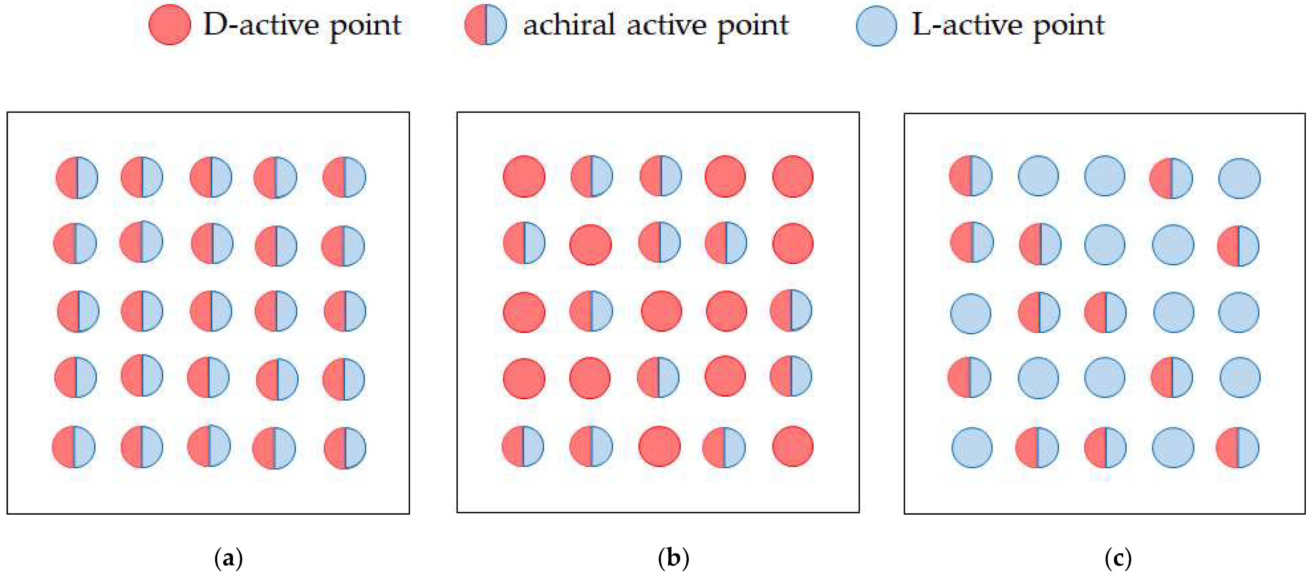
References
- Viedma, C. Chiral Symmetry Breaking During Crystallization: Complete Chiral Purity Induced by Nonlinear Autocatalysis and Recycling. Phys. Rev. Lett. 2005, 94, 065504. [Google Scholar] [CrossRef] [Scilit] [PubMed]
- Flores, J.J.; Bonner, W.A.; Massey, G.A. Asymmetric Photolysis of (RS)-Leucine with Circularly Polarized Ultraviolet Light. J. Am. Chem. Soc. 1977, 99, 3622–3625. [Google Scholar] [CrossRef] [Scilit] [PubMed]
- Rikken, G.L.J.A.; Raupach, E. Enantioselective Magnetochiral Photochemistry. Nature 2000, 405, 932–935. [Google Scholar] [CrossRef] [Scilit] [PubMed]
- Noorduim, W.L.; Bode, A.A.C.; van der Meijden, M.; Meekes, H.; van Etteger, A.F.; van Enckevort, W.J.P.; Christianen, P.C.M.; Kaptein, B.; Kellogg, R.M.; Rasing, T.; et al. Complete Chiral Symmetry Breaking of an Amino Acid Derivative Directed by Circularly Polarized Light. Nat. Chem. 2009, 1, 729–732. [Google Scholar] [CrossRef] [Scilit]
- Micali, M.; Engelkamp, H.; van Rhee, P.G.; Christianen, P.C.M.; Scolaro, L.M.; Maan, J.C. Selection of Supramolecular Chirality by Application of Rotational and Magnetic Forces. Nat. Chem. 2012, 4, 201–207. [Google Scholar] [CrossRef] [Scilit]
- Kondepudi, D.K.; Kaufman, R.J.; Singh, N. Chiral Symmetry Breaking in Sodium Chloride Crystallization. Science 1990, 250, 975–976. [Google Scholar] [CrossRef] [Scilit]
- Ribó, J.M.; Crusats, J.; Sagués, F.; Claret, J.; Rubires, R. Chiral Sign Induction by Vortices During the Formation of Mesophases in Stirred Solutions. Science 2001, 292, 2063–2066. [Google Scholar] [CrossRef] [Scilit]
- Tsujimoto, Y.; Ie, M.; Ando, Y.; Yamamoto, T.; Tsuda, A. Spectroscopic Visualization of Right- and Left-Handed Helical Alignments of DNA in Chiral Vortex Flows. Bull. Chem. Soc. Jpn. 2011, 84, 1031–1038. [Google Scholar] [CrossRef] [Scilit]
- Bolm, C.; Bienewald, F.; Seger, A. Asymmetric Autocatalysis with Amplification of Chirality. Angew. Chem. Int. Ed. Engl. 1996, 35, 1657–1659. [Google Scholar] [CrossRef] [Scilit]
- Uwaha, M. A Model for Complete Chiral Crystallization. J. Phys. Soc. Jpn. 2004, 73, 2601–2603. [Google Scholar] [CrossRef] [Scilit]
- Bargueño, P. Chirality and Gravitational Parity Violation. Chirality 2015, 27, 375–381. [Google Scholar] [CrossRef] [Scilit] [PubMed]
- Avalos, M.; Babiano, R.; Cintas, P.; Jiménes, J.L.; Palacios, J.C.; Barron, L.D. Absolute Asymmetric Synthesis under Physical Fields: Facts and Fictions. Chem. Rev. 1998, 98, 2391–2404. [Google Scholar] [CrossRef] [Scilit] [PubMed]
- Wächtershäuser, G. Before Enzymes and Templates: Theory of Surface Metabolism. Microbiol. Rev. 1988, 52, 452–484. [Google Scholar] [CrossRef] [PubMed]
- Yamamoto, M.; Nakamura, R.; Kasaya, T.; Kumagai, H.; Suzuki, K.; Takai, K. Spontaneous and Widespread Electricity Generation in Natural Deep-Sea Hydrothermal Fields. Angew. Chem. Int. Ed. 2017, 56, 5725–5728. [Google Scholar] [CrossRef] [Scilit]
- Burton, W.K.; Cabrera, N.; Frank, F.C. Role of Dislocations in Crystal Growth. Nature 1949, 163, 398–399. [Google Scholar] [CrossRef] [Scilit]
- Burton, W.K.; Cabrera, N.; Frank, F.C. The Growth of Crystals and the Equilibrium Structure of their Surfaces. Philos. Trans. R. Soc. Lond. Ser. A Math. Phys. Sci. 1951, 243, 299–358. [Google Scholar] [CrossRef] [Scilit]
- Yanson, Y.I.; Rost, M.J. Structural Accelerating Effect of Chloride on Copper Electrodeposition. Angew. Chem. Int. Ed. 2013, 52, 2454–2458. [Google Scholar] [CrossRef] [Scilit]
- Morimoto, R.; Miura, M.; Sugiyama, A.; Miura, M.; Oshikiri, Y.; Mogi, I.; Yamauchi, Y.; Takagi, S.; Aogaki, R. Theory of Chiral Electrodeposition by Chiral Micro-Nano-Vortices under a Vertical Magnetic Field -1: 2D Nucleation by Micro-Vortices. Magnetochemistry 2022, 8, 71. [Google Scholar] [CrossRef] [Scilit]
- Morimoto, R.; Miura, M.; Sugiyama, A.; Miura, M.; Oshikiri, Y.; Mogi, I.; Yamauchi, Y.; Aogaki, R. Theory of Chiral Electrodeposition by Micro-Nano-Vortexes under a Vertical Magnetic Field-2: Chiral Three-Dimensional (3D) Nucleation by Nano-Vortexes. Magnetochemistry 2024, 10, 25. [Google Scholar] [CrossRef] [Scilit]
- Rikken, G.L.J.A.; Fölling, J.; Wyder, P. Electrical Magnetochiral Anisotropy. Phys. Rev. Lett. 2001, 87, 236602. [Google Scholar] [CrossRef] [Scilit]
- Mogi, I.; Aogaki, R.; Takahashi, K. Chiral symmetry breaking in magnetoelectrochemical etching with chloride additives. Molecules 2018, 23, 19. [Google Scholar] [CrossRef] [Scilit]
- Takagi, S.; Asada, T.; Oshikiri, Y.; Miura, M.; Morimoto, R.; Sugiyama, A.; Mogi, I.; Aogaki, R. Nanobubble formation from ionic vacancies in an electrode reaction on a fringed electrode under a uniform vertical magnetic field—1. Formation process in a vertical magnetohydrodynamic (MHD) flow. J. Electroanal. Chem. 2022, 914, 116291. [Google Scholar] [CrossRef] [Scilit]
- Takagi, S.; Asada, T.; Oshikiri, Y.; Miura, M.; Morimoto, R.; Sugiyama, A.; Mogi, I.; Aogaki, R. Nanobubble formation from ionic vacancies in an electrode reaction on a fringed electrode under a uniform vertical magnetic field—2. Measurement of the angular velocity of a vertical magnetohydrodynamic (MHD) flow by the microbubbles originating from ionic vacancies. J. Electroanal. Chem. 2022, 916, 116375. [Google Scholar] [CrossRef] [Scilit]
- Aogaki, R. Theory of stable formation of ionic vacancy in a liquid solution. Electrochemistry 2008, 76, 458–465. [Google Scholar] [CrossRef] [Scilit]
- Aogaki, R.; Sugiyama, A.; Miura, M.; Oshikiri, Y.; Miura, M.; Morimoto, R.; Takagi, S.; Mogi, I.; Yamauchi, Y. Origin of nanobubbles electrochemically formed in a magnetic field: Ionic vacancy production in electrode reaction. Sci. Rep. 2016, 6, 28297. [Google Scholar] [CrossRef] [Scilit]
- Aogaki, R.; Motomura, K.; Sugiyama, A.; Morimoto, R.; Mogi, I.; Miura, M.; Asanuma, M.; Oshikiri, Y. Measurement of the lifetime of ionic vacancy by the cyclotron-MHD electrode. Magnetohydrodynamics 2012, 48, 289–297. [Google Scholar] [CrossRef] [Scilit]
- Sugiyama, A.; Morimoto, R.; Osaka, T.; Mogi, I.; Asanuma, M.; Miura, M.; Oshikiri, Y.; Yamauchi, Y.; Aogaki, R. Lifetime of ionic vacancy created in redox electrode reaction measured by cyclotron MHD electrode. Sci. Rep. 2016, 6, 19795. [Google Scholar] [CrossRef] [Scilit]
- Mogi, I.; Morimoto, R.; Aogaki, R.; Takahashi, K. Surface chirality in rotational magnetoelectrodeposition of copper films. Magnetochemistry 2019, 5, 53–60. [Google Scholar] [CrossRef] [Scilit]
- Mogi, I.; Morimoto, R.; Aogaki, R.; Watanabe, K. Surface chirality induced by rotational electrodeposition in magnetic fields. Sci. Rep. 2013, 3, 2574. [Google Scholar] [CrossRef] [Scilit]
- Mogi, I.; Morimoto, R.; Aogaki, R.; Takahashi, K. Effects of vertical MHD flows and cell rotation on surface chirality in magnetoelectrodeposition. IOP Conf. Ser. Mater. Sci. Eng. 2018, 424, 012024. [Google Scholar] [CrossRef] [Scilit]
- Chandrasekhar, S. Hydrodynamic and Hydromagnetic Stability; Oxford University Press: London, UK, 1961; pp. 87–148. [Google Scholar]
- Mogi, I.; Aogaki, R.; Takahashi, K. Fluctuation effects of magnetohydrodynamic micro-vortices on odd chirality in magnetoelectrolysis. Magnetochemistry 2020, 6, 43–51. [Google Scholar] [CrossRef] [Scilit]
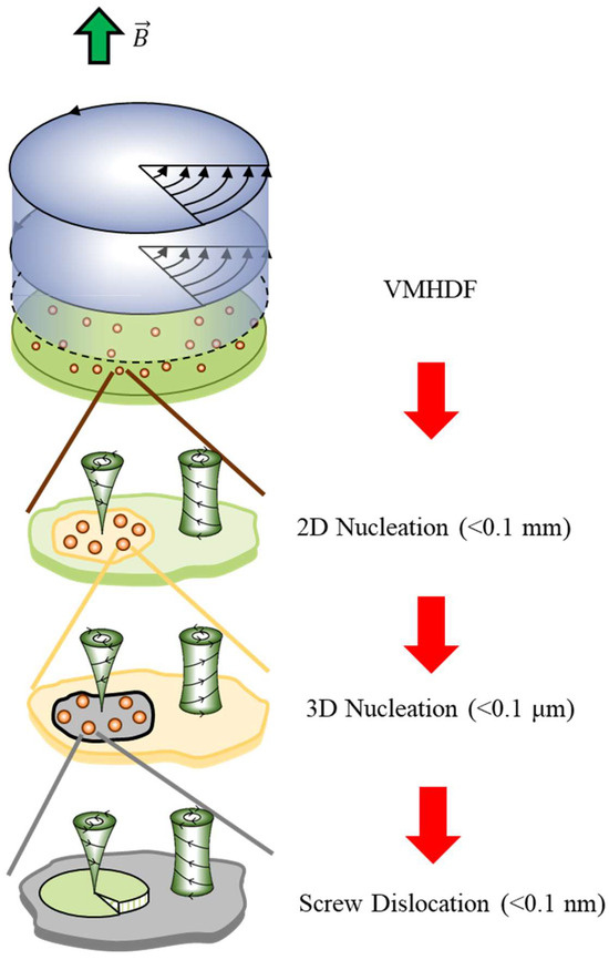
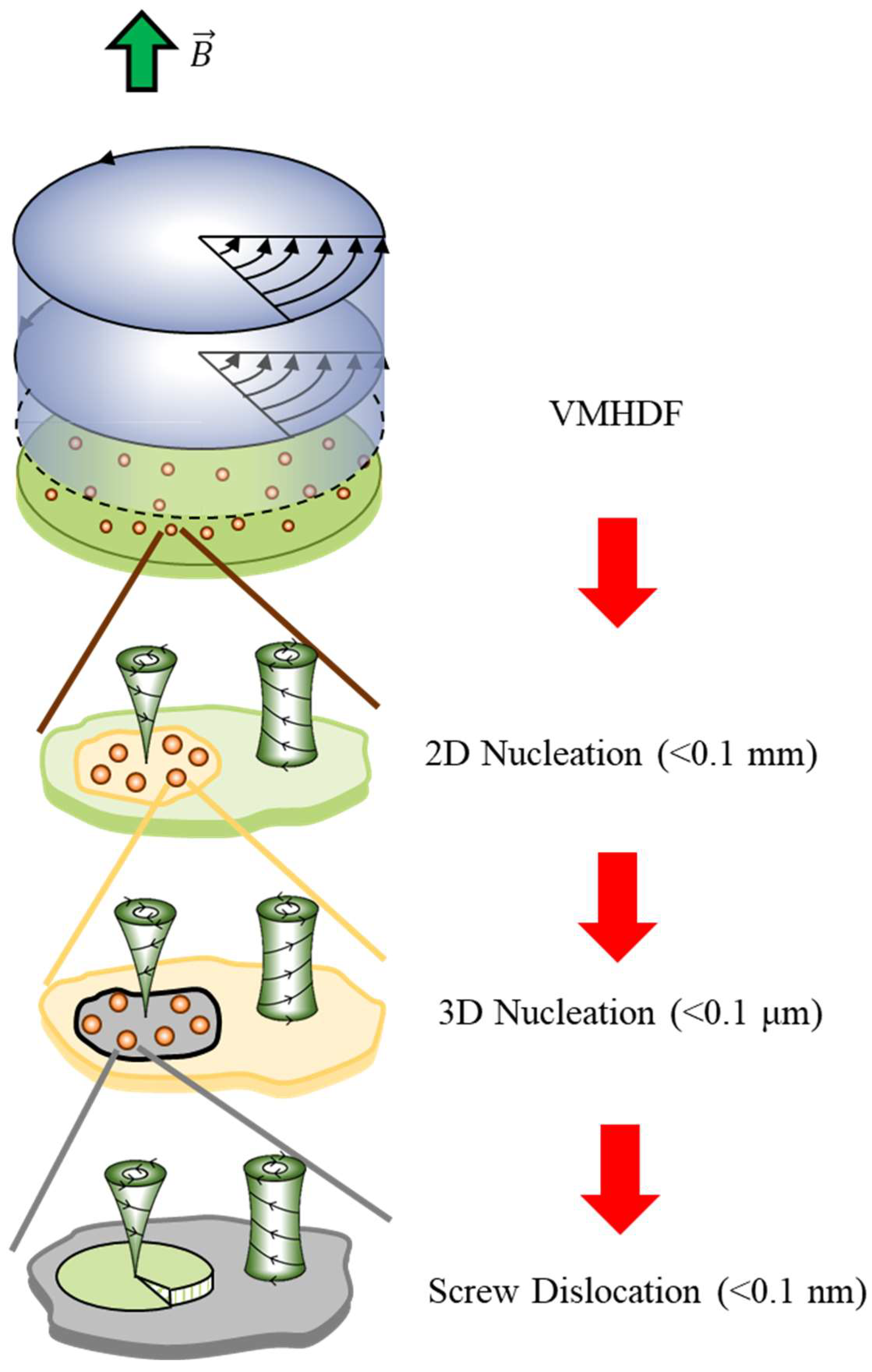
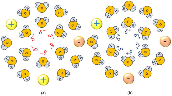
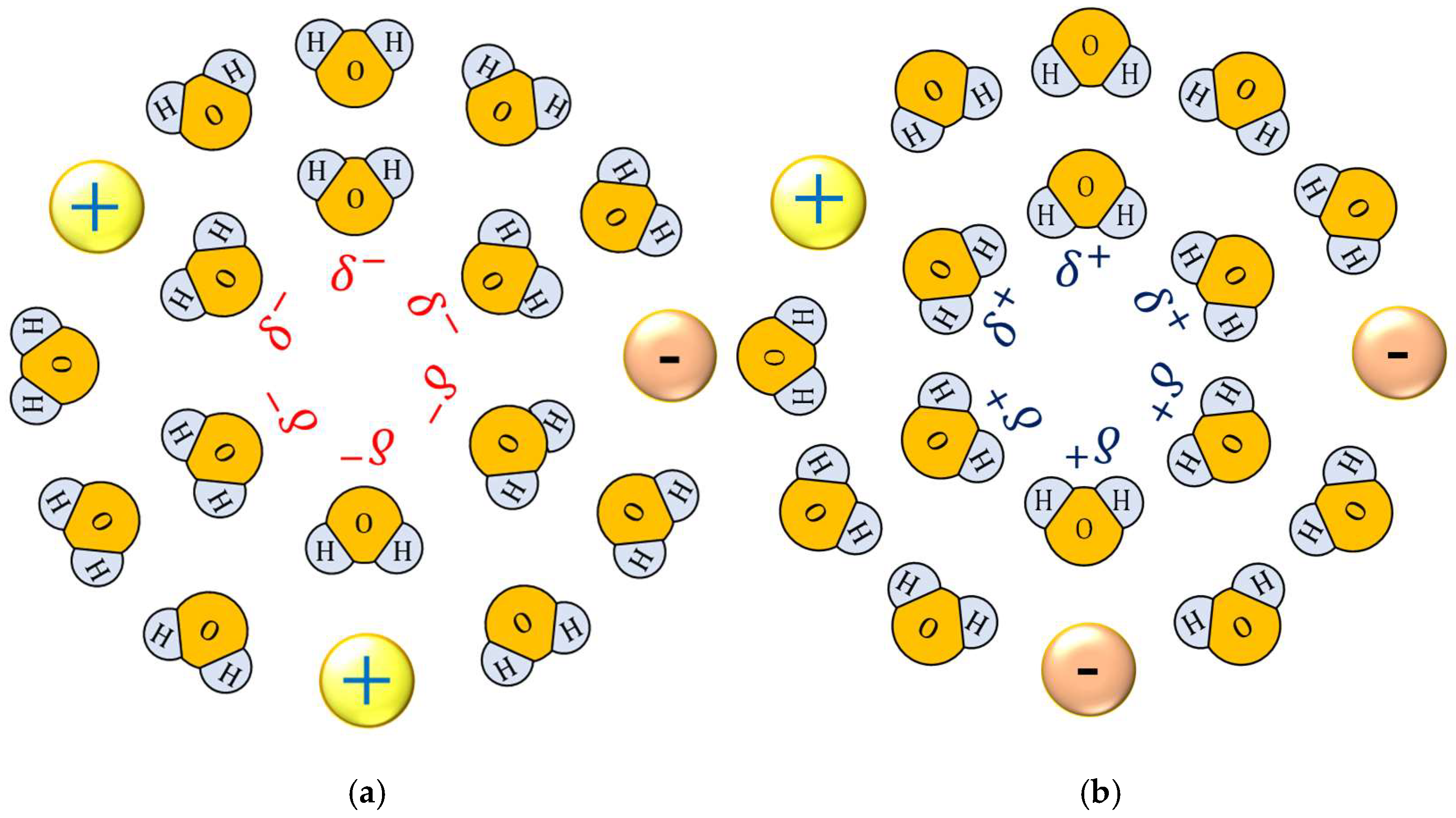
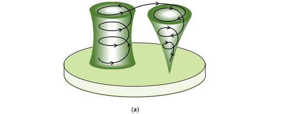
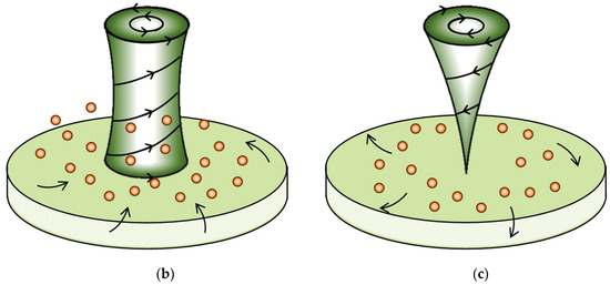
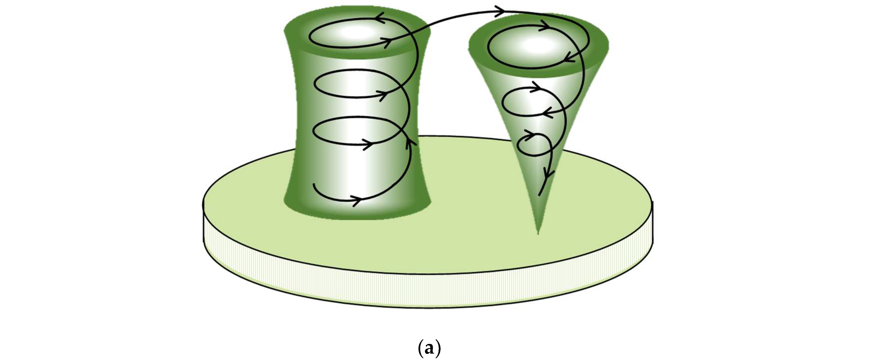
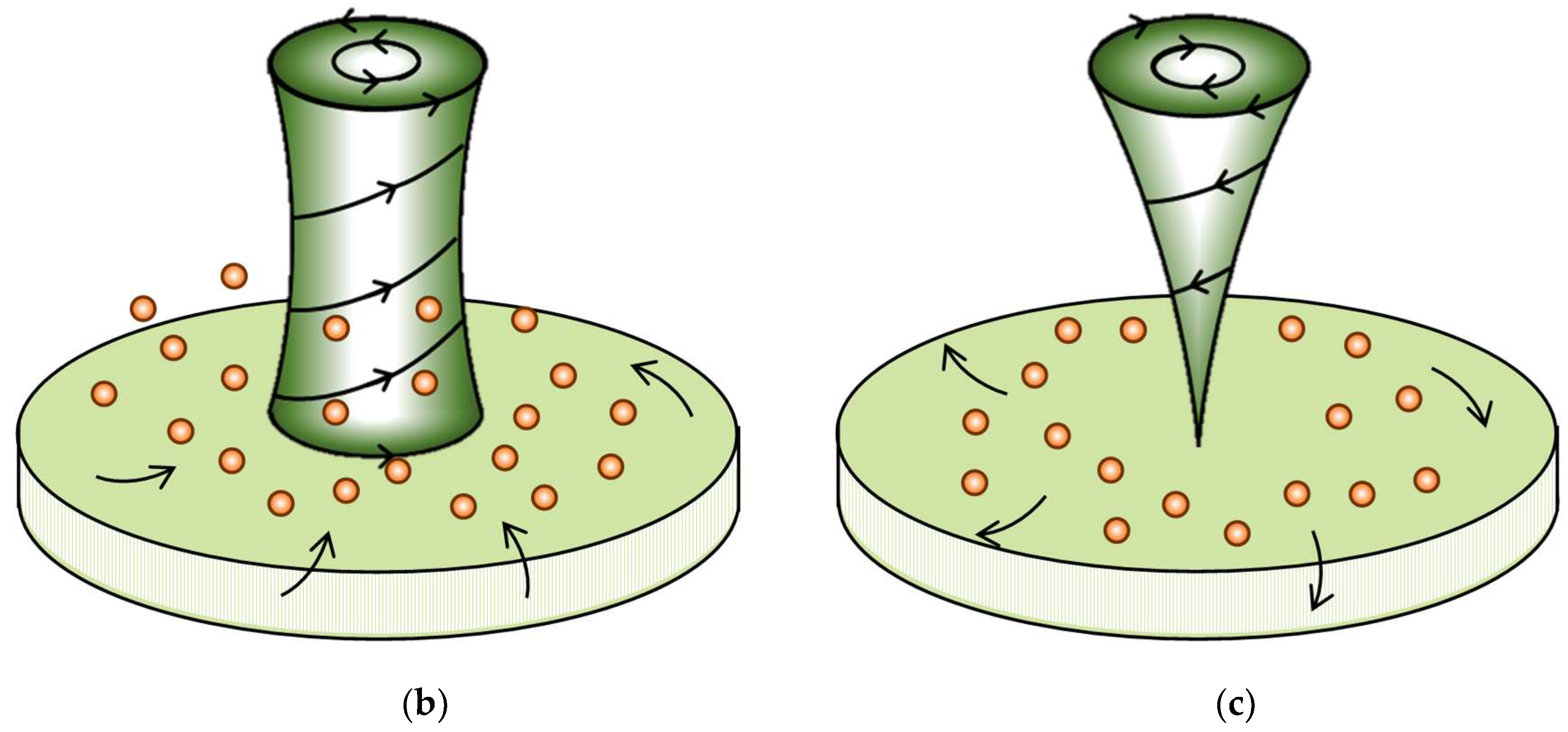
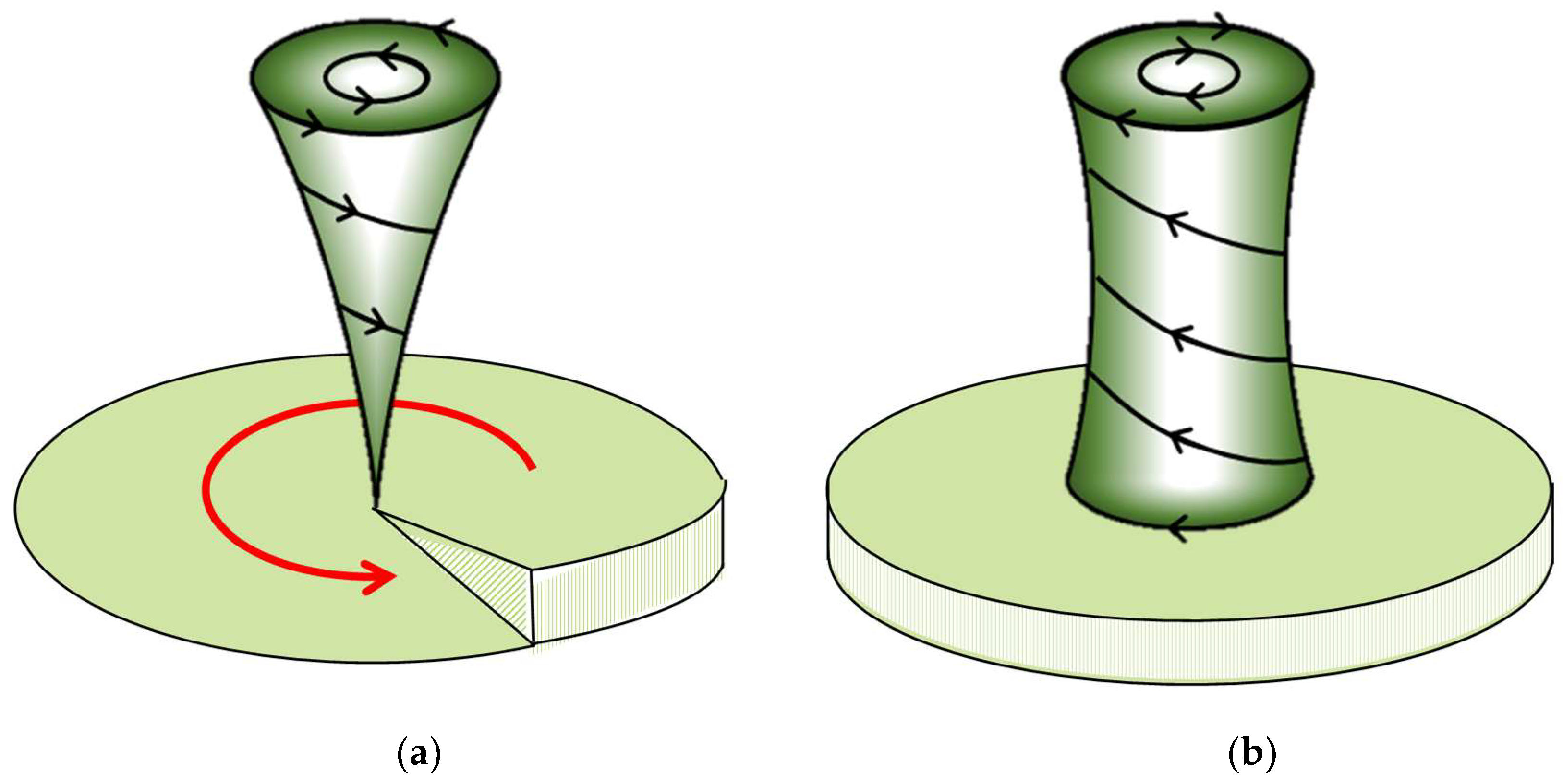
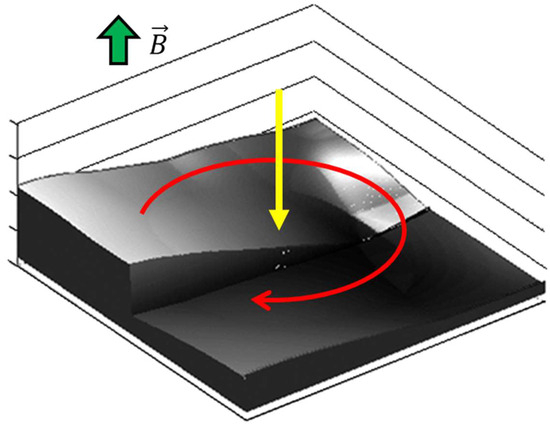
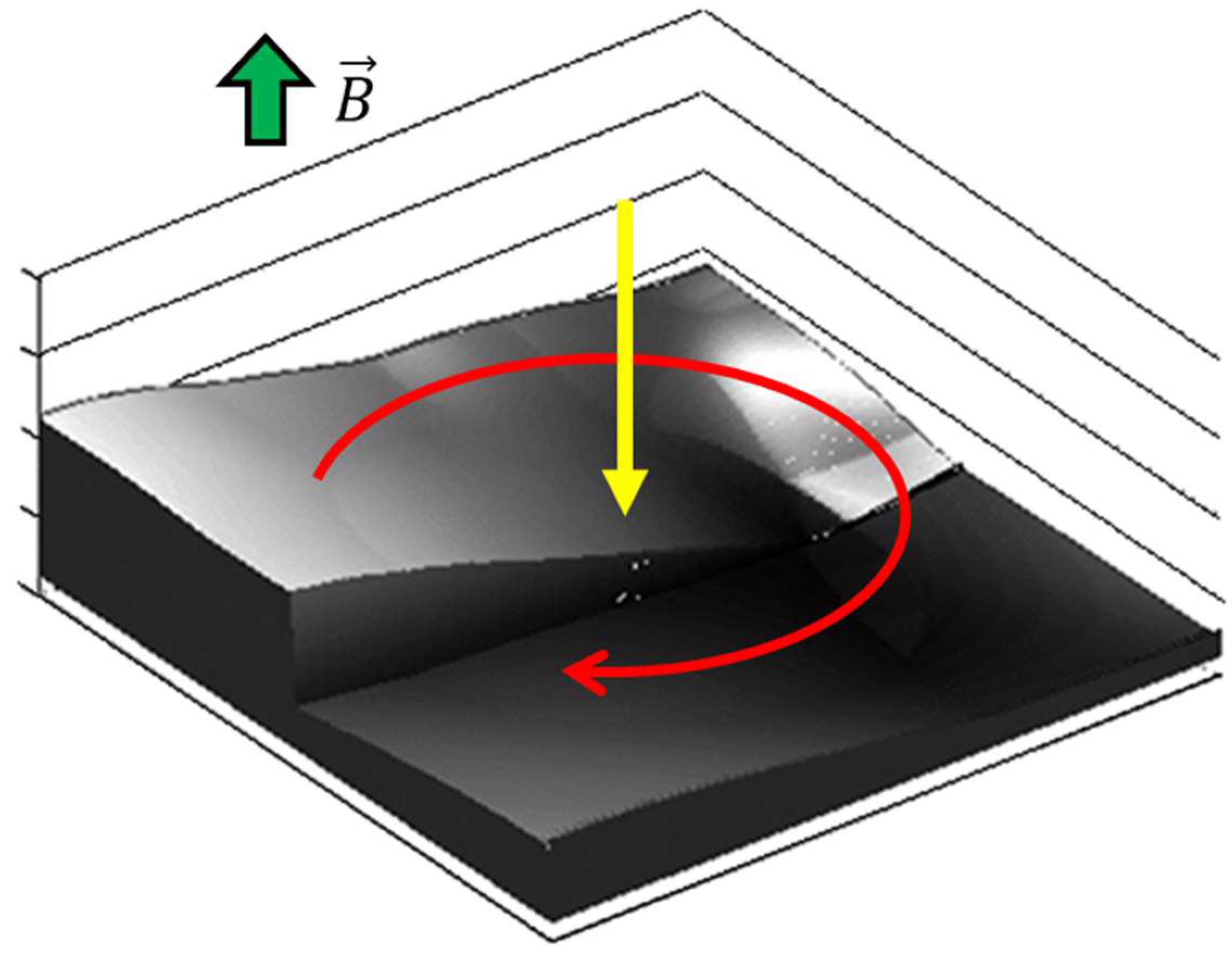
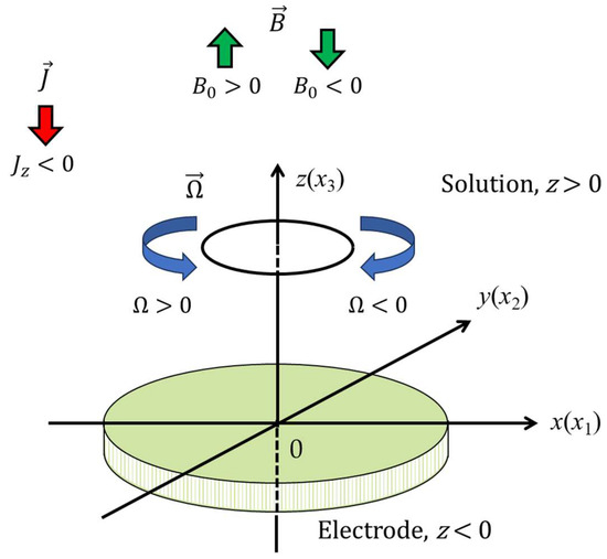
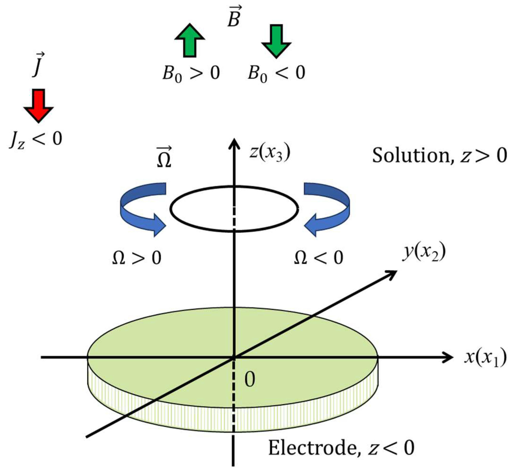
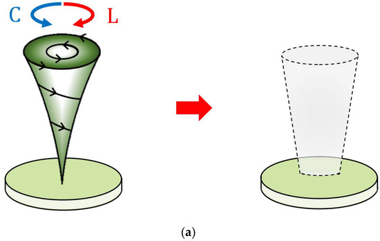
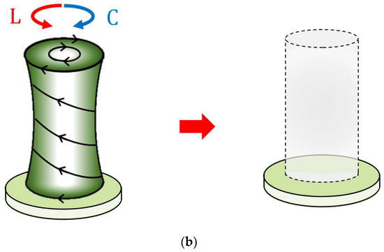
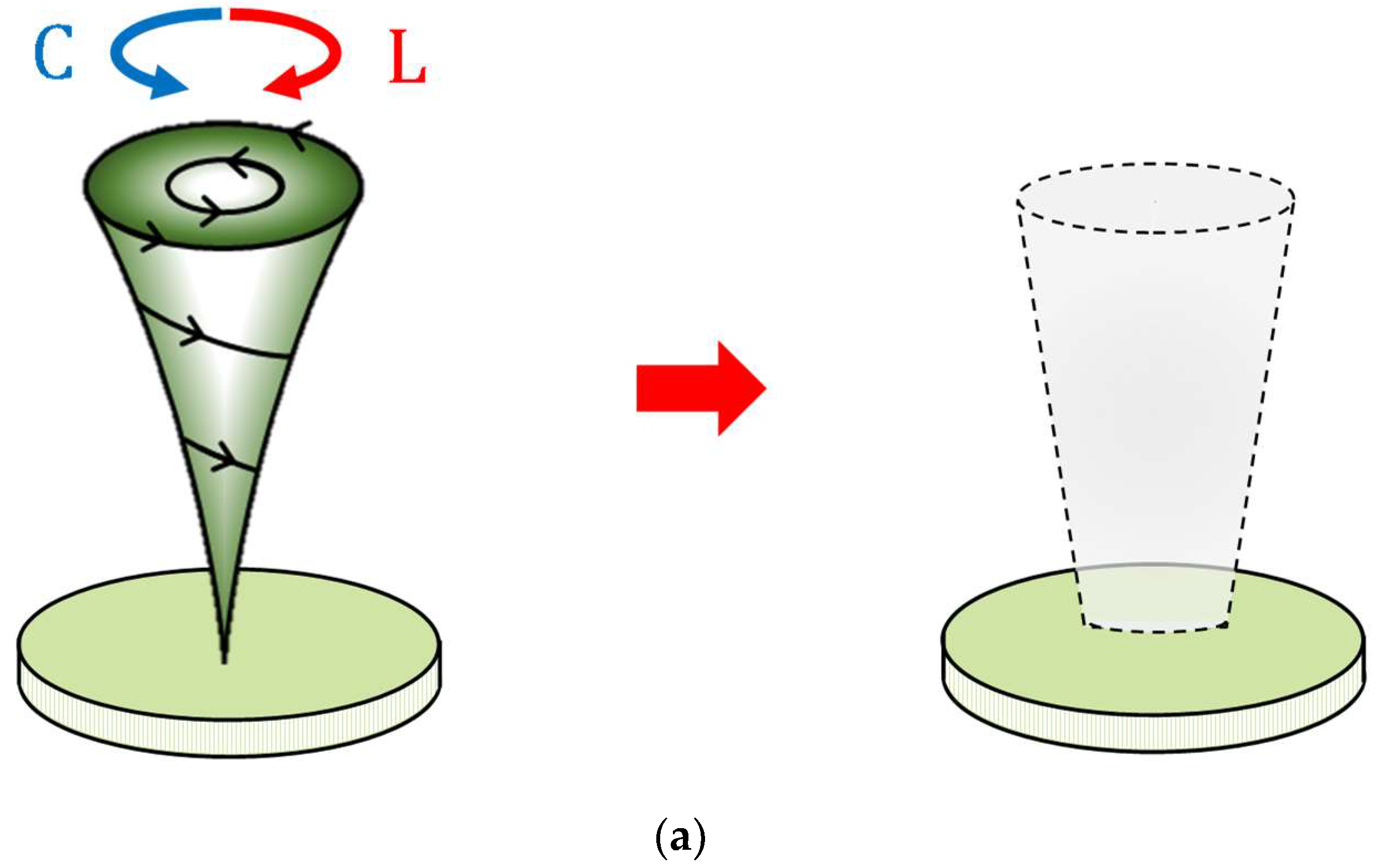
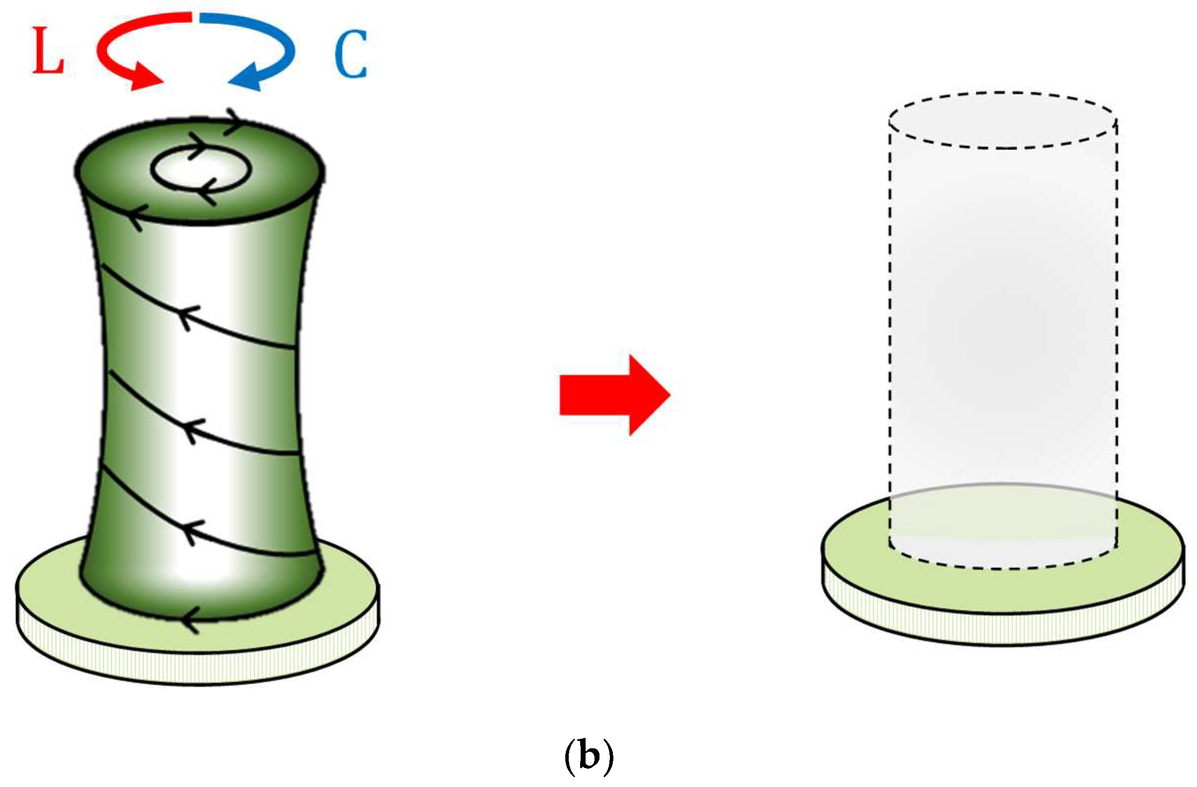
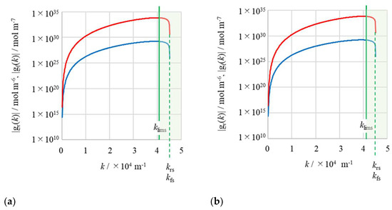
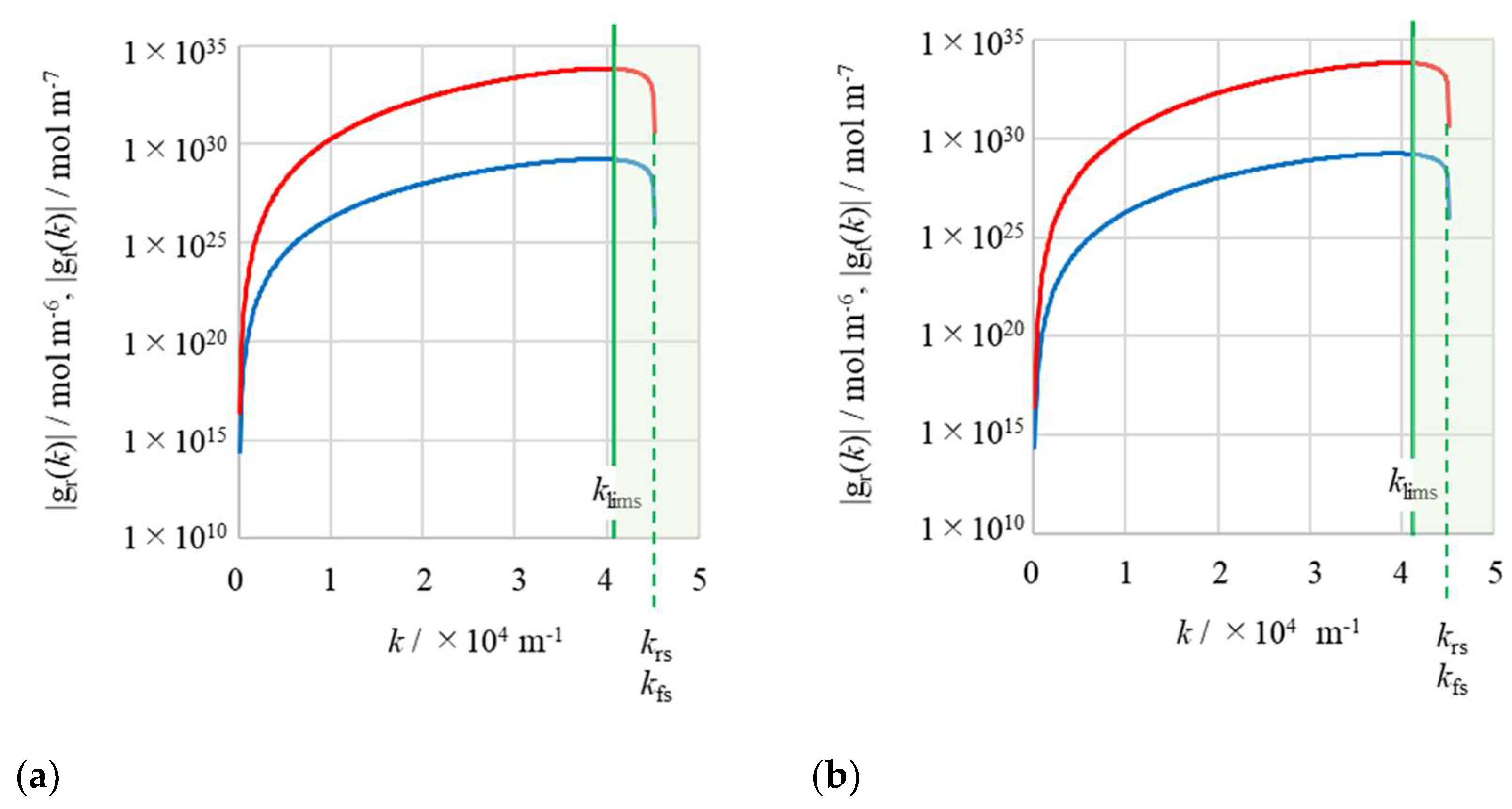
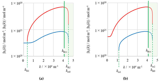
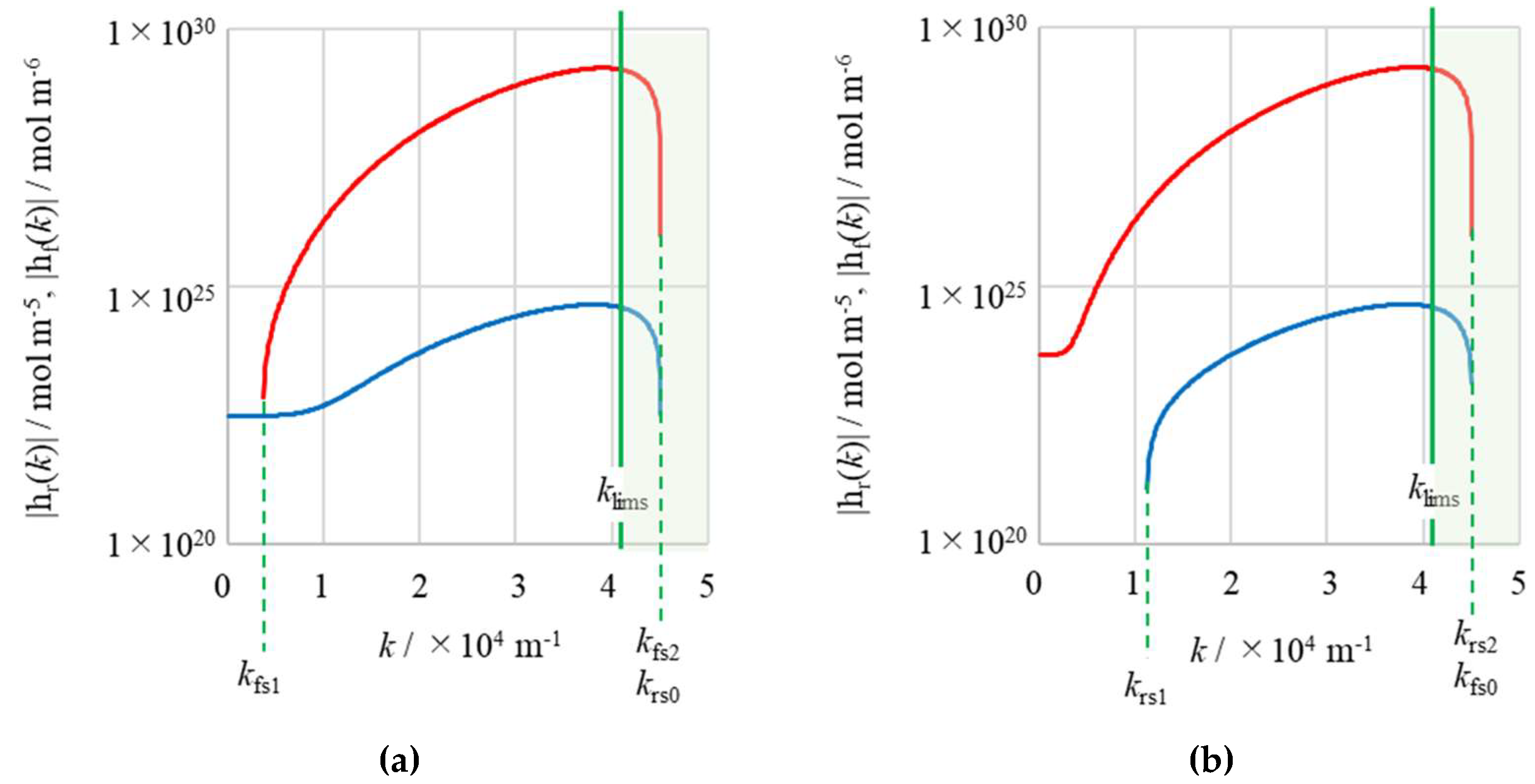
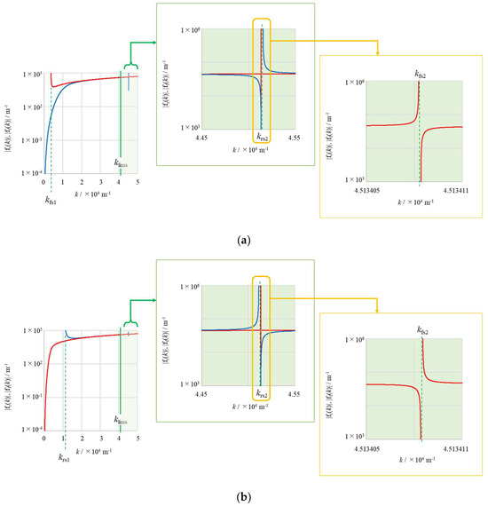
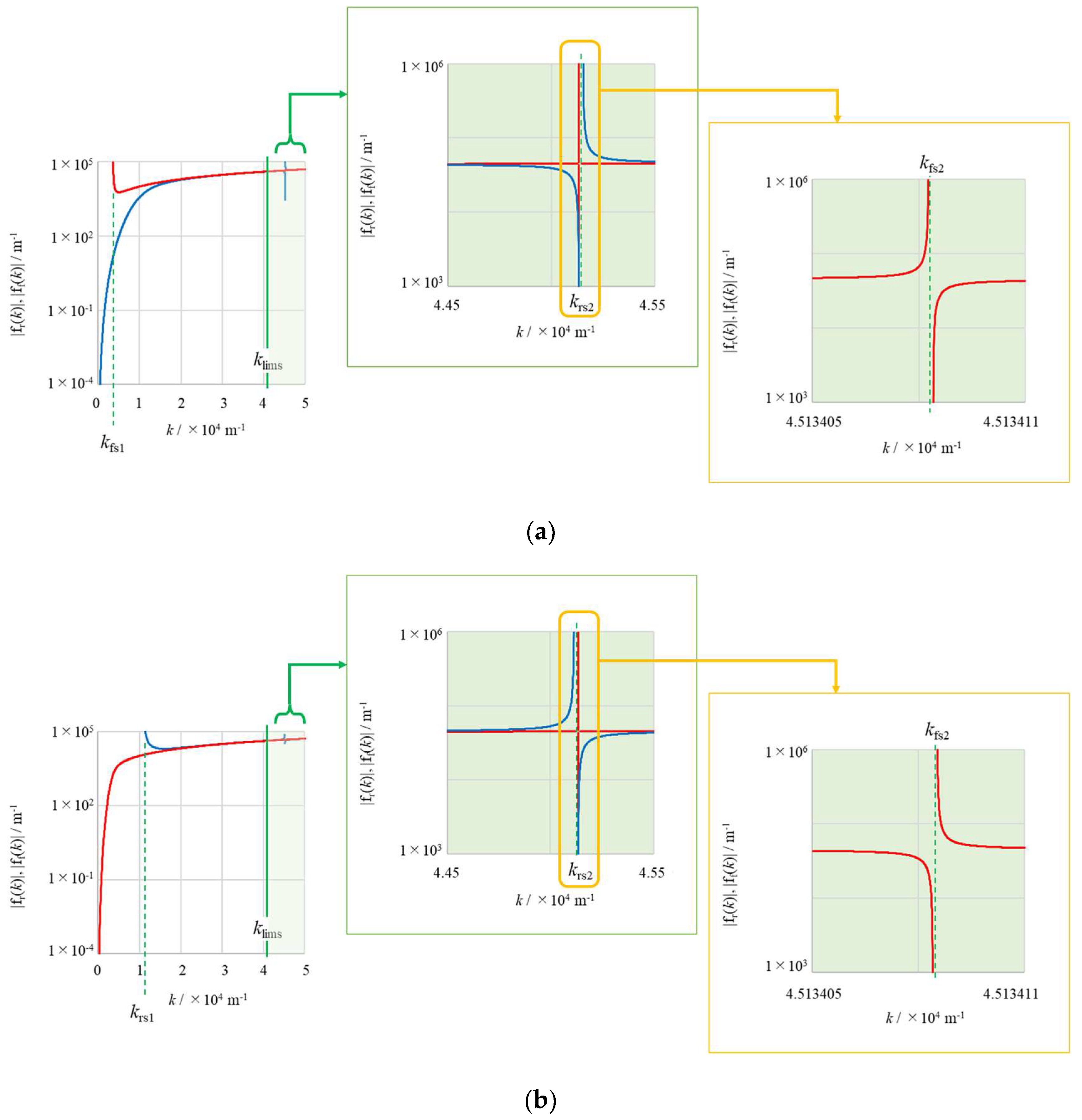
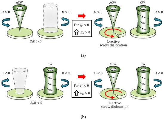
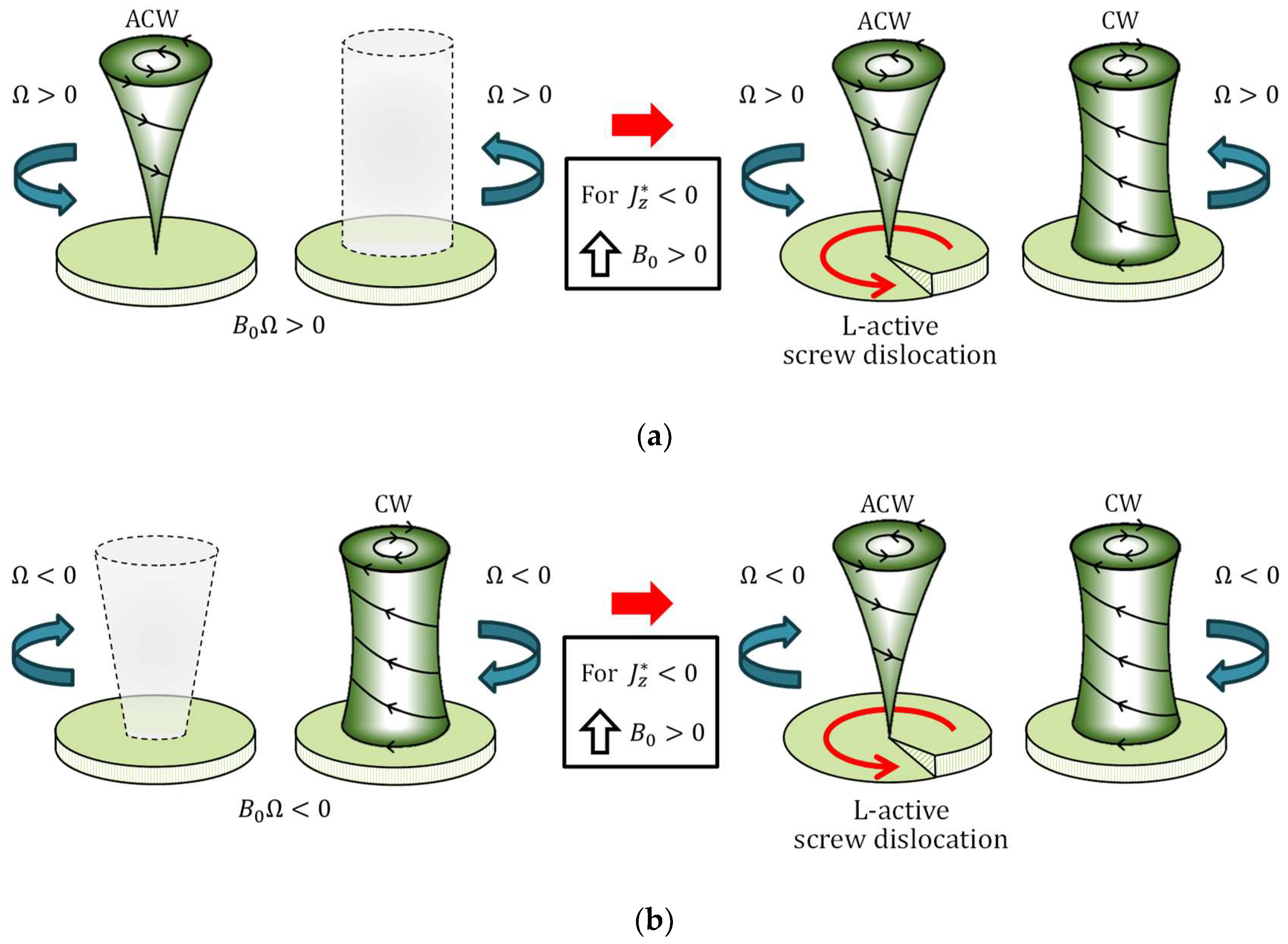
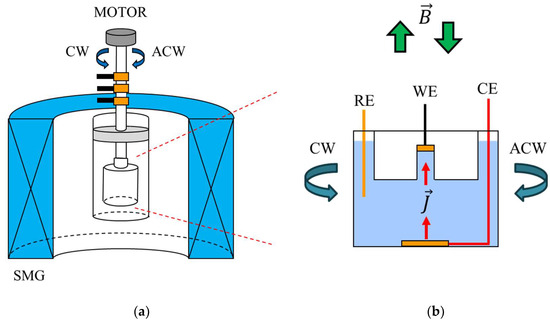
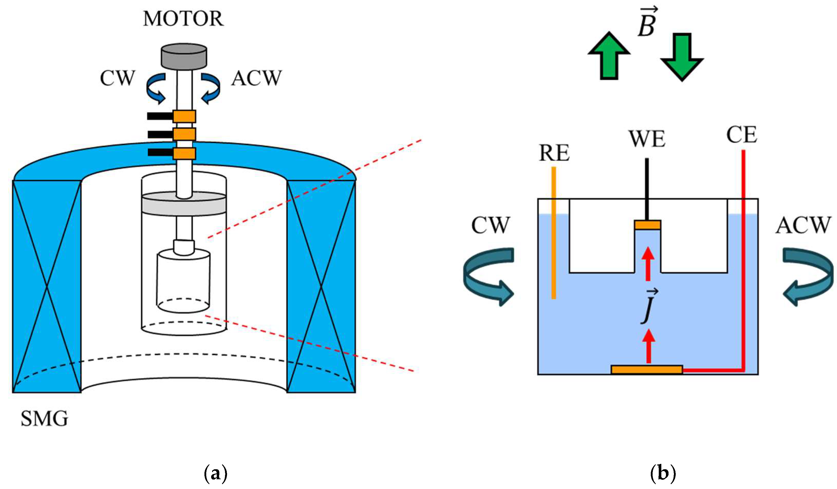
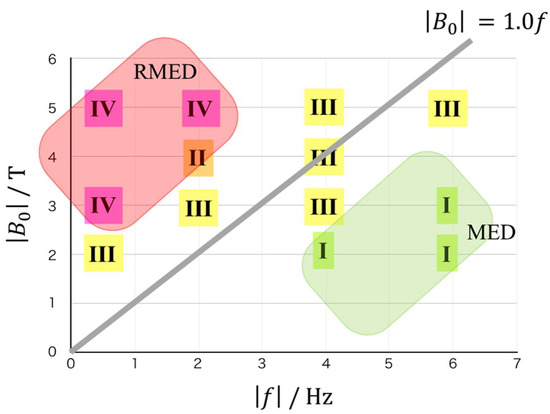
Disclaimer/Publisher’s Note: The statements, opinions and data contained in all publications are solely those of the individual author(s) and contributor(s) and not of MDPI and/or the editor(s). MDPI and/or the editor(s) disclaim responsibility for any injury to people or property resulting from any ideas, methods, instructions or products referred to in the content. |
© 2025 by the authors. Licensee MDPI, Basel, Switzerland. This article is an open access article distributed under the terms and conditions of the Creative Commons Attribution (CC BY) license (https://creativecommons.org/licenses/by/4.0/).