Abstract
In the current paper, an analysis of magnetohydrodynamic Williamson nanofluid boundary layer flow is presented, with multiple slips in a porous medium, using a newly designed human-brain-inspired Ricker wavelet neural network solver. The solver employs a hybrid approach that combines genetic algorithms, serving as a global search method, with sequential quadratic programming, which functions as a local optimization technique. The heat and mass transportation effects are examined through a stretchable surface with radiation, thermal, and velocity slip effects. The primary flow equations, originally expressed as partial differential equations (PDEs), are changed into a dimensionless nonlinear system of ordinary differential equations (ODEs) via similarity transformations. These ODEs are then numerically solved with the proposed computational approach. The current study has significant applications in a variety of practical engineering and industrial scenarios, including thermal energy systems, biomedical cooling devices, and enhanced oil recovery techniques, where the control and optimization of heat and mass transport in complex fluid environments are essential. The numerical outcomes gathered through the designed scheme are compared with reference results acquired through Adam’s numerical method in terms of graphs and tables of absolute errors. The rapid convergence, effectiveness, and stability of the suggested solver are analyzed using various statistical and performance operators.
1. Introduction
For the last few decades, nanofluids have extensively been used in the medical, biological, and engineering fields due to their distinctive characteristics, including optimal wetting, magnetic, thermal, and electrical properties that boost their performance. Nanoparticles are nanometer-sized, tiny particles based on metals, oxides, and carbides that generate nanofluids when mixed with fluids like oil, ethylene, or water. Nanofluids are highly beneficial for the enhancement in thermal conductivity in Newtonian and non-Newtonian fluids. Research on the enhancement in thermal conductivity was first carried out in 1993 by Masuda et al. [1]. The application of nanofluids in heat and transfer phenomena with huge thermal conductivities was introduced by Choi and Eastman [2]. Nanofluids are used in diverse fields, including drug transportation [3], thermosyphon [4], biophysics [5], combustion procedures [6], refrigeration processes [7], coating processes [8], heat exchangers [9], crystal proliferation [10], and solar energy [11]. Some important results of analyzing the flow properties of different nanofluids are presented in [12,13,14,15,16,17,18,19,20].
Magnetohydrodynamics (MHDs) are defined as the passage of electrically good conducting fluids in the presence of a magnetic field. Fluid flow with the MHD effect has been studied by a large number of researchers because of its practical applicability in the areas of cosmic fluid dynamics, polymer industry, agriculture, solar physics, astrophysics, polymer industry, metallurgy, and geophysics. Recently, the MHD phenomenon with heat and mass transfer impacts along an extended porous surface has been examined by different scientists. Shamshuddin et al. [21] examined microorganism nanofluidic flow with an induced heat source along a stretchable surface (SAS) through porous media. Khan et al. [22] investigated heat transfer impact in the case of MHD thin-film flow over a SAS. Alriheli et al. [23] discussed a dissipative MHD nanofluidic flow over a SAS through a porous medium with a chemical reaction effect. Srivastava et al. [24] discussed MHD boundary-layer (BL) flow across a SAS using different slips in a porous medium. Biswal et al. [25] studied the MHD stagnation point flow through a SAS embedded in a porous medium in terms of heat and mass transfer effects. Sitamahalakshmi et al. [26] examined MHD Casson fluidic flow through a SAS in the shape of a permeable vessel with heat and mass transfer impacts.
Non-Newtonian fluid models have several engineering and industrial-type applications, including photographic films, glass blowing, polymer-coated sheets, and cosmetic items. The rheological characteristics of various fluids are not possible to explain using only Navier–Stokes equations. To fill this gap, various rheological paradigms have been developed, including the Jeffery model, the power-law model, the Cross model, and the Williamson model. Williamson [27] proposed a model that briefly explains the flow of pseudoplastic fluids. Many researchers have used this model because it tends to show the viscoelastic characteristics of materials. Jabeen et al. [28] numerically investigated Williamson nanofluid (WNF) BL flow under the effects of activation energy and dissipation using the bvp4c technique. Dyapa et al. [29] discussed MHD-WNF flow with Dufour/Soret effects using the Keller–Box technique. Dulal Pal et al. [30] examined double diffusive MHD-WNF flow for entropy generation with thermal radiation impact using the spectral quasi-linearization technique. Nayak et al. [31] analyzed MHD-WNF flow with fuzzy parametric behavior using the Runge–Kutta fourth-order technique. Kairi et al. [32] determined bioconvective flow using WNF and the Runge–Kutta–Fehlberg method and concluded that the larger value of the Williamson parameter diminishes the heat and mass transfer effects. Ahmed et al. [33] studied radiative nonlinear WNF flow through a wavy cone using the implicit finite differences method and concluded that nanofluidic flow decreases with an escalation in the value of the Williamson number. Patil et al. [34] investigated WNF flow over a vertical cone using the finite difference technique as well as the quasi-linearization method.
The human-brain-inspired (HBI) Ricker wavelet neural network (RWNN) solver, i.e., the HBI-RWNN solver is a stochastic technique based on artificial neural networks (ANNs) that is constructed to handle magnetohydrodynamic Williamson nanofluid boundary-layer flow, i.e., MHD-WNF-BL flow, in terms of a nonlinear system of ODEs. ANN-based techniques have extensively been used to solve stiff nonlinear equations that are attained through the mathematical interpretation of real-world problems and are well known for their efficacy. The applications of ANN-based design techniques include the VPSA model [35], the Lassa fever model [36], the Falkner–Skan paradigm [37], the computer virus detection model [38], the squeezing flow paradigm [39], the SEIR Ebola paradigm [40], the tuberculosis model [41], the hydrogen-based purification model [42], the corneal paradigm [43], the fluid model [44], the delay model [45], and the COVID-19 paradigms [46,47]. However, to the best of our knowledge, the HBI-RWNN technique has never been applied before to solve the MHD-WNF-BL flow model. The key features of the present research are as follows:
- A novel human-brain-inspired scheme based on Ricker wavelet neural networks was established to solve MHD Williamson nanofluid boundary-layer flow over a stretchable porous surface with multiple slip conditions.
- The MHD-WNF-BL flow problem was solved numerically to evaluate velocity, thermal gradient, and nanofluid concentration using variations in the values of the involved physical parameters based on sundry scenarios.
- Absolute errors (AEs) were evaluated through graphs and tables as a result of a comparison of the obtained numerical outcomes with reference solutions.
- The working of the HBI-RWNN solver was examined through various statistical and performance analyses.
The organization of the remaining paper is as follows: the second section demonstrates the mathematical modeling of the MHD-WNF-BL flow problem, while the third section describes the design methodology manifestation. The results with a brief discussion are presented in the fourth section, while the last section presents the conclusions as well as future work.
2. Mathematical Modeling
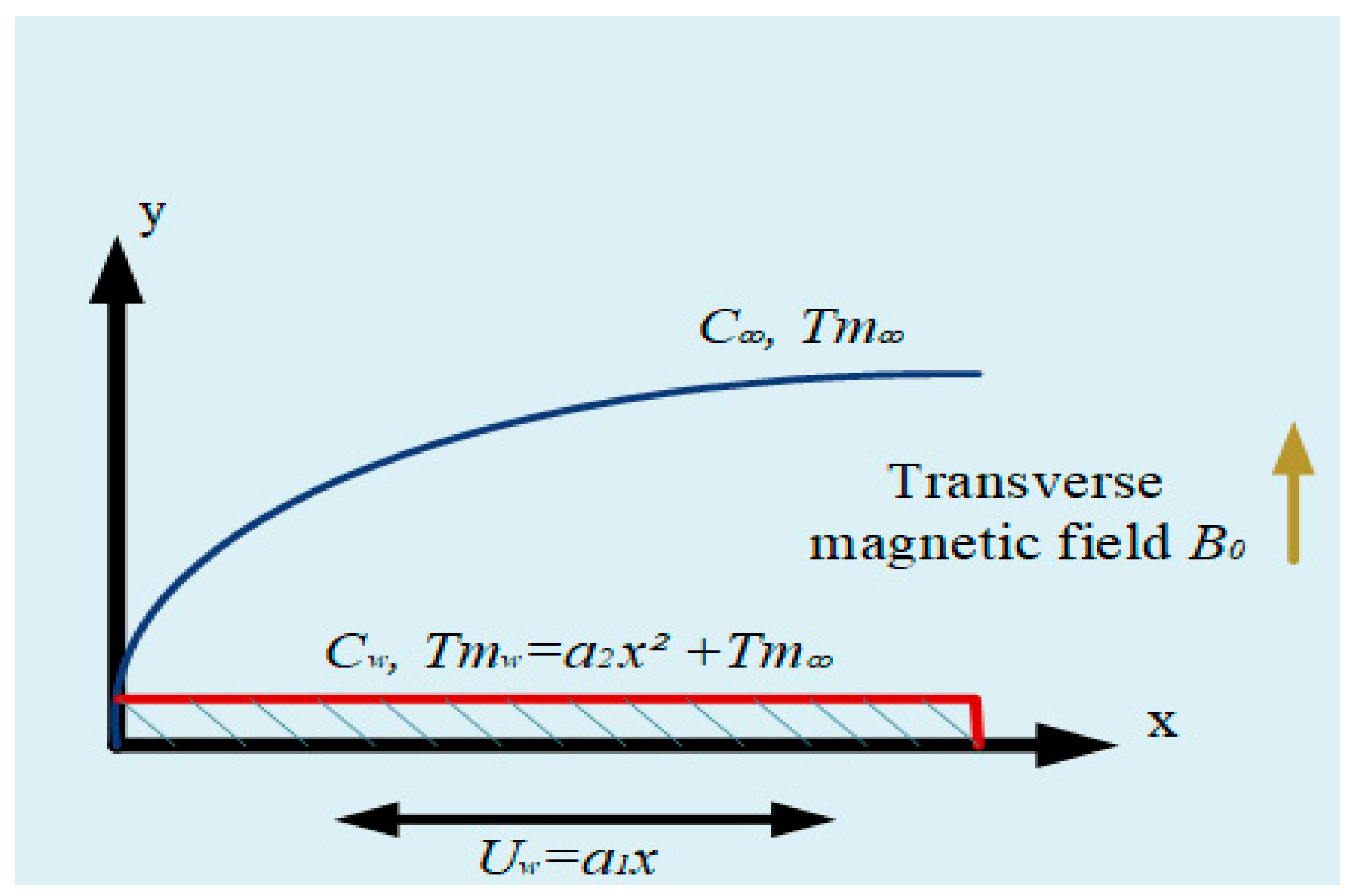
Figure 1 depicts 2-dimensional MHD-WNF-BL flow through a porous STS in x-direction expansion with velocity Uw(x) = a1x; (a1 > 0). The wall temperature is Tmw = Tm∞ + a2x2, while Cw represents the volume fraction for nanoparticles through an STS. Consistency is assumed in the shape and size of the nanoparticles, while a single-phase nanoliquid is supposed throughout the thermal equilibrium. In the presence of radiation and a magnetic field, the flow governing BL equations is [48,49,50,51]
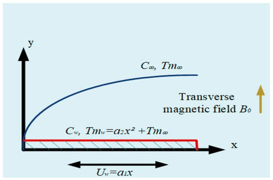
Figure 1.
MHD-WNF-BL flow model geometry.
The conditions over the boundary are
The similarity transformations employed here are
The obtained nonlinear system of ODEs is
with the following boundary conditions:
The physical parameters are formulated as
The system represented in Equations (7)–(10) is solved by assigning different values to the parameters involved in these equations, whose details are presented in Table 1.

Table 1.
Scenario-wise values assigned to the parameters in the MHD-WNF-BL flow problem.
3. Methodology
The formulation of the required numerical solution based on the HBI-RWNN solver for MHD-WNF-BL flow problem along the general form of derivatives is
The expression used in the HBI-RWNN solver is called the Ricker wavelet [52] activation function. The choice of this function was motivated by its inherent ability to capture the localized features of the solution due to their compact support and oscillatory nature, which makes it particularly effective for modeling nonlinear fluid flow dynamics with steep gradients and boundary effects. The designed solver when optimized with GA-SQP provides a robust platform for the accurate and efficient approximation of the governing differential equations. So, the obtained desired solution and highest-order derivatives have the form
The most important fitness function formulated for the MHD-WNF-BL flow problem is
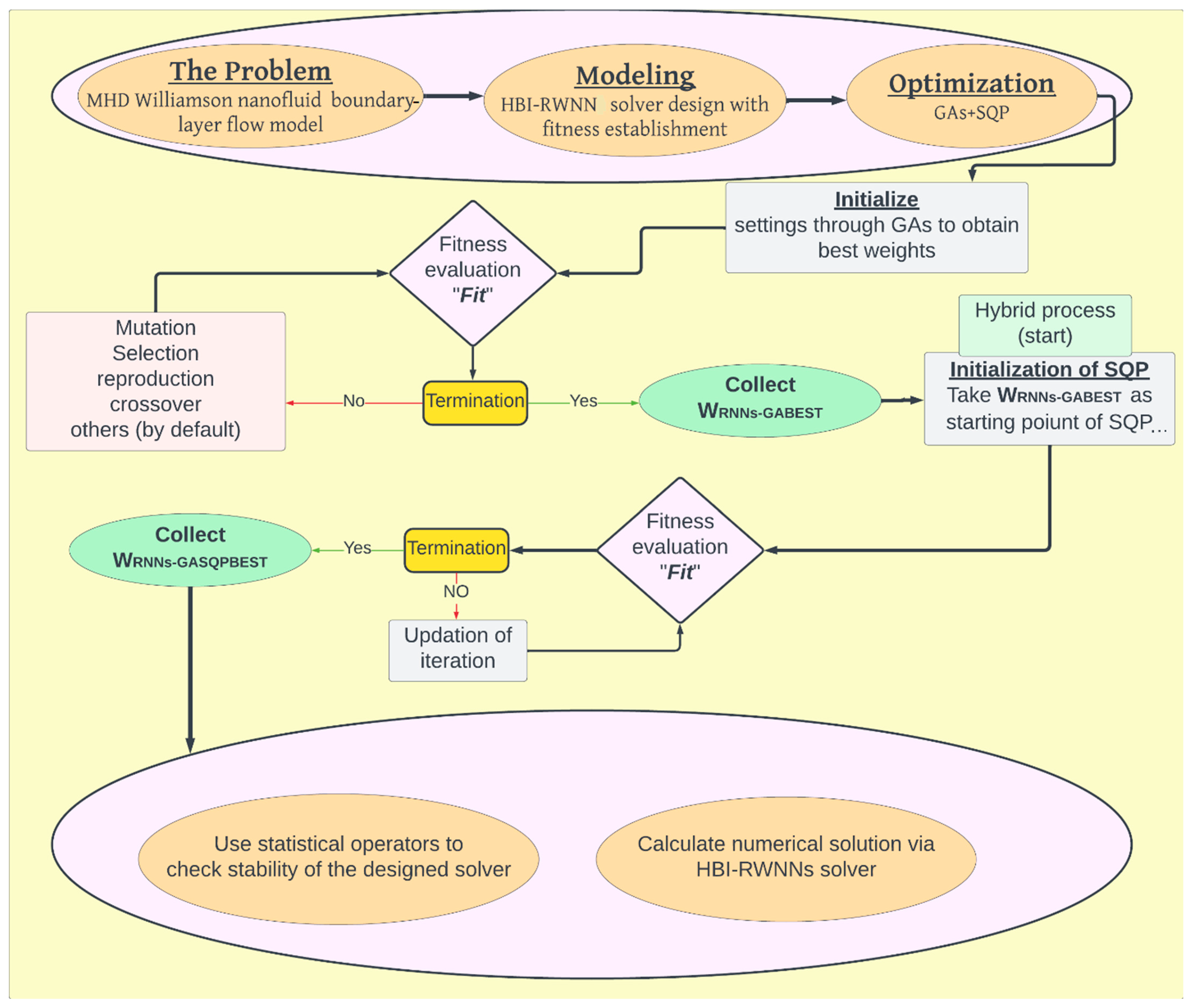
A highly accurate and desired numerical solution is generated only when Fit → 0. Figure 2 demonstrates the designed methodology’s graphical shape for solving the MHD-WNF-BL flow problem.
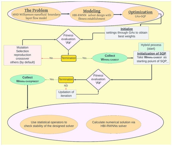
Figure 2.
Graphical abstract of HBI-RWNN algorithm for solving MHD-WNF-BL flow problem.
3.1. Learning Procedure
The optimization process to calculate the “Fit” function is accomplished by the hybrid technique, adopted using genetic algorithms (GAs) and sequential quadratic programming (SQP).
Genetic algorithms (GAs) are a strong global search scheme introduced by J. Holland [53] and are an important branch of evolutionary computation. The working of GAs depends mainly on genetics and natural selection. Some useful stochastic paradigms constructed through GAs are presented in [54,55,56,57].
Sequential quadratic programming (SQP) is one of the most powerful local search solvers [58] that can handle the nonlinearity of any order involved in real-world problems and can generate highly accurate results. Recent SQP-based applications are described in [59,60,61].
Table 2 represents the pseudo-code generated for the designed HBI-RWNN scheme to obtain numerical outcomes of the MHD-WNF-BL flow problem.
Table 2.
Pseudo-code generated for MHD-WNF-BL flow problem using HBI-RWNN solver.
3.2. Performance Metrics
To verify the reliability of the designed HBI-RWNNs solver, the results obtained through the above-formulated statistical operators for the MHD-WNF-BL flow problem should be very close to zero.
4. Results and Discussion
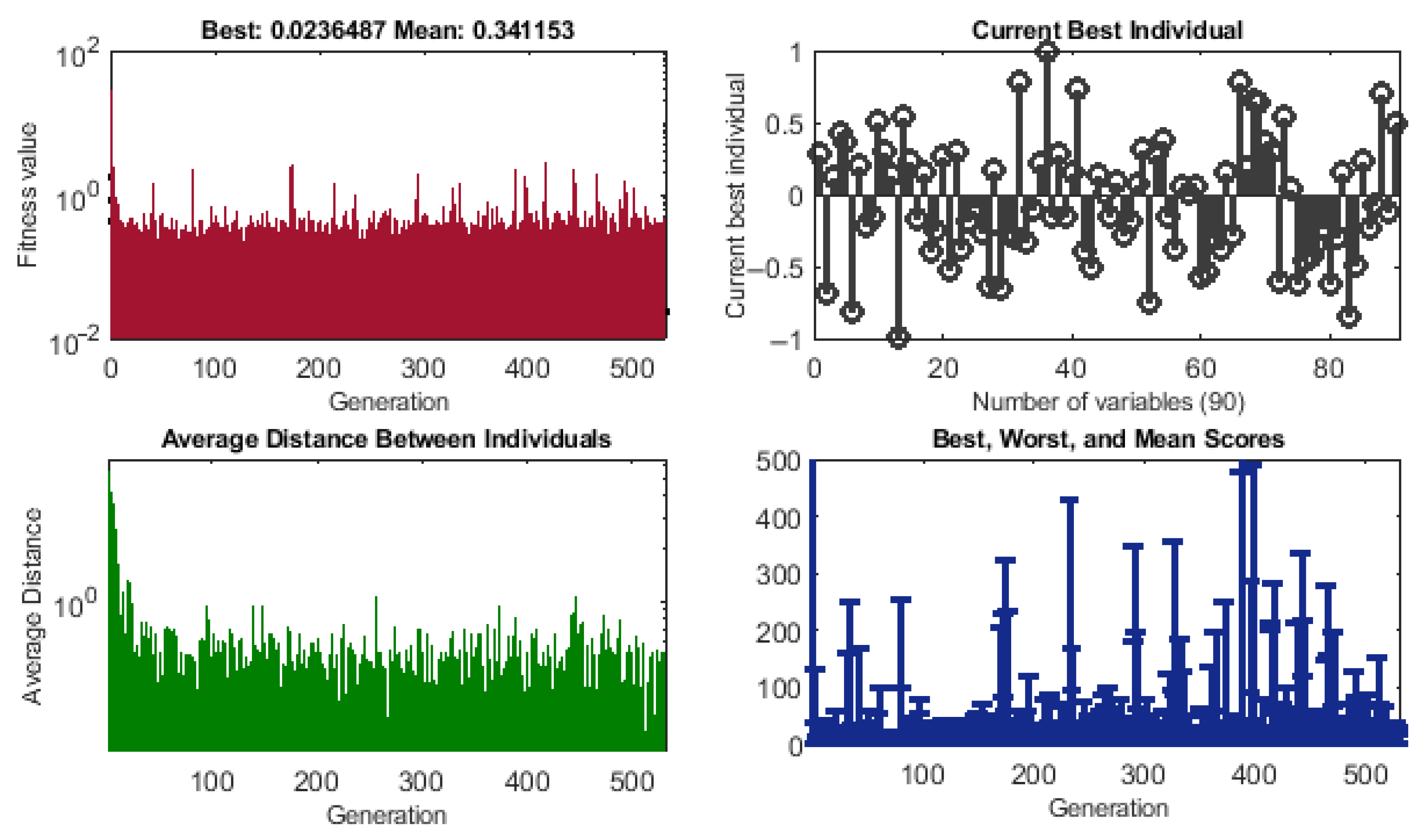
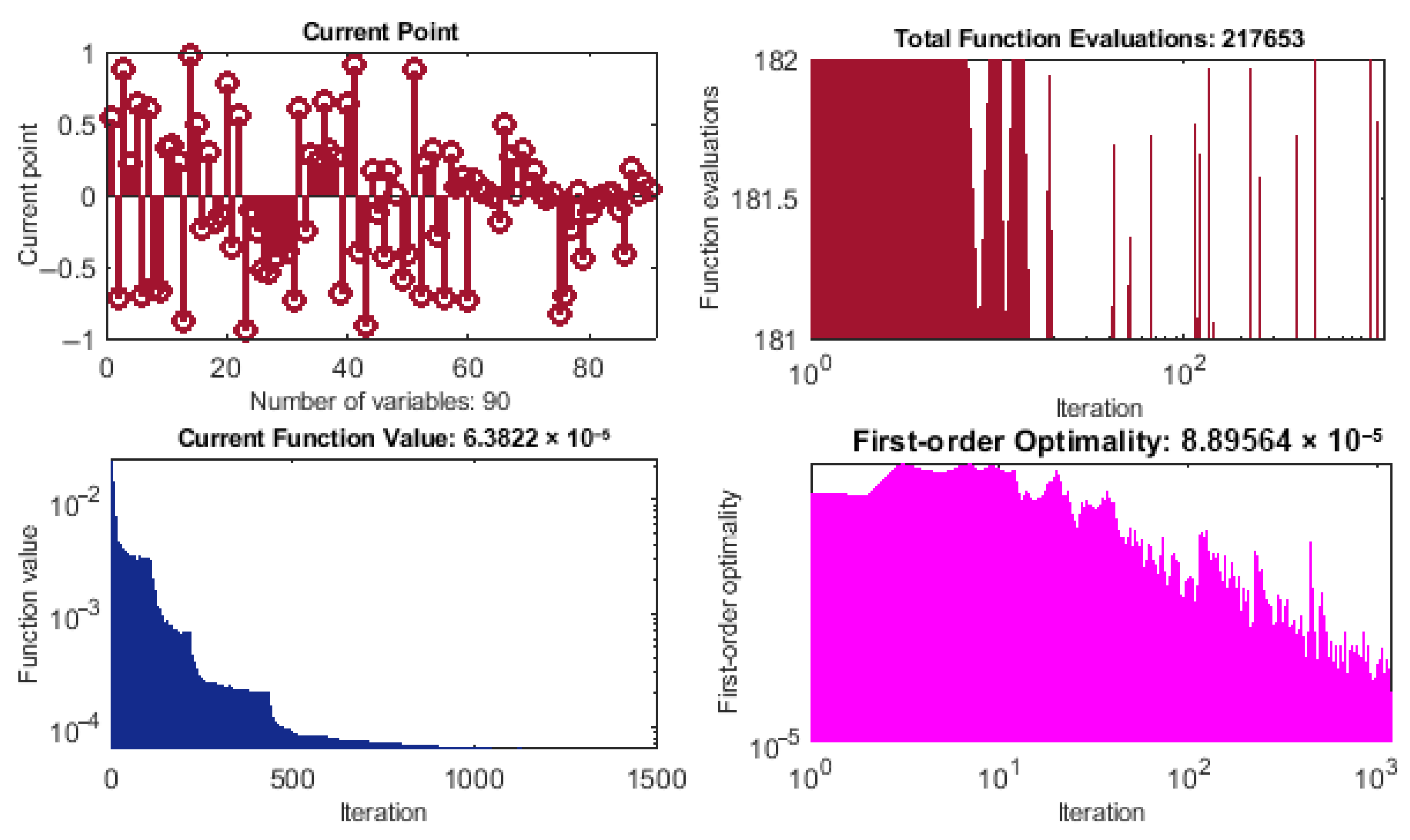
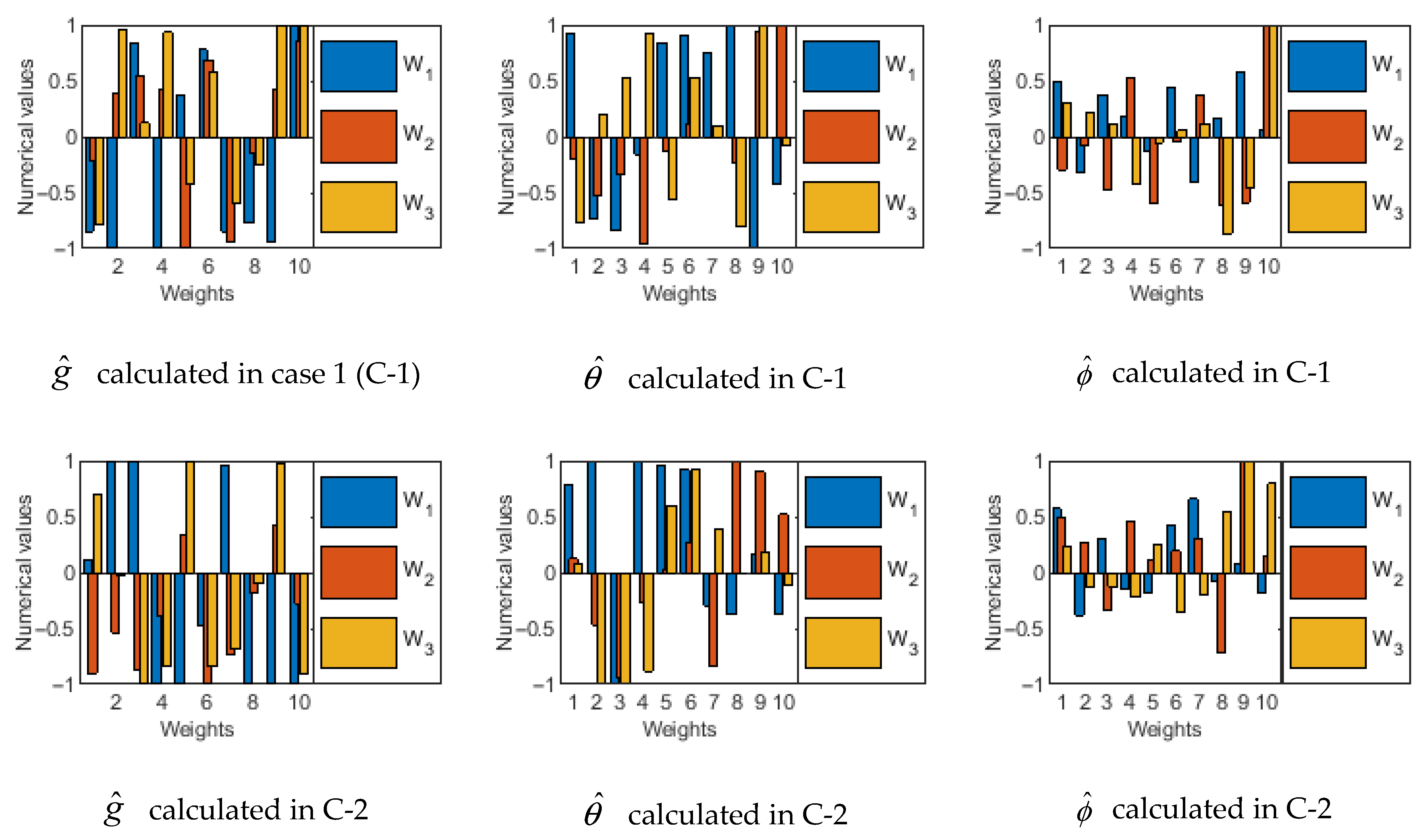
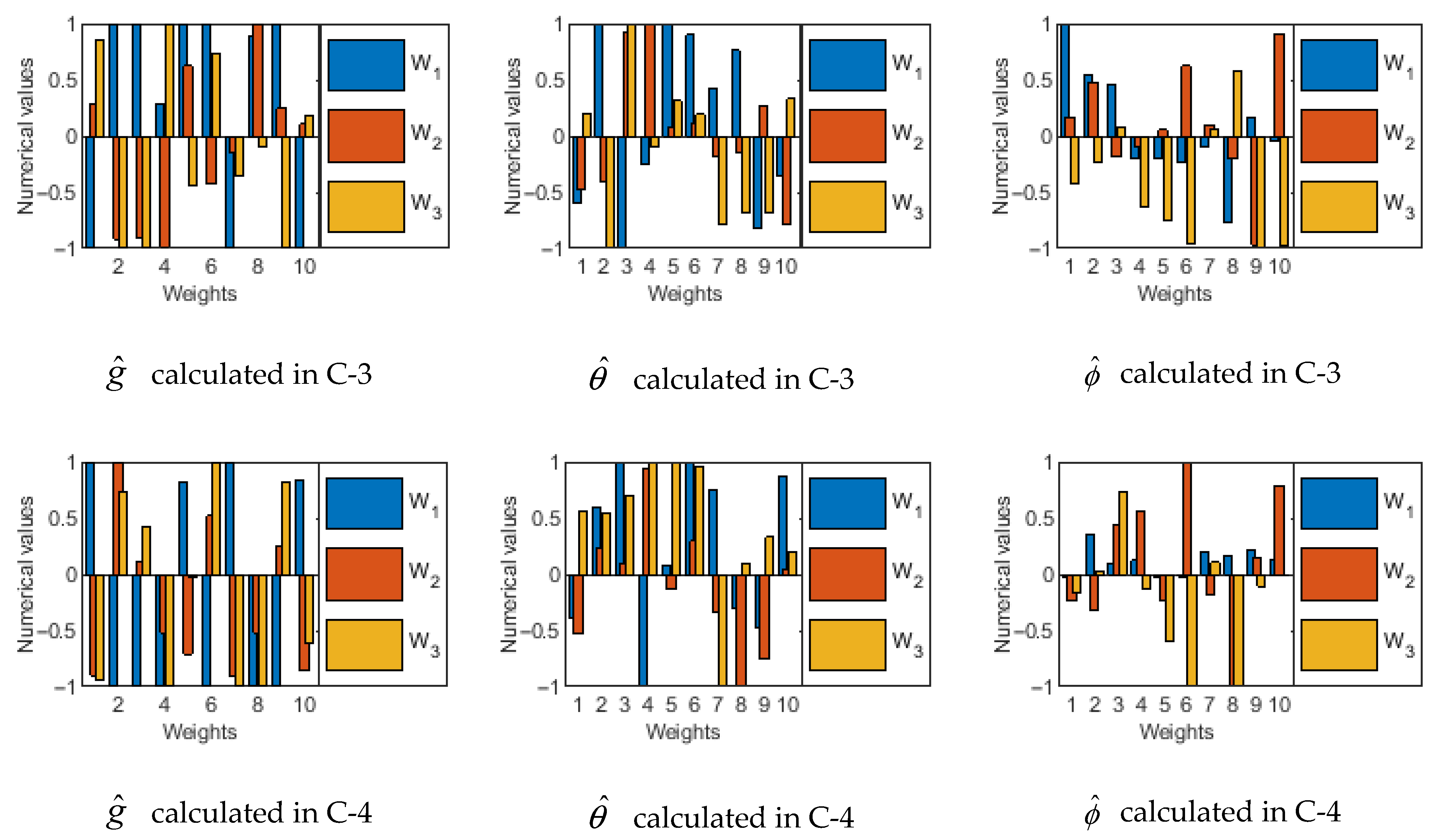
The HBI-RWNN solver was constructed to analyze the MHD-WNF-BL flow problem by solving the suggested problem in terms of a nonlinear ODE system on the interval [0, 5]. Six different scenarios, i.e., S(I–VI), were analyzed through physically existing parameters in the ODE system to obtain the approximate numerical outcomes of this problem in the shape of the velocity profile (η), temperature , and concentration . The required numerical solution of the MHD-WNF-BL problem was constructed using the unknown weights involved in it, which were first trained through the hybrid technique with the designed algorithm, and then the best-obtained weights were substituted into Equation (13) to obtain suitable numerical outcomes. Figure 3 demonstrates the learning process performed in the first case of S-I and the suitability of the hybrid technique involved in the HBI-RWNN algorithm, while the best-obtained weights in all cases of S-I in the MHD-WF-BL flow problem are illustrated in Figure 4.
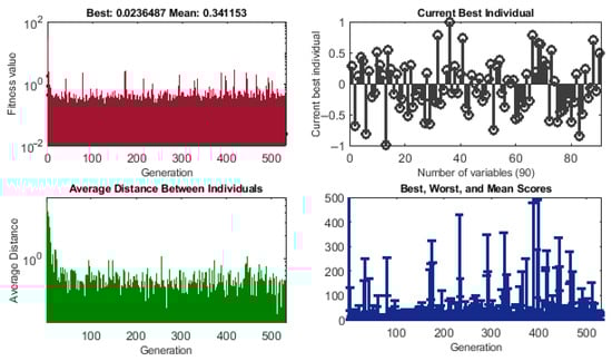

Figure 3.
HBI–RWNN solver was used to generate learning curve for case 1 (C-1) in scenario 1.
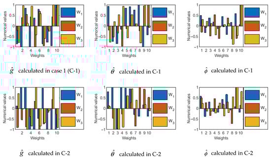
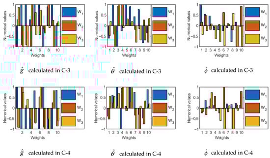
Figure 4.
Weights in C(1–4) in scenario 1 (S-I) calculated through HBI–RBNN solver for MHD–WNF–BL flow problem.
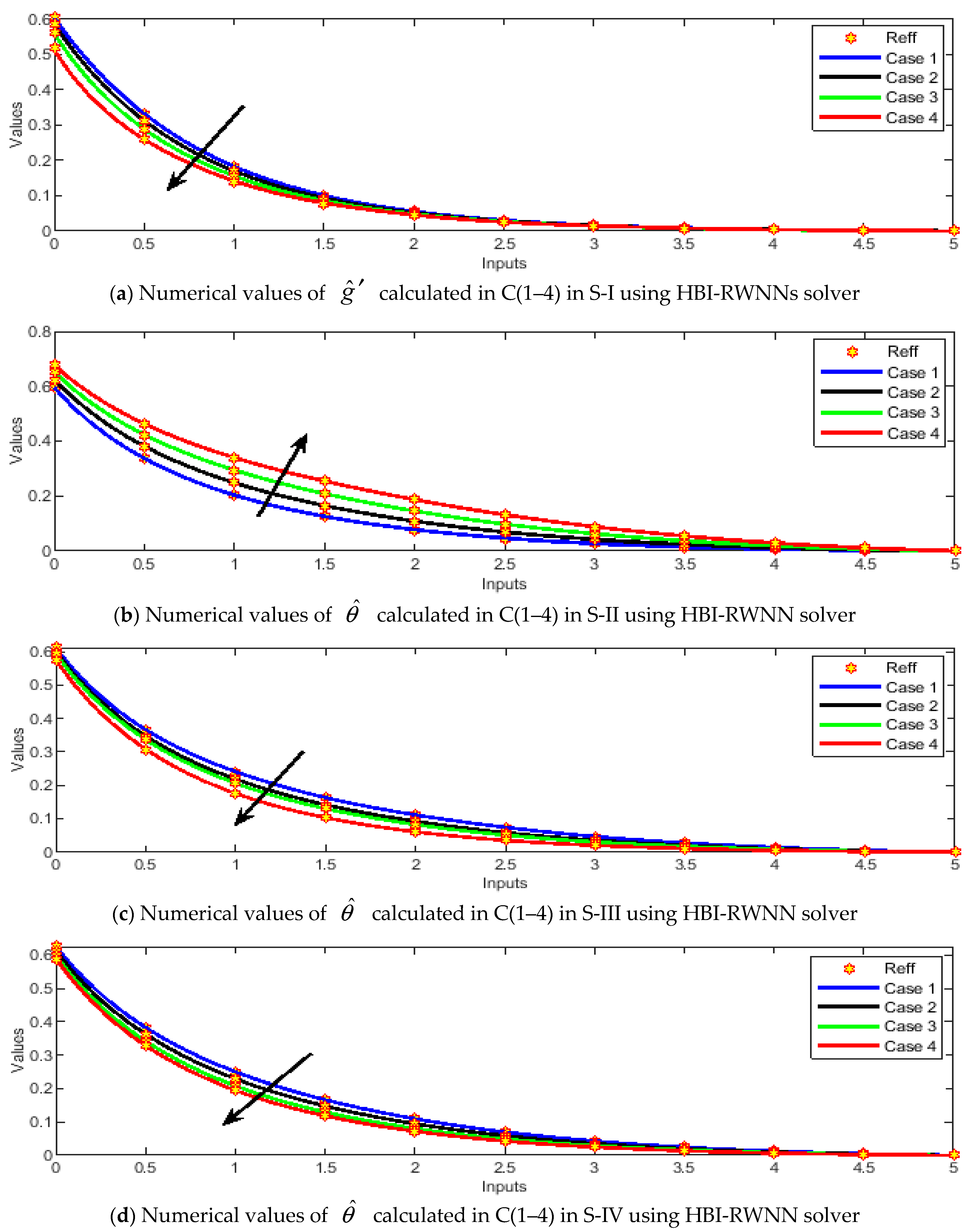
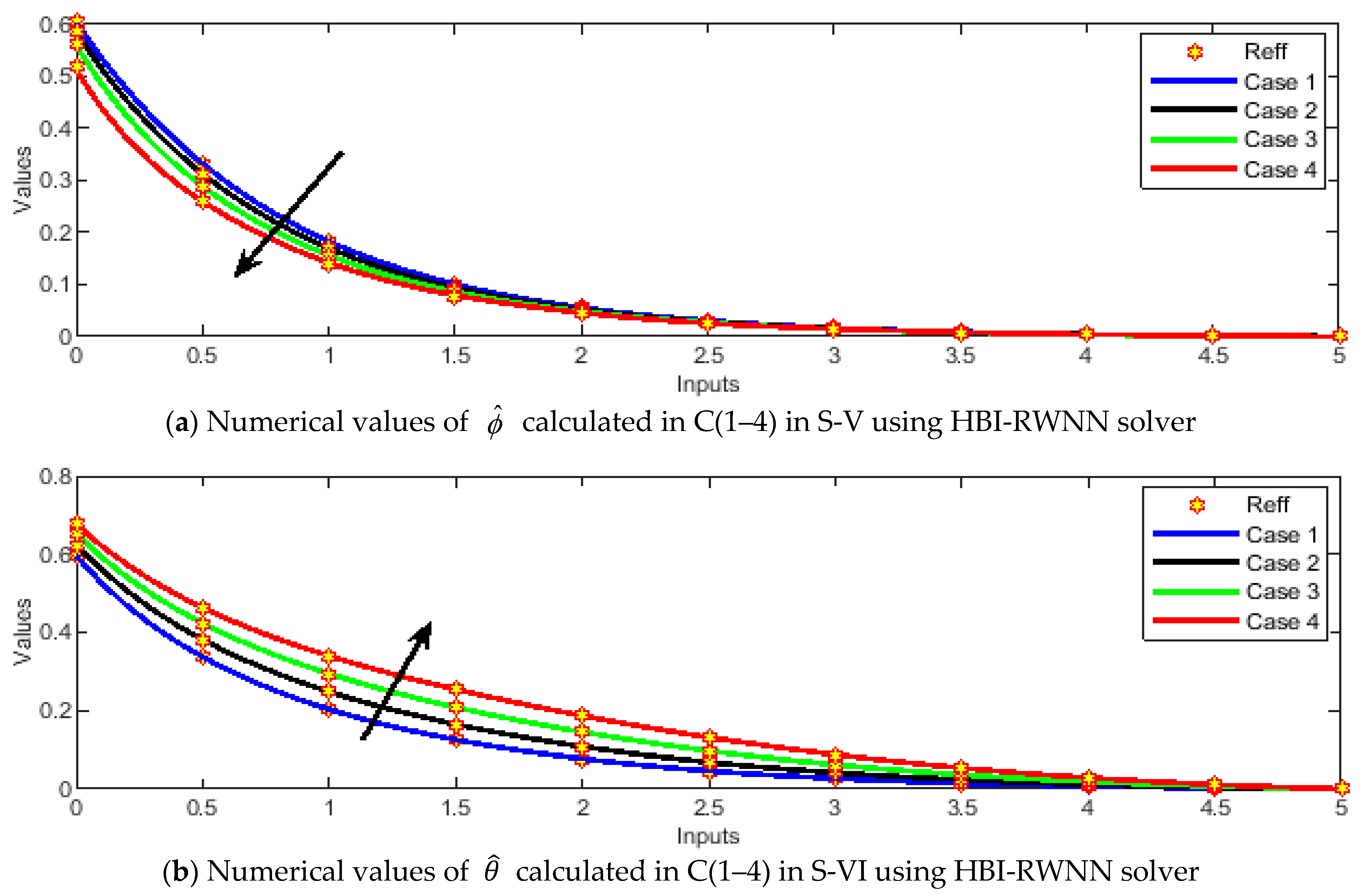
The numerical values of the MHD-WNF-BL flow problem in terms of velocity, temperature, and concentration using S(I–VI) are depicted as graphs in Figure 5 and Figure 6. Figure 5a indicates the influence of the Williamson parameter (λ) on and reveals that a larger value of λ reduces the boundary-layer thickness, and, as a result, the nanofluid velocity diminishes. Physically, a higher value of λ is a sign of a powerful shear-thinning attitude, which reduces the nanofluid flow. Figure 5b shows the relationship between the heat capacity ratio parameter (Nc) and temperature . In reality, a larger value of Nc escalates the thermal storage capacity, which allows the nanofluid to absorb a huge amount of heat energy through the stretchable surface, and temperature grows. Figure 5c,d illustrate the effect of the diffusivity ratio parameter (Nbt) and Lewis number (Le) on the thermal gradient. An increase in the value of both the Nbt and Le reduces the thermal BL width, and ultimately temperature decreases. Figure 6a demonstrates the effects of the Schmidt number (Sc) on . A larger Sc reduces the mass diffusivity, and, as a result, concentration decreases. Figure 6b shows the effects of the thermal slip parameter (Z4) on temperature. A surge in the value of Z4 reduces the thermal BL width, and consequently diminishes.
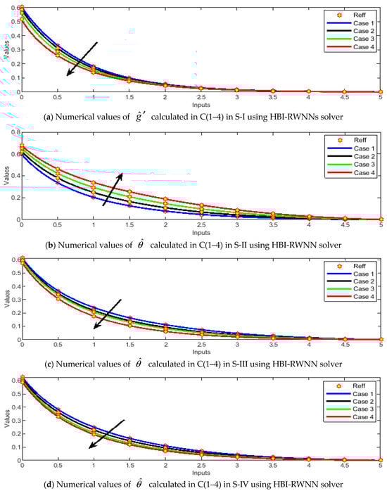
Figure 5.
Numerical values calculated in S(I–IV) using HBI-RWNN solver for MHD-WNF-BL flow problem.
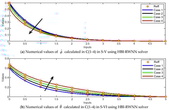
Figure 6.
Numerical values calculated in S(V–VI) using HBI-RWNN solver for MHD-WNF-BL flow problem.
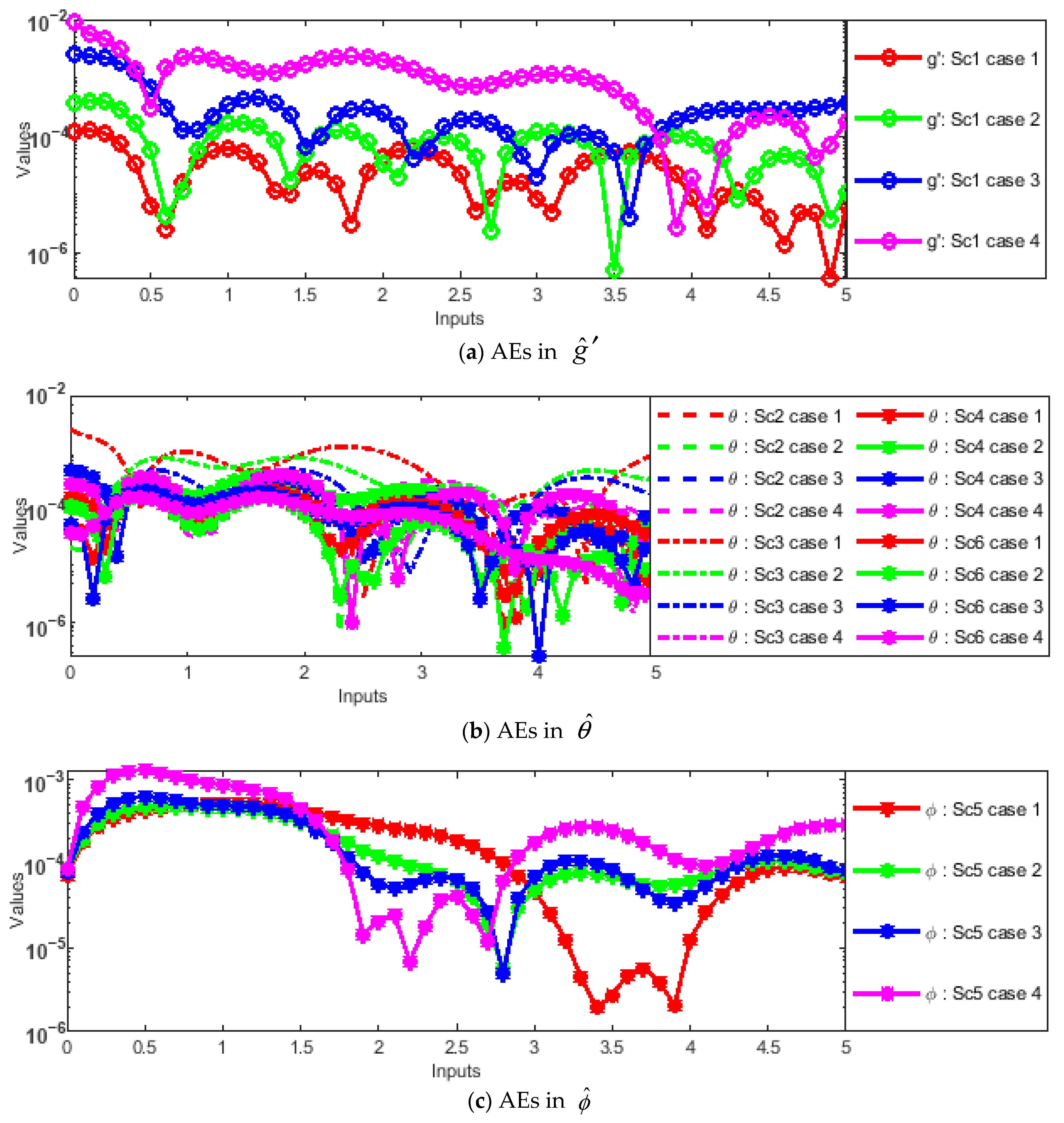
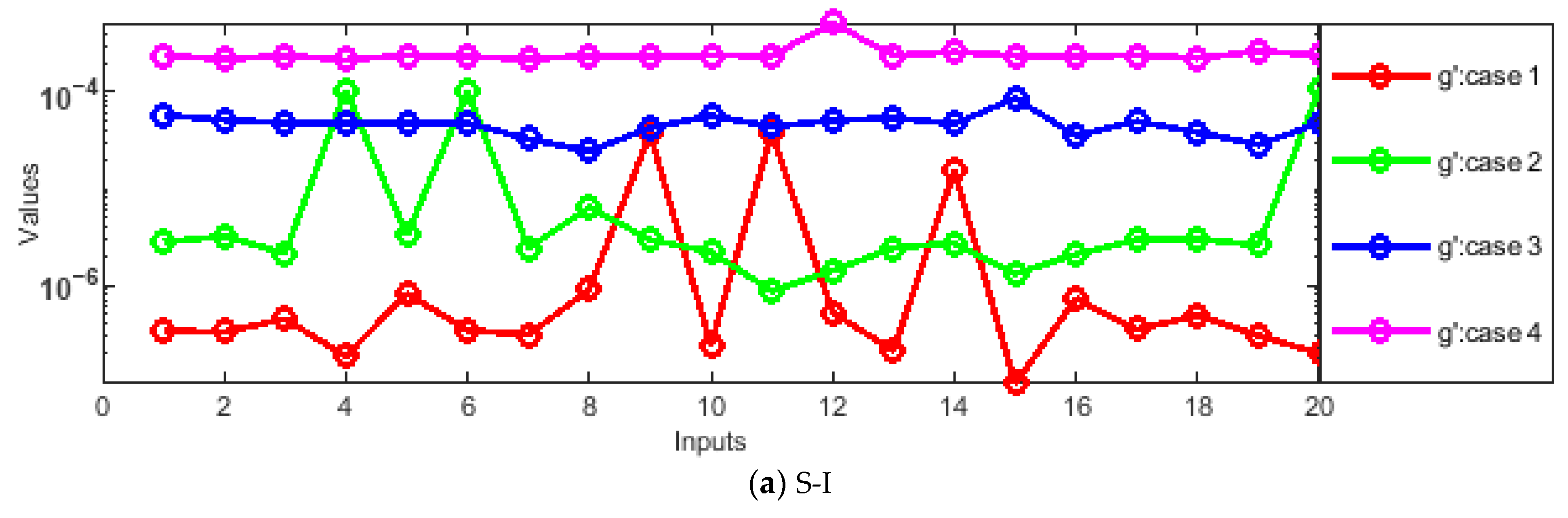
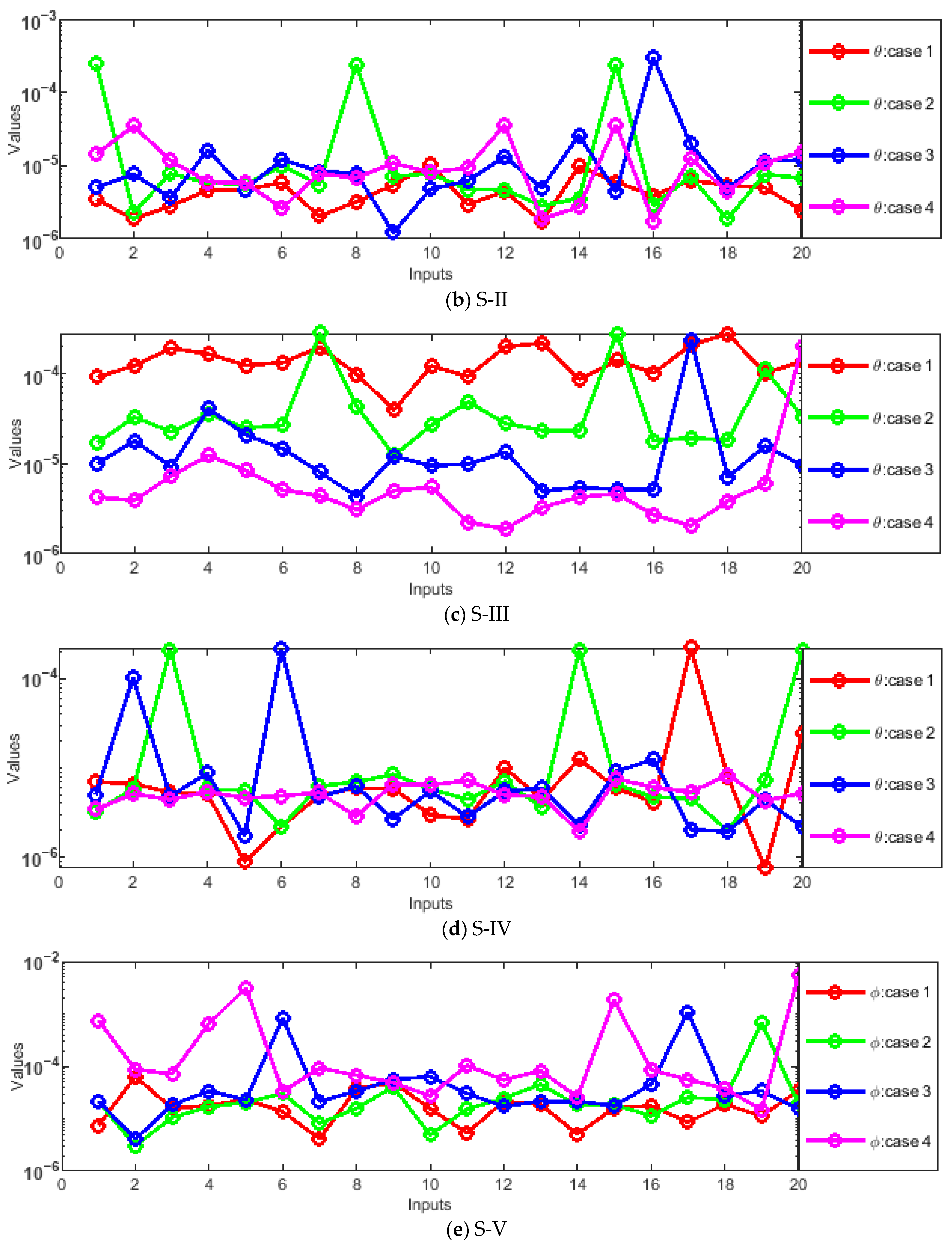
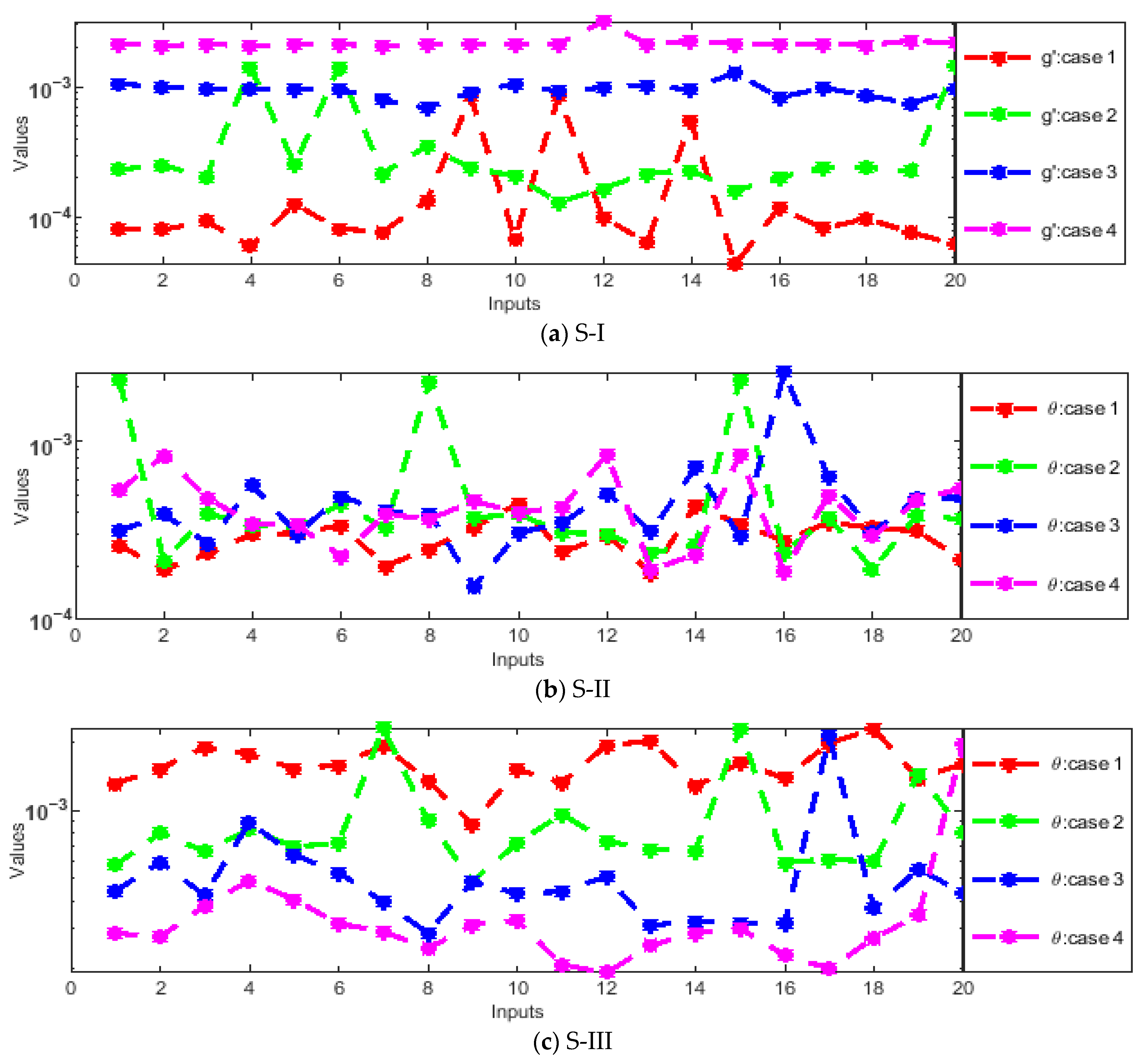
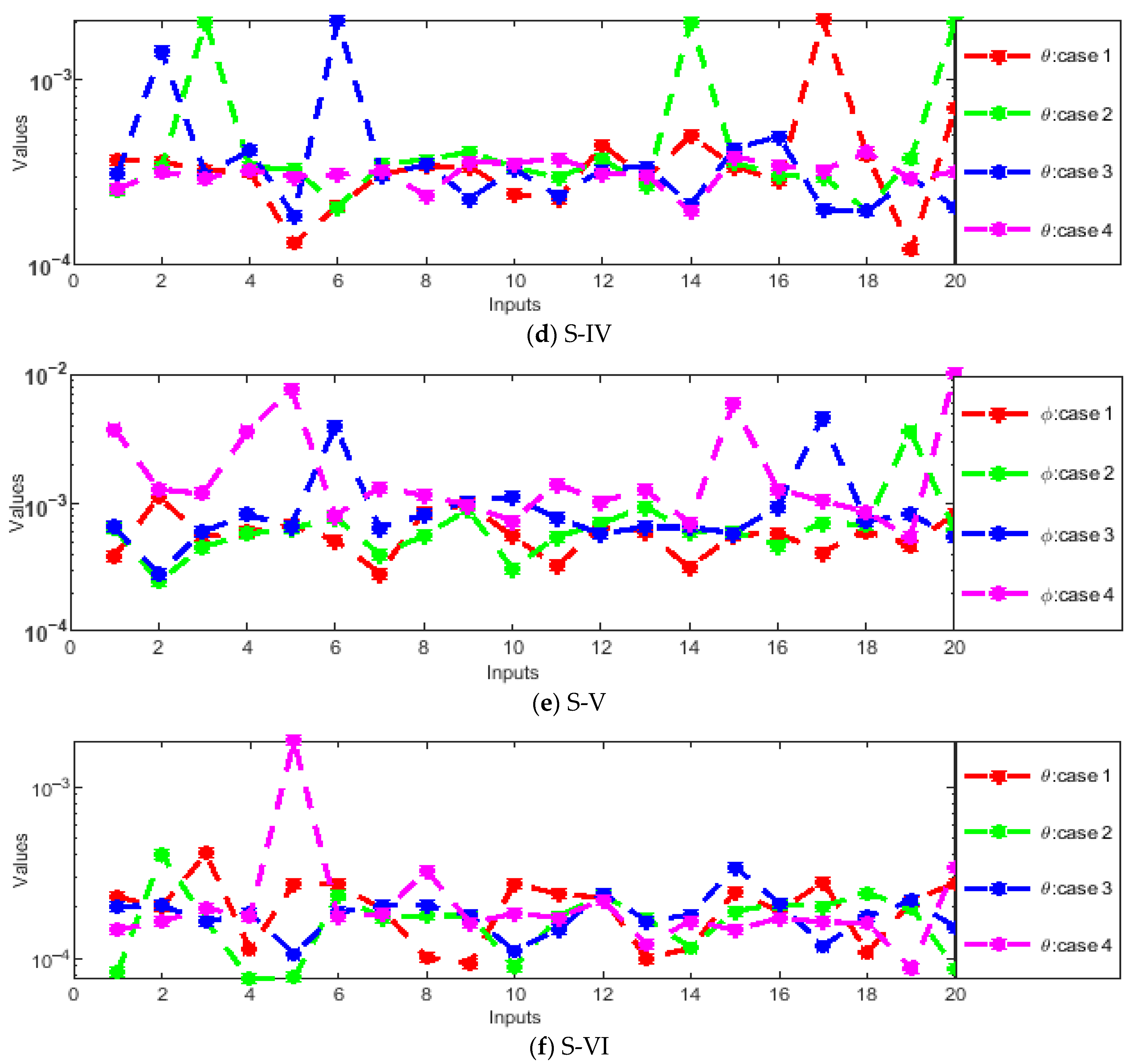
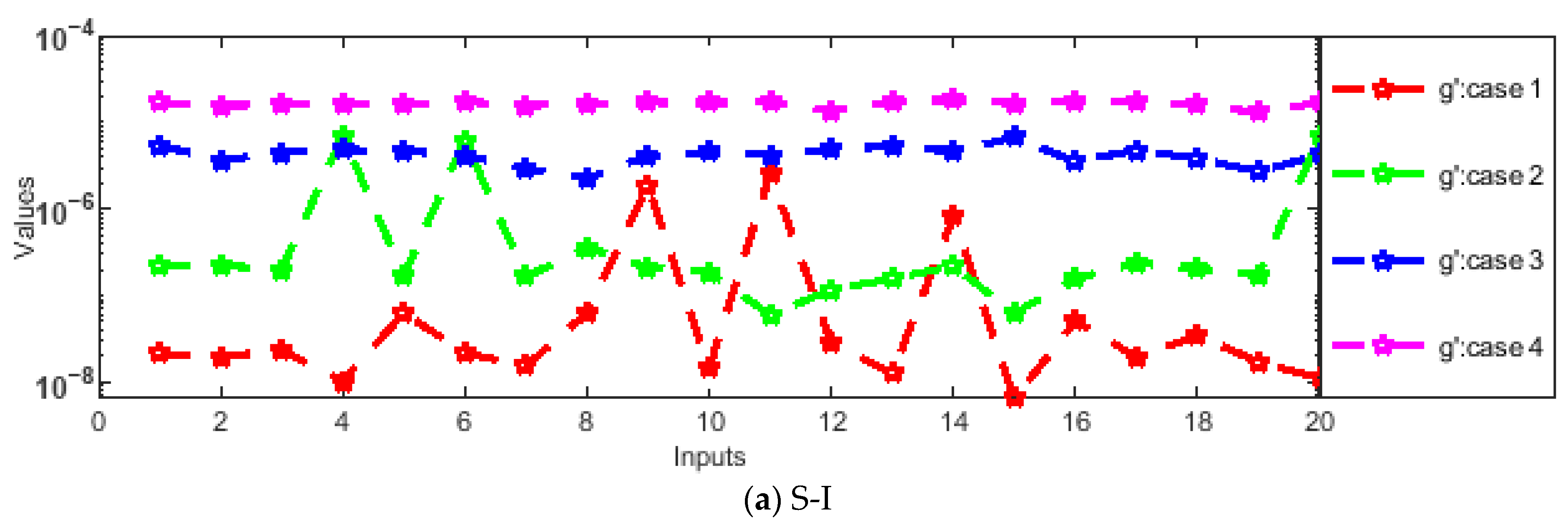
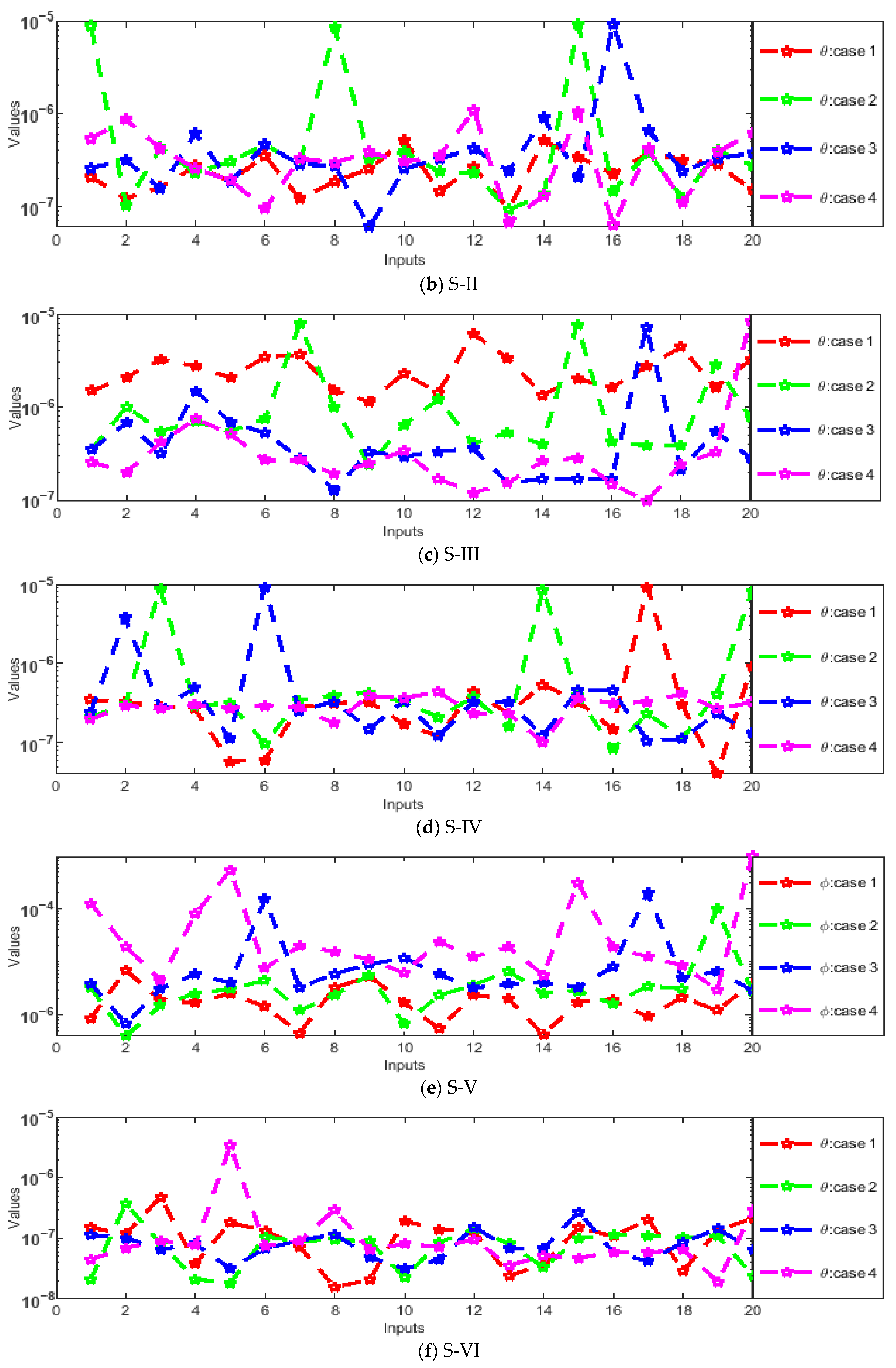
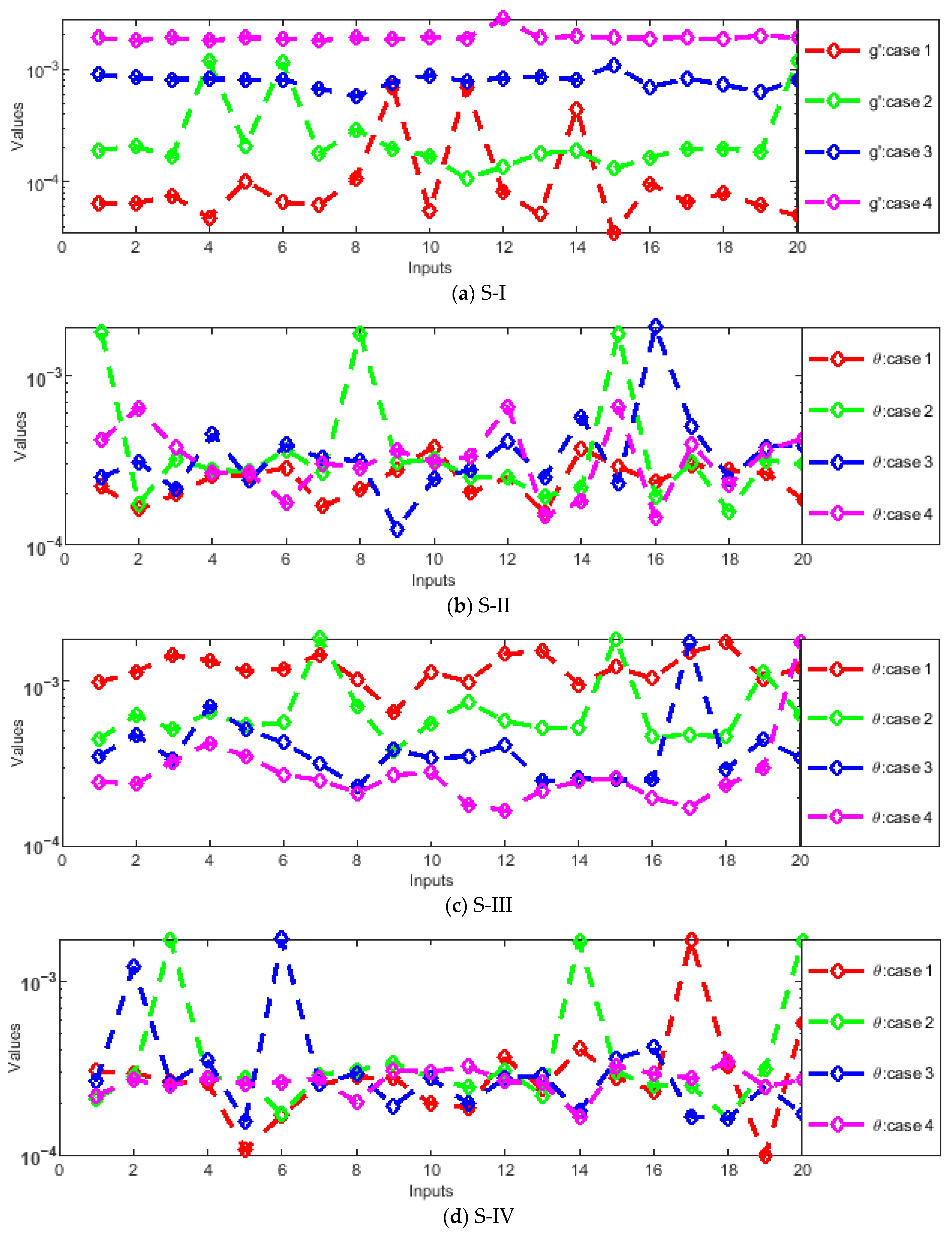
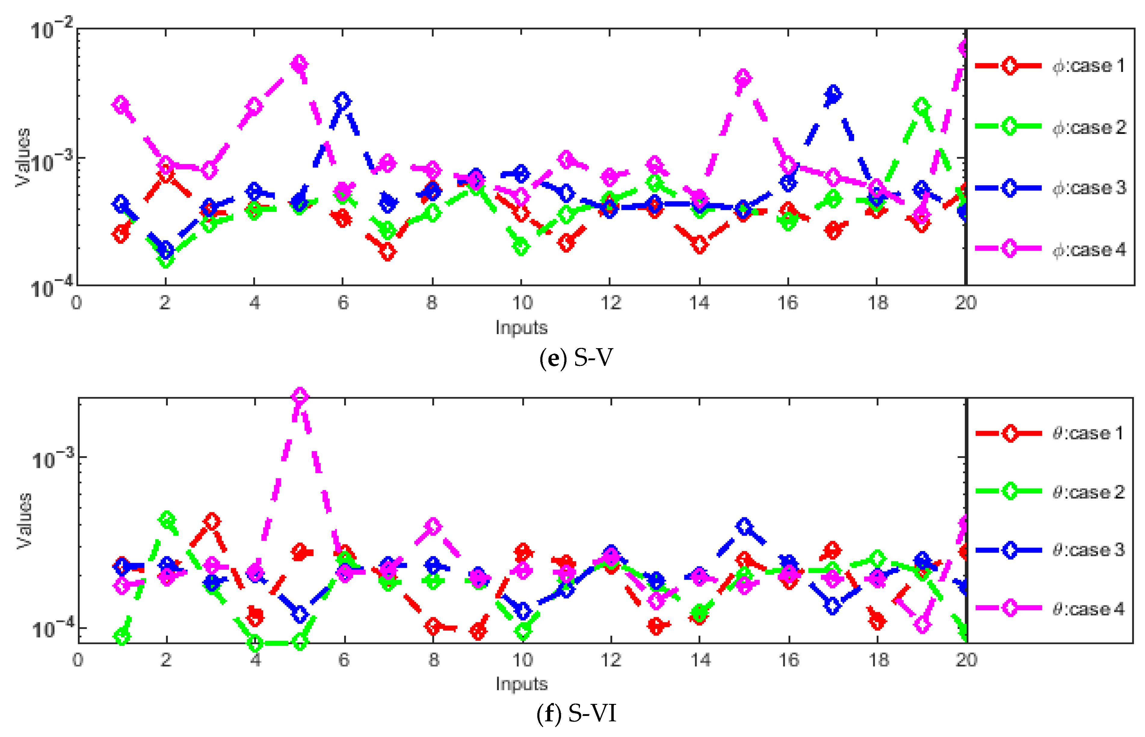
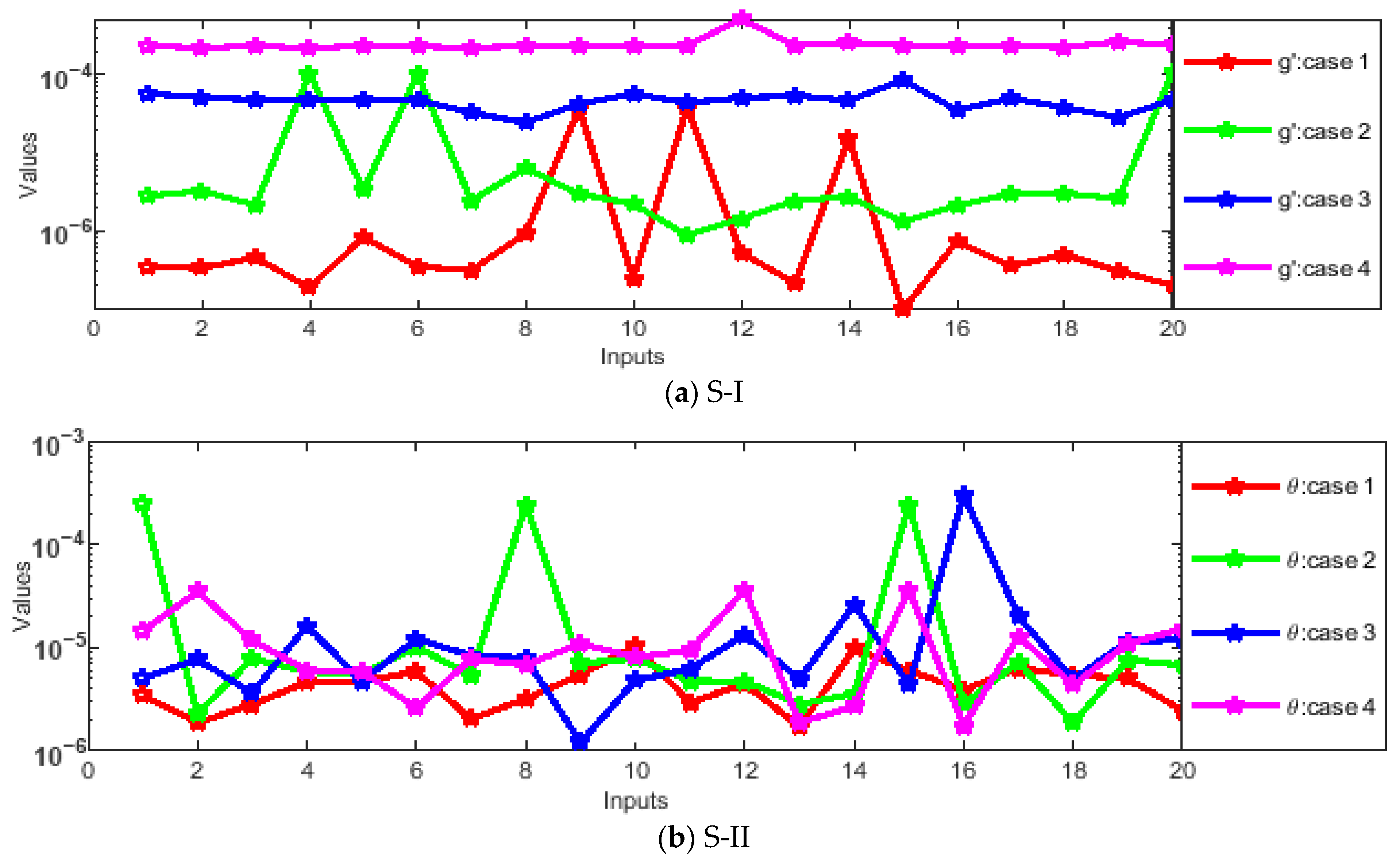
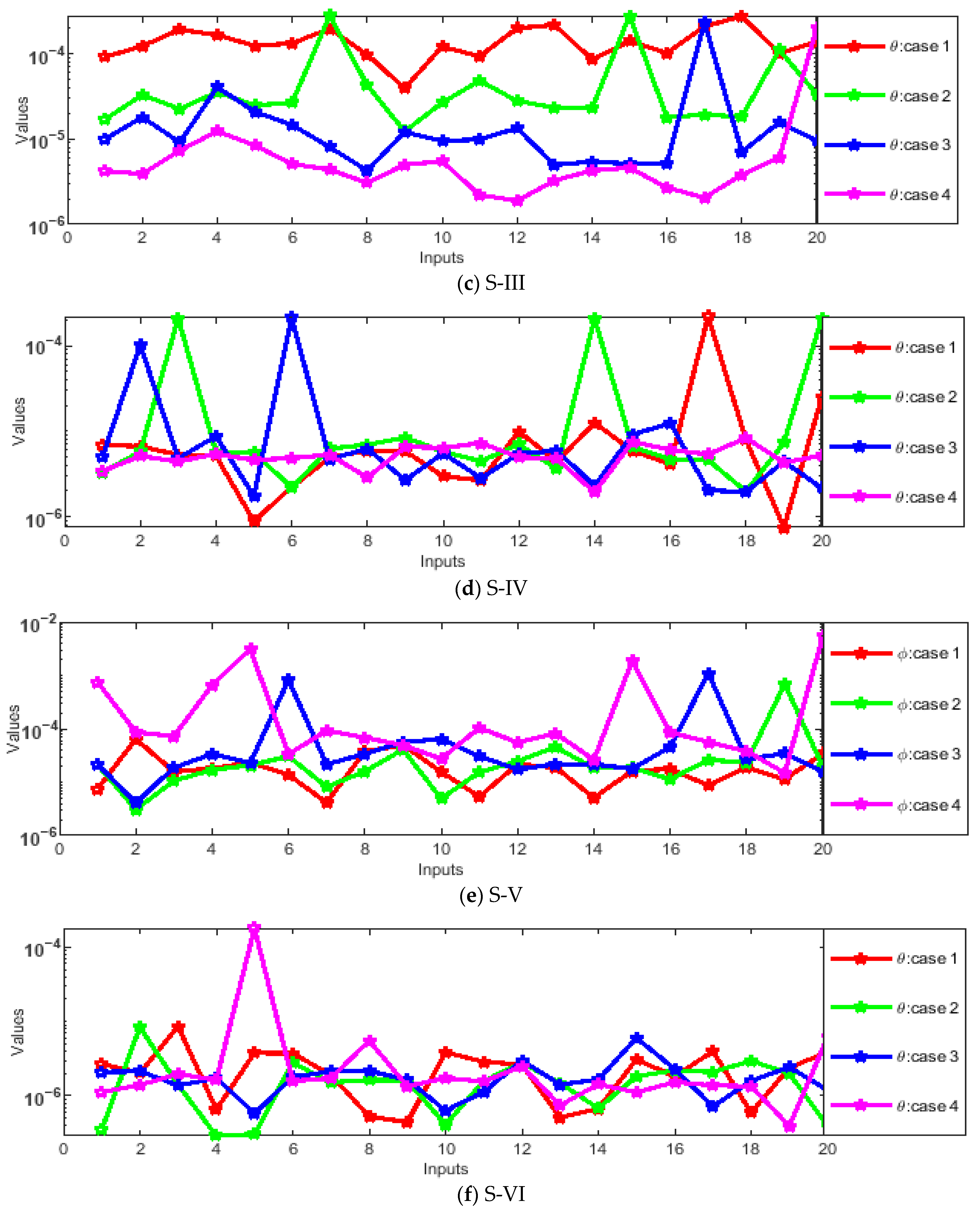
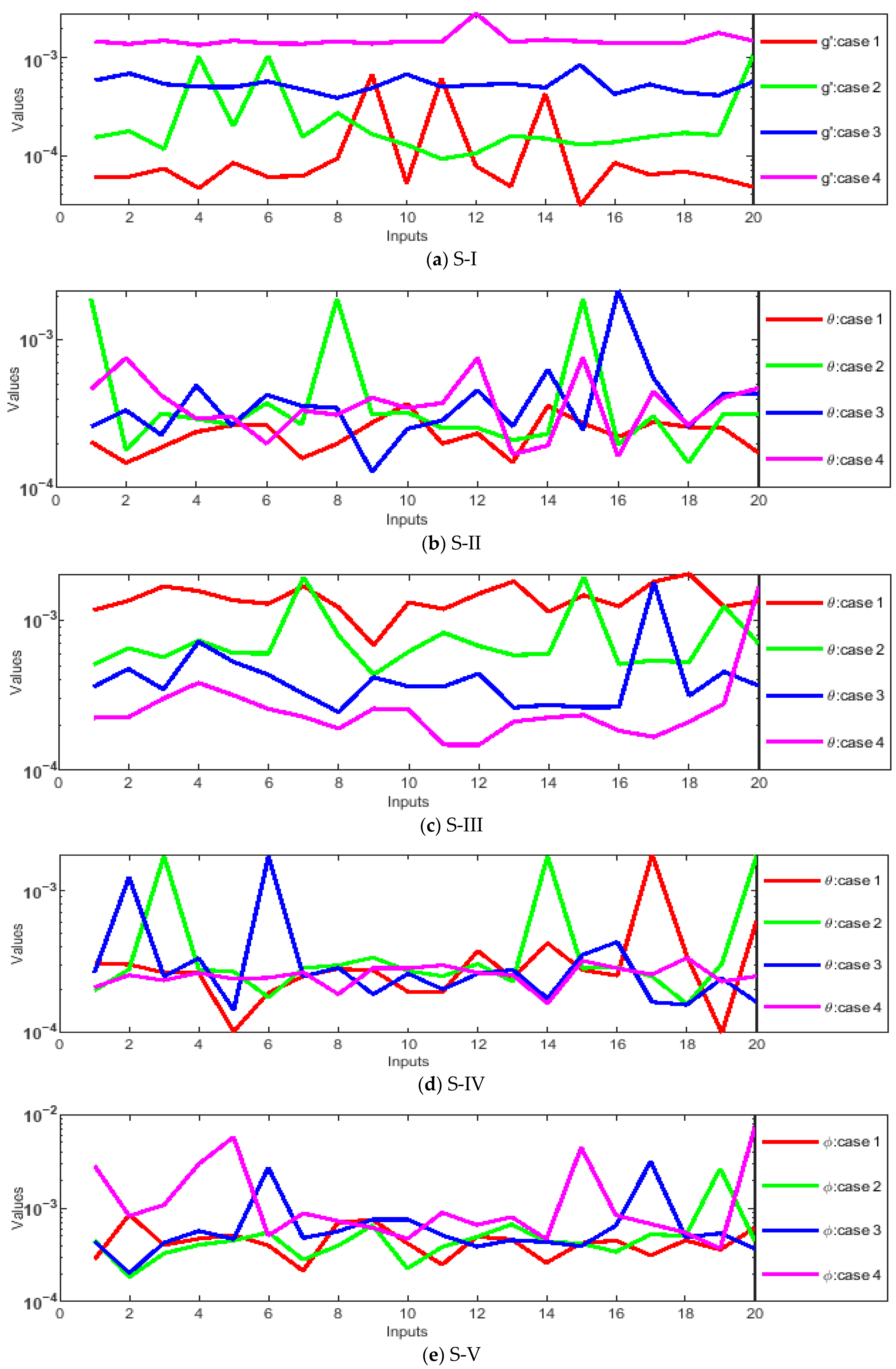
The numerically results of the MHD-WNF-BL flow problem calculated using the HBI-RWNN algorithm successfully matched the reference results, and Figure 7 illustrates their comparison in terms of the graphs obtained in all scenarios (S(I–VI)). The results obtained for , , and lay in a range of accuracy 10−2 ↔ 10−6 (up to five decimals), 10−2 ↔ 10−6, and 10−3 ↔ 10−6, respectively, in S(I–VI), which indicate the suitability of the designed solver. Table 3 and Table 4 demonstrate the AEs calculated in cases C(1–4) of all scenarios S(I–VI) for the interval [0, 5].
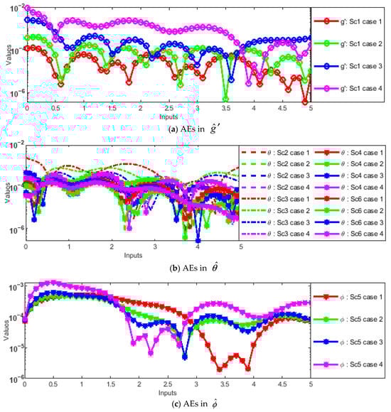
Figure 7.
AEs calculated in S(I–VI) for MHD–WNF–BL flow problem using HBI–RWNN solver.
Table 3.
AEs in S(I–IV) for MHD-WNF-BL flow problem calculated via HBI-RWNN solver.
Table 4.
AEs of S(V–VI) for MHD-WNF-BL flow problem calculated via HBI-RWNN solver.
Moreover, the stability of the designed HBI-RWNN solver was determined by various statistical performance operators, and the obtained graphs are presented in Figure 8, Figure 9, Figure 10, Figure 11, Figure 12 and Figure 13. The range of accuracy in S(I–VI) obtained from the analyses of E-NSE, RMSE, E-VAF, E-TIC, E-R2, and MAE are, respectively, 10−3 ↔ 10−7, 10−2 ↔ 10−4, 10−4 ↔ 10−9, 10−3 ↔ 10−4, 10−3 ↔ 10−7 and 10−3 ↔ 10−4 for S-I, 10−3 ↔ 10−6, 10−2 ↔ 10−4, 10−5 ↔ 10−7, 10−3 ↔ 10−4, 10−3 ↔ 10−6, and 10−3 ↔ 10−4 for S-II 10−4 ↔ 10−6, 10−2 ↔ 10−4, 10−5 ↔ 10−7, 10−3 ↔ 10−4, 10−4 ↔ 10−6, and 10−3 ↔ 10−4 for S-III; 10−4 ↔ 10−6, 10−3 ↔ 10−4, 10−5 ↔ 10−7, 10−3 ↔ 10−4, 10−4 ↔ 10−6, and 10−3 ↔ 10−4 for S-IV; 10−2 ↔ 10−6, 10−2 ↔ 10−4, 10−3 ↔ 10−7, 10−2 ↔ 10−4, 10−2 ↔ 10−6, and 10−2 ↔ 10−4 for S-V; 10−4 ↔ 10−7, 10−3 ↔ 10−4, 10−5 ↔ 10−8, 10−3 ↔ 10−4, 10−4 ↔ 10−7, and 10−3 ↔ 10−4 for S-VI. Table 5 and Table 6 demonstrate the best values calculated in all C(1–4) in S(I–VI) using the above-stated statistics, and the obtained accuracy confirms the suitability of the designed solver to handle stiff nonlinear problems similar to the MHD-WNF-BL fluid model.
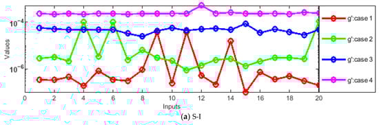
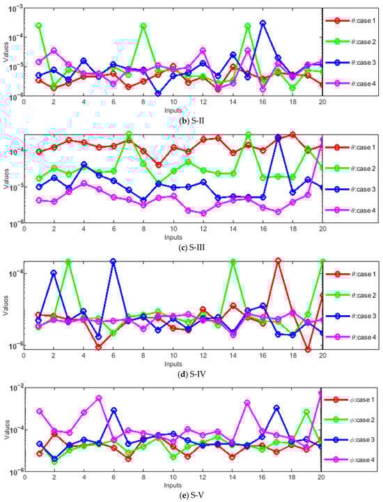
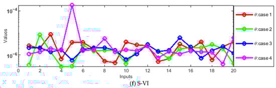
Figure 8.
E-NSE analysis of S(I–VI) for MHD–WNF–BL flow problem using HBI–RWNN solver.

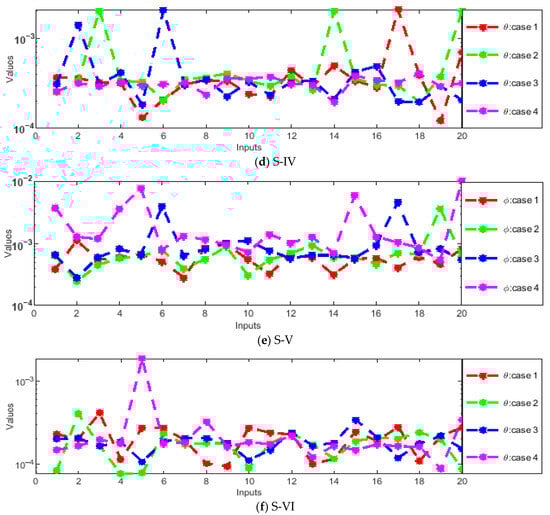
Figure 9.
RMSE analysis of S(I–VI) for MHD–WNF–BL flow problem using HBI-RWNN solver.
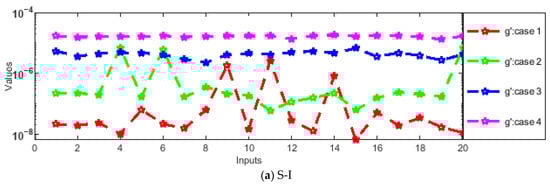
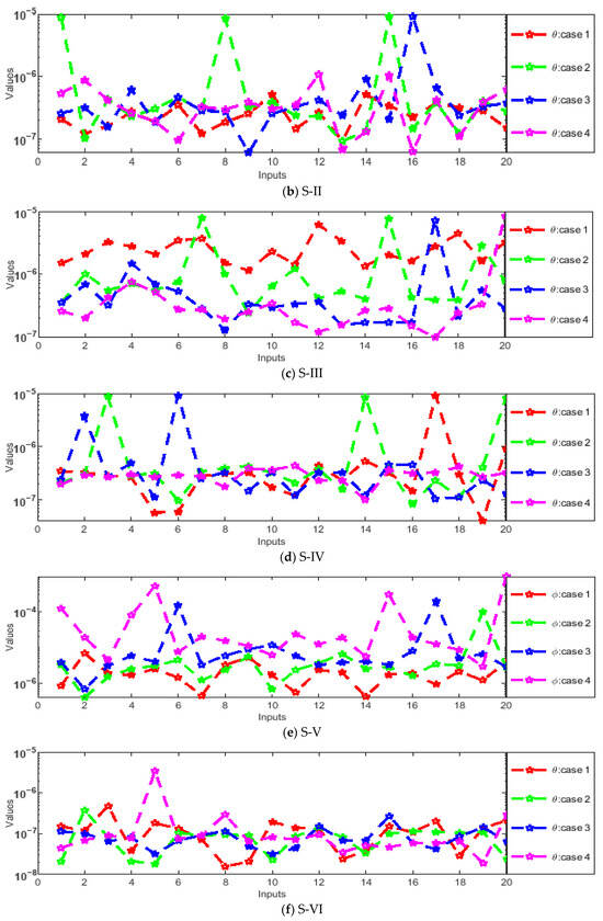
Figure 10.
E-VAF analysis of S(I–VI) for MHD–WNF–BL flow problem using HBI–RWNN solver.
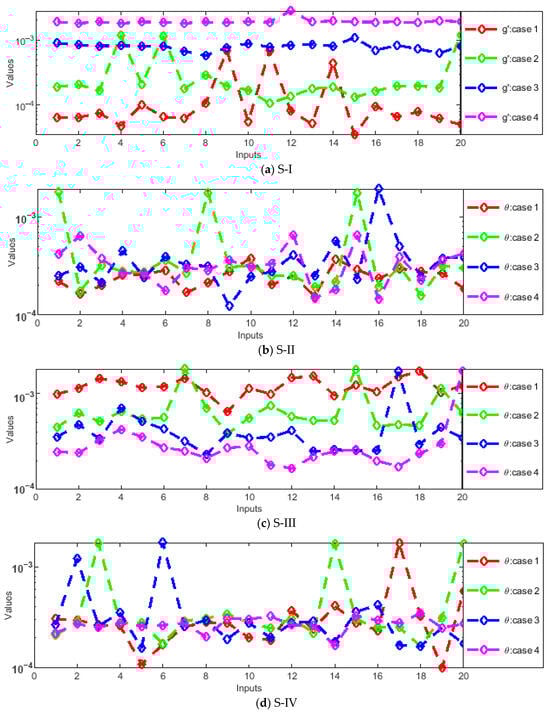
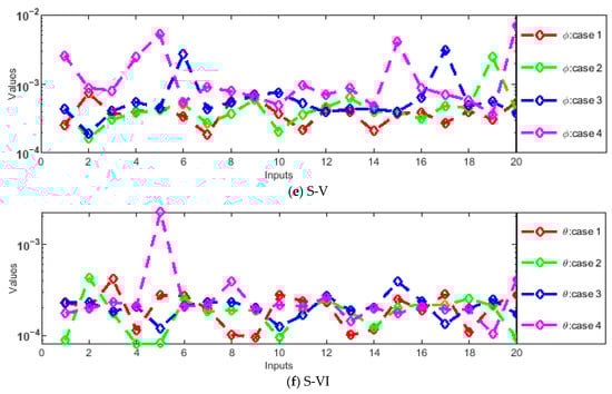
Figure 11.
E-TIC analysis of S(I–VI) for MHD–WNF–BL flow problem using HBI–RWNN solver.
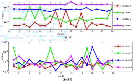
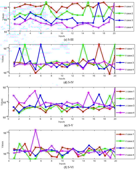
Figure 12.
E-R2 analysis of S(I–VI) for MHD–WNF–BL flow problem using HBI–RWNN solver.
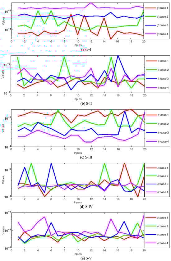
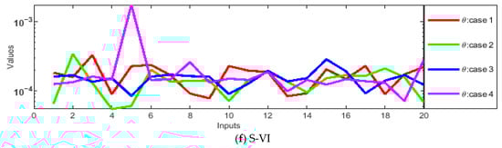
Figure 13.
MAE analysis of S(I–VI) for MHD–WNF–BL flow problem using HBI–RWNN solver.
Table 5.
Best statistical-operators-based values for S(I–II) using HBI-RWNN solver.
Table 6.
Best statistical-operators-based values for S(III–VI) using HBI-RWNN solver.
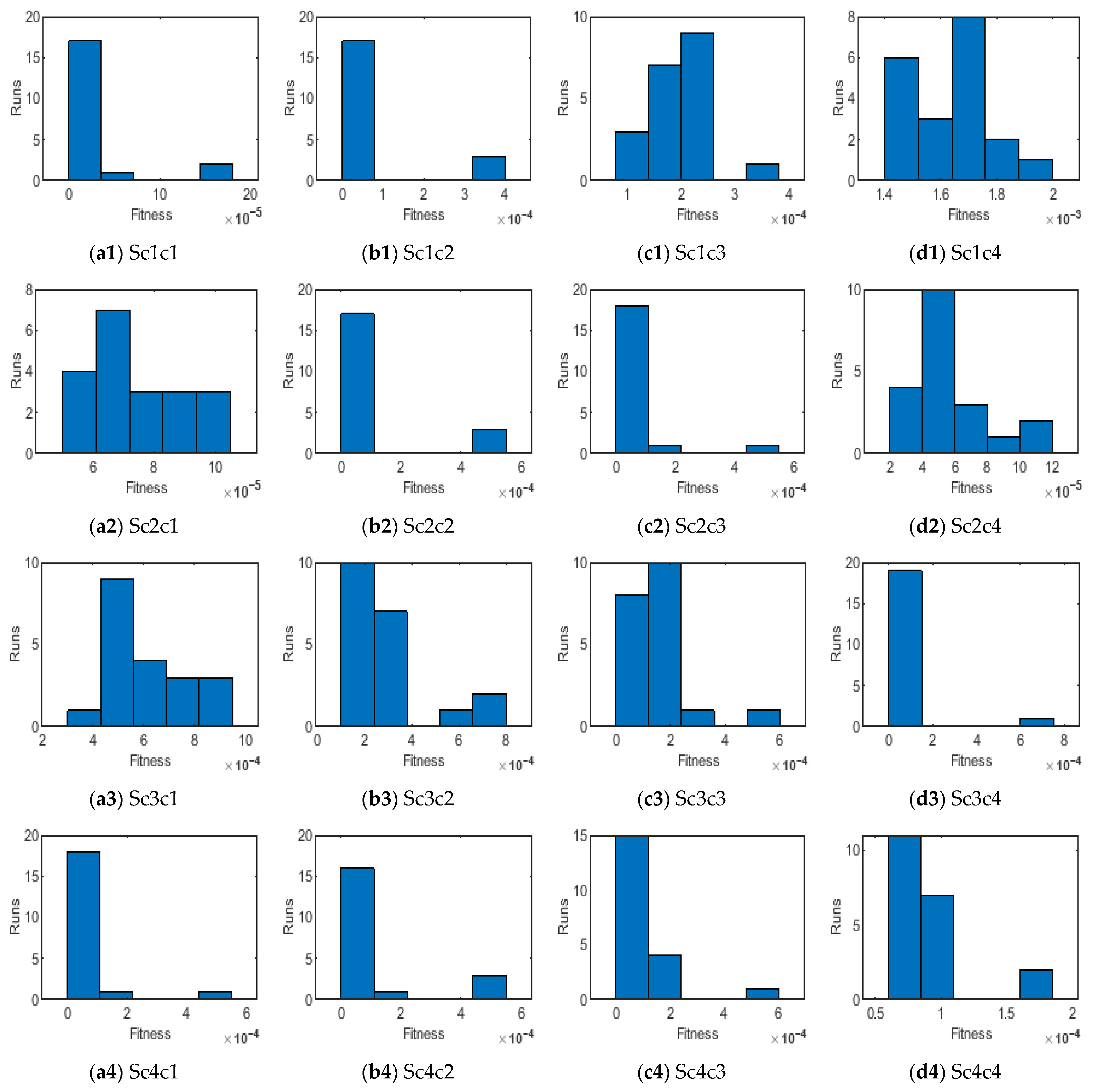
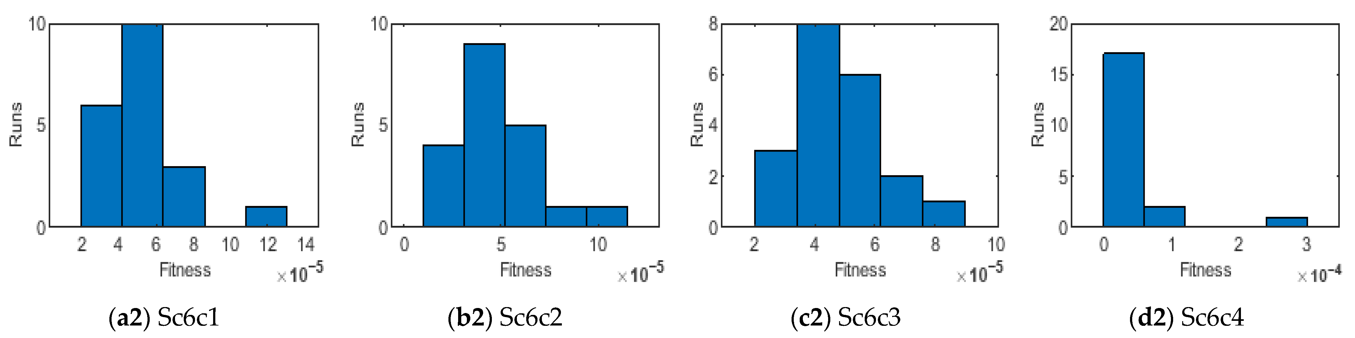
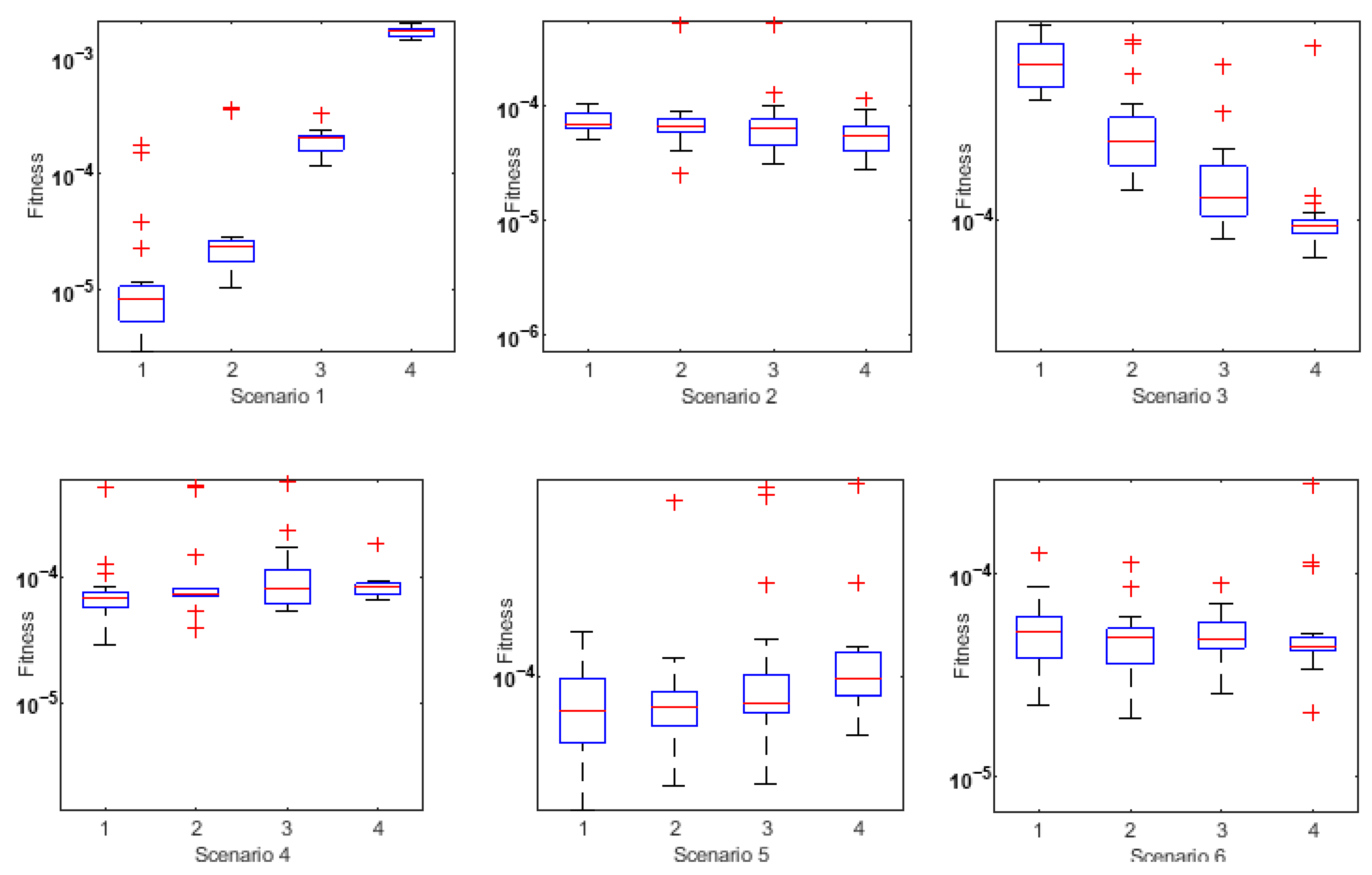
Furthermore, the performance of the designed HBI-RWNN solver was comprehensively verified through histogram and box -plot analyses of all cases (C(1–4)) of S(I–VI), and the obtained plots are shown in Figure 14, Figure 15 and Figure 16. Figure 14 and Figure 15 demonstrate the histogram analysis in all cases (C(1–4)) of the discussed scenarios, having an accuracy range of 10−3 ↔ 10−4 for S-I, 10−4 ↔ 10−5 for S-II, 10−3 ↔ 10−4 for S-III, and 10−4 ↔ 10−5 for S-IV, S-V, and S-VI, which shows that almost 80% of the total runs attained stiff criteria in the accuracy range of 10−4 ↔ 10−5. Figure 16 depicts the box-plot analyses for all cases of S(I–VI), and the obtained accuracy in all scenarios is up to 10−6 (up to five decimals), which proves the tendency of the designed solver to achieve highly accurate results for stiff nonlinear problems.
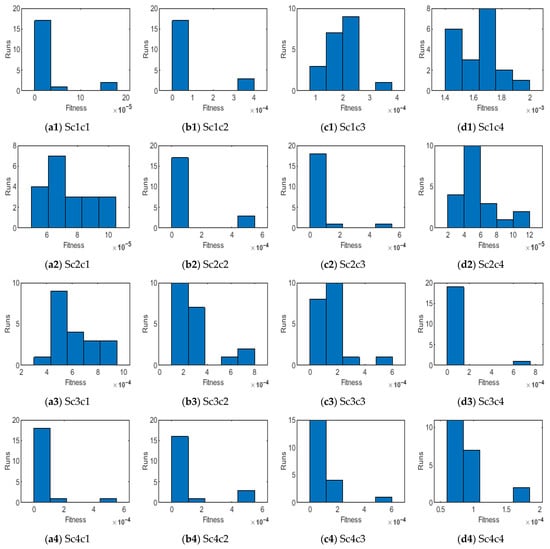
Figure 14.
Histogram analysis of C(1–4) in S(I–V) using HBI–RWNN solver.
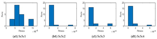
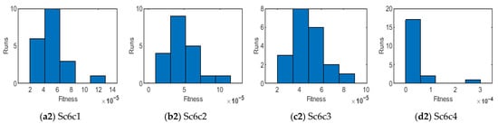
Figure 15.
Histogram analysis of C(1–4) in S(V–VI) using HBI–RWNN solver.
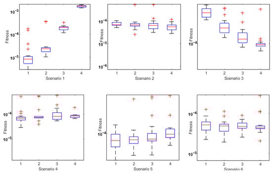
Figure 16.
Histogram analysis of C(1–4) in all scenarios using HBI–RWNN solver.
5. Conclusions
A newly designed HBI-RWNN solver was applied to solve the MHD-WNF-BL flow problem in terms of a nonlinear system of ODEs using scenarios S(I–VI), each containing four different cases. The obtained numerical results in terms of velocity profile, thermal gradient, and concentration of nanofluid were successfully compared with the pre-calculated reference results of the suggested problem. The AEs calculated in each scenario were depicted in graphs and tables. The detailed form of the stability and performance analyses of the HBI-RWNN solver were also presented in graphical and tabulated forms. The major outcomes of this research are defined below:
- An increase in the value of Williamson parameter diminishes the nanofluid velocity.
- The consequences of the diffusivity ratio parameter, Lewis number, and thermal slip parameter on the thermal gradient profile are identical, but a reciprocal effect is observed in case of the heat capacity ratio parameter.
- An escalation in the value of the Schmidt parameter reduces the nanofluid concentration.
- The designed solver optimized through the hybrid GA-SQP approach achieves exceptionally low AEs, consistently in the order of 10−7 ↔ 10−9, confirming the excellent precision and reliability of the proposed numerical framework.
The overall error analysis strongly indicates that the hybridized intelligent solver not only accelerates convergence but also maintains efficacy, thus offering a highly effective and practical tool for solving complex nonlinear boundary-layer flow problems.
Author Contributions
Conceptualization, I.A. and M.A.Z.R.; methodology, Z.I.B. and S.I.H.; software, M.S. and Z.I.B.; validation, M.A.Z.R. and R.K.; formal analysis, M.S. and Z.I.B.; investigation, I.A. and S.I.H.; resources, M.A.Z.R. and M.S.; data curation, S.I.H.; writing—original draft preparation, Z.I.B.; writing—review and editing, Z.I.B. and S.I.H.; visualization, M.S.; supervision, I.A.; project administration, I.A. and M.A.Z.R.; funding acquisition, S.I.H. and I.A. All authors have read and agreed to the published version of the manuscript.
Funding
This research received no external funding.
Data Availability Statement
The datasets collected during and/or examined in this study will be made available upon reasonable request from the corresponding author.
Conflicts of Interest
The authors claim no competing interests.
Abbreviations
| v1, v2 | (x, y) components of velocity [ms−1] | a1, a2 | Stretching-rate constants |
| λ | Williamson parameter | Pr | Prandtl number |
| Nc | Heat capacity ratio parameter | Nbt | Diffusivity ratio parameter |
| Le | Lewis number | Sc | Schmidt number |
| M | Magnetic field | K | Permeability parameter |
| R | Radiation parameter | Z1 | Thermal slip factor |
| C | Volume fraction | Tm | Fluid temperature [K] |
| Cp | Specific heat capacity | DT | Thermophoresis diffusion coefficient |
| Stefan–Boltzmann constant | C∞ | Ambient volume fraction [mol m−3] | |
| Time constant | σ | ] | |
| Z2 | Velocity slip parameter | Bo | Induced magnetic field [Tesla] |
| Tmw | Temperature near sheet | αg | Thermal diffusivity [m2 s−1] |
| k2 | Mean absorption coefficient | Cw | Volume fraction at the sheet |
| Uw | Velocity during expansion along x-axis | qr | Radiative heat flux |
| Kinematic viscosity | Dynamic viscosity | ||
| Density of nanofluid [kg m−3] | (ρc)ng | Nanoliquid heat | |
| (ρc)p | Effective heat capacity [JK−1] | k1 | Permeability of the porous medium |
| Z3 | Velocity slip factor | Z4 | Thermal slip parameter |
| Nanoparticles density | Ambient temperature | ||
| DB | Brownian diffusion | Velocity along the sheet | |
| k | Thermal conductivity | Similarity variable |
References
- Masuda, H.; Ebata, A.; Teramae, K. Alteration of thermal conductivity and viscosity of liquid by dispersing ultra-fine particles. Dispersion of Al2O3, SiO2 and TiO2 ultra-fine particles. Netsu Bussei 1993, 7, 227–233. [Google Scholar] [CrossRef]
- Choi, S.U.; Eastman, J.A. Enhancing Thermal Conductivity of Fluids with Nanoparticles; (No. ANL/MSD/CP-84938; CONF-951135-29); Argonne National Lab. (ANL): Argonne, IL, USA, 1995. [Google Scholar]
- Enjavi, Y.; Sedghamiz, M.A.; Rahimpour, M.R. Application of nanofluids in drug delivery and disease treatment. In Nanofluids and Mass Transfer; Elsevier: Amsterdam, The Netherlands, 2022; pp. 449–465. [Google Scholar]
- Buschmann, M.H.; Franzke, U. Improvement of thermosyphon performance by employing nanofluid. Int. J. Refrig. 2014, 40, 416–428. [Google Scholar] [CrossRef]
- Saleem, N.; Ashraf, T.; Daqqa, I.; Munawar, S.; Idrees, N.; Afzal, F.; Afzal, D. Thermal Case Study of Cilia Actuated Transport of Radiated Blood-Based Ternary Nanofluid under the Action of Tilted Magnetic Field. Coatings 2022, 12, 873. [Google Scholar] [CrossRef]
- Zhu, B.; Sun, Y.; Guo, P.; Liu, J. Nano-sized copper oxide enhancing the combustion of aluminum/kerosene-based nanofluid fuel droplets. Combust. Flame 2022, 240, 112028. [Google Scholar]
- Sözen, A.; Özbaş, E.; Menlik, T.; Çakır, M.T.; Gürü, M.; Boran, K. Improving the thermal performance of diffusion absorption refrigeration system with alumina nanofluids: An experimental study. Int. J. Refrig. 2014, 44, 73–80. [Google Scholar] [CrossRef]
- Janocha, M.; Tsotsas, E. Coating layer formation from deposited droplets: A comparison of nanofluid, microfluid and solution. Powder Technol. 2022, 399, 117202. [Google Scholar] [CrossRef]
- Ali, B.; Hussain, S.; Naqvi, S.I.R.; Habib, D.; Abdal, S. Aligned magnetic and bioconvection effects on tangent hyperbolic nanofluid flow across faster/slower stretching wedge with activation energy: Finite element simulation. Int. J. Appl. Comput. Math. 2021, 7, 1–20. [Google Scholar] [CrossRef]
- Khiabani, N.P.; Fakhroueian, Z.; Bahramian, A.; Vatanparast, H. Crystal growth of magnesium oxide nanocompounds for wetting alteration of carbonate surfaces. Chem. Pap. 2019, 73, 2513–2524. [Google Scholar] [CrossRef]
- Ali, B.; Rasool, G.; Hussain, S.; Baleanu, D.; Bano, S. Finite element study of magnetohydrodynamics (MHD) and activation energy in Darcy–Forchheimer rotating flow of Casson Carreau nanofluid. Processes 2020, 8, 1185. [Google Scholar] [CrossRef]
- Khan, K.A.; Javed, M.F.; Ullah, M.A.; Riaz, M.B. Heat and Mass transport analysis for Williamson MHD nanofluid flow over a stretched sheet. Results Phys. 2023, 53, 106873. [Google Scholar] [CrossRef]
- Abbas, A.; Jeelani, M.B.; Alnahdi, A.S.; Ilyas, A. MHD Williamson nanofluid fluid flow and heat transfer past a non-linear stretching sheet implanted in a porous medium: Effects of heat generation and viscous dissipation. Processes 2022, 10, 1221. [Google Scholar] [CrossRef]
- Alqurashi, M.S.; Gul, H.; Ahmad, I.; Majeed, A.H.; Khalifa, H.A.E.W. A study of thermal conductivity enhancement in magnetic blood flow: Applications of medical engineering. Int. J. Heat Fluid Flow 2025, 112, 109719. [Google Scholar] [CrossRef]
- Tarakaramu, N.; Satya Narayana, P.V.; Babu, D.H.; Sarojamma, G.; Makinde, O.D. Joule Heating and Dissipation Effects on Magnetohydrodynamic Couple Stress Nanofluid Flow over a Bidirectional Stretching Surface. Int. J. Heat Technol. 2021, 39, 1–12. [Google Scholar] [CrossRef]
- Hira, F.S.; Rubbab, Q.; Ahmad, I.; Majeed, A.H. Advanced computational modeling of Darcy-Forchheimer effects and nanoparticle-enhanced blood flow in stenosed arteries. Eng. Appl. Artif. Intell. 2025, 152, 110737. [Google Scholar] [CrossRef]
- Ajithkumar, M.; Lakshminarayana, P. A study on bioconvective peristaltic flow of a Casson nanofluid in a porous uniform/non-uniform flexible conduit. ZAMM-J. Appl. Math. Mech./Z. Für Angew. Math. Und Mech. 2024, 104, e202300007. [Google Scholar] [CrossRef]
- Reddy, M.V.; Meenakumari, R.; Ajithkumar, M.; Sucharitha, G.; Lakshminarayana, P.; Nath, J.M. Modeling and simulation of entropy optimization in Darcy–Forchheimer flow of magneto-Ree–Eyring nanofluid with suction/injection and motile microorganisms. Mod. Phys. Lett. B 2025, 36, 2550127. [Google Scholar] [CrossRef]
- Faizan, M.; Ajithkumar, M.; Reddy, M.V.; Jamal, M.A.; Almutairi, B.; Shah, N.A.; Chung, J.D. A theoretical analysis of the ternary hybrid nano-fluid with Williamson fluid model. Ain Shams Eng. J. 2024, 15, 102839. [Google Scholar] [CrossRef]
- Vinodkumar Reddy, M.; Ajithkumar, M.; Zafar, S.S.B.; Faizan, M.; Ali, F.; Lakshminarayana, P. Magnetohydrodynamic stagnation point flow of Williamson hybrid nanofluid via stretching sheet in a porous medium with heat source and chemical reaction. Proc. Inst. Mech. Eng. Part E J. Process Mech. Eng. 2024, 09544089241239583. [Google Scholar] [CrossRef]
- Shamshuddin, M.D.; Rajput, G.R.; Jamshed, W.; Shahzad, F.; Salawu, S.O.; Abderrahmane, A.; Patil, V.S. MHD bioconvection microorganism nanofluid driven by a stretchable plate through porous media with an induced heat source. Waves Random Complex Media 2022, 1–25. [Google Scholar] [CrossRef]
- Khan, I.; Weera, W.; Mohamed, A. Heat transfer analysis of Cu and Al2O3 dispersed in ethylene glycol as a base fluid over a stretchable permeable sheet of MHD thin-film flow. Sci. Rep. 2022, 12, 8878. [Google Scholar]
- Alrihieli, H.; Areshi, M.; Alali, E.; Megahed, A.M. MHD dissipative Williamson nanofluid flow with chemical reaction due to a slippery elastic sheet which was contained within a porous medium. Micromachines 2022, 13, 1879. [Google Scholar] [CrossRef]
- Srivastava, H.M.; Khan, Z.; Mohammed, P.O.; Al-Sarairah, E.; Jawad, M.; Jan, R. Heat Transfer of Buoyancy and Radiation on the Free Convection Boundary Layer MHD Flow across a Stretchable Porous Sheet. Energies 2022, 16, 58. [Google Scholar] [CrossRef]
- Biswal, M.M.; Swain, B.K.; Das, M.; Dash, G.C. Heat and mass transfer in MHD stagnation-point flow toward an inclined stretching sheet embedded in a porous medium. Heat Transf. 2022, 51, 4837–4857. [Google Scholar] [CrossRef]
- Sitamahalakshmi, V.; Reddy, G.V.R.; Falodun, B.O. Heat and Mass Transfer Effects on MHD Casson Fluid Flow of Blood in Stretching Permeable Vessel. J. Appl. Nonlinear Dyn. 2023, 12, 87–97. [Google Scholar] [CrossRef]
- Williamson, R.V. The flow of pseudoplastic materials. Ind. Eng. Chem. 1929, 21, 1108–1111. [Google Scholar] [CrossRef]
- Jabeen, K.; Mushtaq, M.; Mushtaq, T.; Muntazir, R.M.A. A numerical study of boundary layer flow of Williamson nanofluid in the presence of viscous dissipation, bioconvection, and activation energy. Numer. Heat Transf. Part A Appl. 2023, 85, 378–399. [Google Scholar] [CrossRef]
- Dyapa, H.; Kishan, N. Numerical simulation of Dufour and Soret impacts on MHD Williamson nanofluid flow through an inclined surface. Heat Transf. 2023, 52, 448–466. [Google Scholar] [CrossRef]
- Pal, D.; Mondal, S.; Vajravelu, K. Analysis of entropy generation and activation energy on double diffusive magnetohydrodynamic Williamson nanofluid flow featuring nonlinear thermal radiation. Int. J. Ambient Energy 2023, 44, 351–362. [Google Scholar] [CrossRef]
- Nayak, M.M.; Mishra, S.R. Fuzzy Parametric Behavior for the Flow of MHD Williamson Nanofluid with Melting Heat Transfer Boundary Condition. Int. J. Appl. Comput. Math. 2023, 9, 18. [Google Scholar] [CrossRef]
- Kairi, R.R.; Roy, S.; Raut, S. Stratified thermosolutal Marangoni bioconvective flow of gyrotactic microorganisms in Williamson nanofluid. Eur. J. Mech.-B/Fluids 2023, 97, 40–52. [Google Scholar] [CrossRef]
- Ahmed, S.E.; Arafa, A.A.; Hussein, S.A. A novel model of non-linear radiative Williamson nanofluid flow along a vertical wavy cone in the presence of gyrotactic microorganisms. Int. J. Model. Simul. 2023, 45, 68–82. [Google Scholar] [CrossRef]
- Patil, P.M.; Benawadi, S.; Muttannavar, V.T. Mixed Bioconvective Flow of Williamson Nanofluid Over a Rough Vertical Cone. Arab. J. Sci. Eng. 2023, 48, 2917–2928. [Google Scholar] [CrossRef]
- Wang, Z.; Shen, Y.; Zhang, D.; Tang, Z.; Li, W. A comparative study of multi-objective optimization with ANN-based VPSA model for CO2 capture from dry flue gas. J. Environ. Chem. Eng. 2022, 10, 108031. [Google Scholar] [CrossRef]
- Shoaib, M.; Tabassum, R.; Raja, M.A.Z.; Nisar, K.S.; Alqahtani, M.S.; Abbas, M. A design of predictive computational network for transmission model of lassa fever in Nigeria. Results Phys. 2022, 39, 105713. [Google Scholar] [CrossRef]
- Ilyas, H.; Raja, M.A.Z.; Ahmad, I.; Shoaib, M. A novel design of Gaussian wavelet neural networks for nonlinear Falkner-Skan systems in fluid dynamics. Chin. J. Phys. 2021, 72, 386–402. [Google Scholar] [CrossRef]
- Raja, M.A.Z.; Mehmood, A.; Ashraf, S.; Awan, K.M.; Shi, P. Design of evolutionary finite difference solver for numerical treatment of computer virus propagation with countermeasures model. Math. Comput. Simul. 2022, 193, 409–430. [Google Scholar] [CrossRef]
- Bilal, H.; Ullah, H.; Fiza, M.; Islam, S.; Raja, M.A.Z.; Shoaib, M.; Khan, I. A Levenberg-Marquardt backpropagation method for unsteady squeezing flow of heat and mass transfer behaviour between parallel plates. Adv. Mech. Eng. 2021, 13, 16878140211040897. [Google Scholar] [CrossRef]
- Cheema, T.N.; Naz, S. Numerical computing with Levenberg–Marquardt backpropagation networks for nonlinear SEIR Ebola virus epidemic model. AIP Adv. 2021, 11, 095205. [Google Scholar] [CrossRef]
- Butt, Z.I.; Ahmad, I.; Shoaib, M.; Hussain, S.I.; Ilyas, H.; Raja, M.A.Z. Stochastic neuro-swarming intelligence paradigm for the analysis of magneto-hydrodynamic prandtl–eyring fluid flow with diffusive magnetic layers effect over an elongated surface. Chin. J. Chem. Eng. 2024, 74, 295–311. [Google Scholar] [CrossRef]
- Yu, X.; Shen, Y.; Guan, Z.; Zhang, D.; Tang, Z.; Li, W. Multi-objective optimization of ANN-based PSA model for hydrogen purification from steam-methane reforming gas. Int. J. Hydrogen Energy 2021, 46, 11740–11755. [Google Scholar] [CrossRef]
- Hussain, S.I.; Ahmad, I.; Yasmeen, N. The remarkable role of hydrogen in conductors with copper and silver nanoparticles by mixed convection using viscosity Reynold’s model. In International Conference on Nonlinear Dynamics and Applications; Springer Nature: Cham, Switzerland, 2023; pp. 49–60. [Google Scholar]
- Butt, Z.I.; Ahmad, I.; Raja, M.A.Z.; Hussain, S.I.; Ilyas, H.; Shoaib, M. MHD slip flow through nanofluids for thermal energy storage in solar collectors using radiation and conductivity effects: A novel design sequential quadratic programming-based neuro-evolutionary approach. Mod. Phys. Lett. B 2024, 37, 2550075. [Google Scholar] [CrossRef]
- Ilyas, H.; Ahmad, I.; Hussain, S.I.; Shoaib, M.; Raja, M.A.Z. Design of evolutionary computational intelligent solver for nonlinear corneal shape model by Mexican Hat and Gaussian wavelet neural networks. Waves Random Complex Media 2024, 1–23. [Google Scholar] [CrossRef]
- Hussain, S.I.; Ahmad, I.; Raja, M.A.Z.; Umer, C.M.Z. A computational convection analysis of SiO2/water and MoS2-SiO2/water based fluidic system in inverted cone. Eng. Rep. 2023, 5, e12660. [Google Scholar] [CrossRef]
- Ahmad, I.; Hussain, S.I.; Ilyas, H.; Raja, M.A.Z.; Afzal, S.; Javed, M. Optimal control of thermoregulation in the human dermal regions investigated through the stochastic integrated techniques. Case Stud. Therm. Eng. 2024, 58, 104381. [Google Scholar] [CrossRef]
- Kho, Y.B.; Hussanan, A.; Mohamed, M.K.A.; Salleh, M.Z. Heat and mass transfer analysis on flow of Williamson nanofluid with thermal and velocity slips: Buongiorno model. Propuls. Power Res. 2019, 8, 243–252. [Google Scholar] [CrossRef]
- Reddy, Y.D.; Mebarek-Oudina, F.; Goud, B.S.; Ismail, A.I. Radiation, velocity and thermal slips effect toward MHD boundary layer flow through heat and mass transport of Williamson nanofluid with porous medium. Arab. J. Sci. Eng. 2022, 47, 16355–16369. [Google Scholar] [CrossRef]
- Reddy, M.V.; Ajithkumar, M.; Lone, S.A.; Ali, F.; Lakshminarayana, P.; Saeed, A. Magneto-Williamson nanofluid flow past a wedge with activation energy: Buongiorno model. Adv. Mech. Eng. 2024, 16, 16878132231223027. [Google Scholar] [CrossRef]
- Reddy, M.V.; Vajravelu, K.; Ajithkumar, M.; Sucharitha, G.; Lakshminarayana, P. Numerical treatment of entropy generation in convective MHD Williamson nanofluid flow with Cattaneo–Christov heat flux and suction/injection. Int. J. Model. Simul. 2024, 1–18. [Google Scholar] [CrossRef]
- Ricker, N. The form and laws of propagation of seismic wavelets. Geophysics 1953, 18, 10–40. [Google Scholar] [CrossRef]
- Holland, J.H. Genetic algorithms. Sci. Am. 1992, 267, 66–73. [Google Scholar] [CrossRef]
- Singh, S.; Ghosh, S.K. A unique artificial intelligence approach and mathematical model to accurately evaluate viscosity and density of several nanofluids from experimental data. Colloids Surf. A Physicochem. Eng. Asp. 2022, 640, 128389. [Google Scholar] [CrossRef]
- Marsalek, R.; Pospisil, J.; Taraba, B. The influence of temperature on the adsorption of CTAB on coals. Colloids Surf. A Physicochem. Eng. Asp. 2011, 383, 80–85. [Google Scholar] [CrossRef]
- Ren, S.; Wang, S.; Dong, Z.; Chen, J.; Li, L. Dynamic behaviors and self-cleaning property of droplet on superhydrophobic coating in uniform DC electric field. Colloids Surf. A Physicochem. Eng. Asp. 2021, 626, 127056. [Google Scholar] [CrossRef]
- Esfe, M.H.; Esmaily, R.; Mahabadi, S.T.; Toghraie, D.; Rahmanian, A.; Fazilati, M.A. Application of artificial intelligence and using optimal ANN to predict the dynamic viscosity of Hybrid nano-lubricant containing Zinc Oxide in Commercial oil. Colloids Surf. A Physicochem. Eng. Asp. 2022, 647, 129115. [Google Scholar] [CrossRef]
- Nocedal, J.; Wright, S.J. Numerical Optimization; Springer: New York, NY, USA, 1999. [Google Scholar]
- Butt, Z.I.; Ahmad, I.; Hussain, S.I.; Raja, M.A.Z.; Shoaib, M.; Ilyas, H. Intelligent computing paradigm for unsteady magneto nano-polymeric Casson nanofluid with Ohmic dissipation and thermal radiation. Chin. J. Phys. 2024, 88, 212–269. [Google Scholar] [CrossRef]
- Ahmad, I.; Raja, M.A.Z.; Hussain, S.I.; Ilyas, H.; Mohayyuddin, Z. Design of stochastic computational Levenberg Marquardt backpropagation-based technique to investigate temperature distribution of longitudinal moving porous fin. Sci. Rep. 2024, 14, 17359. [Google Scholar] [CrossRef]
- Butt, Z.I.; Ahmad, I.; Hussain, S.I.; Raja, M.A.Z.; Shoaib, M.; Ilyas, H. Inverse multiquadric kernel-based neuro heuristic approach to analyze the unsteady MHD nanofluid flow via permeable elongating surface. ZAMM-J. Appl. Math. Mech./Z. Für Angew. Math. Und Mech. 2024, 104, e202300390. [Google Scholar] [CrossRef]


Disclaimer/Publisher’s Note: The statements, opinions and data contained in all publications are solely those of the individual author(s) and contributor(s) and not of MDPI and/or the editor(s). MDPI and/or the editor(s) disclaim responsibility for any injury to people or property resulting from any ideas, methods, instructions or products referred to in the content. |
© 2025 by the authors. Licensee MDPI, Basel, Switzerland. This article is an open access article distributed under the terms and conditions of the Creative Commons Attribution (CC BY) license (https://creativecommons.org/licenses/by/4.0/).