Prediction of Greenhouse Indoor Air Temperature Using Artificial Intelligence (AI) Combined with Sensitivity Analysis

Abstract

Greenhouses are essential for agricultural production in unfavorable climates. Accurate temperature predictions are critical for controlling Heating, Ventilation, Air-Conditioning, and Dehumidification (HVACD) and lighting systems to optimize plant growth and reduce financial losses. In this study, several machine models were employed to predict indoor air temperature in an even-span Mediterranean greenhouse. Radial Basis Function (RBF), Support Vector Machine (SVM), and Gaussian Process Regression (GPR) were applied using external parameters such as outside air, relative humidity, wind speed, and solar radiation. The results showed that an RBF model with the LM learning algorithm outperformed the SVM and GPR models. The RBF model had high accuracy and reliability with an RMSE of 0.82 °C, MAPE of 1.21%, TSSE of 474.07 °C, and EF of 1.00. Accurate temperature prediction can help farmers manage their crops and resources efficiently and reduce energy inefficiencies and lower yields. The integration of the RBF model into greenhouse control systems can lead to significant energy savings and cost reductions.

1. Introduction

The global population’s persistent growth and the reduction in available arable land have led to the rapid expansion of agricultural greenhouses. The most critical factors that affect the growth conditions of greenhouse plants include indoor air temperature, humidity, soil temperature, light intensity, and carbon dioxide concentration [1]. However, predicting the internal conditions of a greenhouse accurately can be challenging, as they are dependent on various external factors [2,3]. Under unusual circumstances, the natural environment may not be suitable for optimal crop growth as parameters like temperature, relative humidity, photosynthetically active radiation (PAR) level, carbon dioxide level, etc., affect plant development [3].

Greenhouses are artificially controlled enclosed spaces where the indoor climate is regulated by the structure, cover, and by support from Heating, Ventilation, Air-Conditioning, and Dehumidification (HVACD) and lighting systems. The greenhouse cover is a crucial structural component that allows useful light spectrum (between 400 and 700 nm) to pass through for photosynthetic activities. All greenhouses absorb solar energy, but solar greenhouses are designed to store some of the heat for use at night or on cloudy days in addition to absorbing solar energy during daylight hours [4].

The advancement of automation and artificial intelligence has led to a significant increase in the use of smart greenhouses. These greenhouses are equipped with tools and systems that aim to enhance the quantity and quality of the products while minimizing energy consumption [5]. The primary task of these devices is to use appropriate control algorithms to intelligently manage the indoor climatic conditions, including humidity, temperature, CO₂, and lighting, with the aim of reducing and optimizing energy consumption [6,7].

Modern greenhouses measure, display, and control various parameters that affect the growth of greenhouse products, such as environmental temperature and humidity, light intensity and duration, carbon dioxide level, soil temperature, and other factors. These systems are based on complex control algorithms and installed with many sensors both inside and outside the greenhouse to stabilize the greenhouse conditions in an optimal state according to the momentary values of these parameters [8]. However, increasing the use of sensors can lead to higher initial costs for the greenhouse and ultimately to higher prices for the harvested products.

On the other hand, growers’ awareness of the upcoming conditions during the day can lead to quicker reactions and better management of energy resources in the greenhouse [9]. Therefore, many studies have been conducted since the early 20th century to model the greenhouse energy loads [10,11], as well as indoor parameters such as temperature [12], humidity [13], light intensity [14], CO₂ [15], etc. The basis for all these research studies is the initial modeling of the greenhouse conditions based on external variables such as temperature, humidity, wind speed, radiation level, etc. [16,17,18].

Agricultural systems like greenhouses are very complex and dynamic systems, which makes physics-based modeling difficult. While dynamic models have been increasingly used for predicting the inside situation of agricultural greenhouses, they come with certain disadvantages. One of the main drawbacks of using dynamic models is that they require a significant amount of input data, which can be challenging to obtain in real-world scenarios. This is especially true for systems that involve complex, nonlinear interactions between different variables, such as temperature, humidity, light intensity, and air flow [6]. Another limitation of dynamic models is that they are highly dependent on the accuracy of the input data. Any errors or uncertainties in the input data can significantly impact the accuracy of the model’s predictions. Additionally, dynamic models require a high level of expertise in both modeling and agricultural sciences to develop and apply effectively [19]. Artificial Intelligence (AI) has become increasingly popular in agricultural studies due to its ability to model complex variables, which is essential in accurately predicting greenhouse climatic parameters and loads. The accurate prediction of microclimate parameters like temperature, humidity, and light intensity plays a crucial role in optimizing crop yield and quality while minimizing energy consumption and environmental impact [3,13,19].

Machine learning (ML) techniques have gained popularity in predicting greenhouse microclimate variables due to their ability to handle high-dimensional and noisy data, learn from historical data, and adapt to changing conditions, making them suitable for dynamic greenhouse environments [20,21]. Among the most common ML approaches used in greenhouse microclimate prediction are Artificial Neural Networks (ANNs) and Support Vector Regression (SVR). ANNs are inspired by the structure and function of the human brain and consist of multiple layers of interconnected nodes that can recognize patterns in the data. ANNs have been successfully applied to predict various greenhouse microclimate parameters, such as air temperature, relative humidity, and PAR level [22,23]. SVR is a type of supervised learning algorithm that can handle both linear and nonlinear data, and has been used to predict greenhouse parameters such as air temperature, relative humidity, and soil moisture content [24,25,26].

Other ML techniques such as Decision Trees (DT), Random Forests (RF), and Gaussian Processes Regression (GPR) have also been applied to greenhouse microclimate prediction with promising results [27]. DTs can handle both categorical and continuous data and can be used to predict discrete outputs such as crop yield or continuous outputs such as temperature and humidity. RFs are an ensemble of decision trees that can improve prediction accuracy by combining the outputs of multiple trees. GPRs are a probabilistic model that can predict the uncertainty in the data and make probabilistic predictions [28].

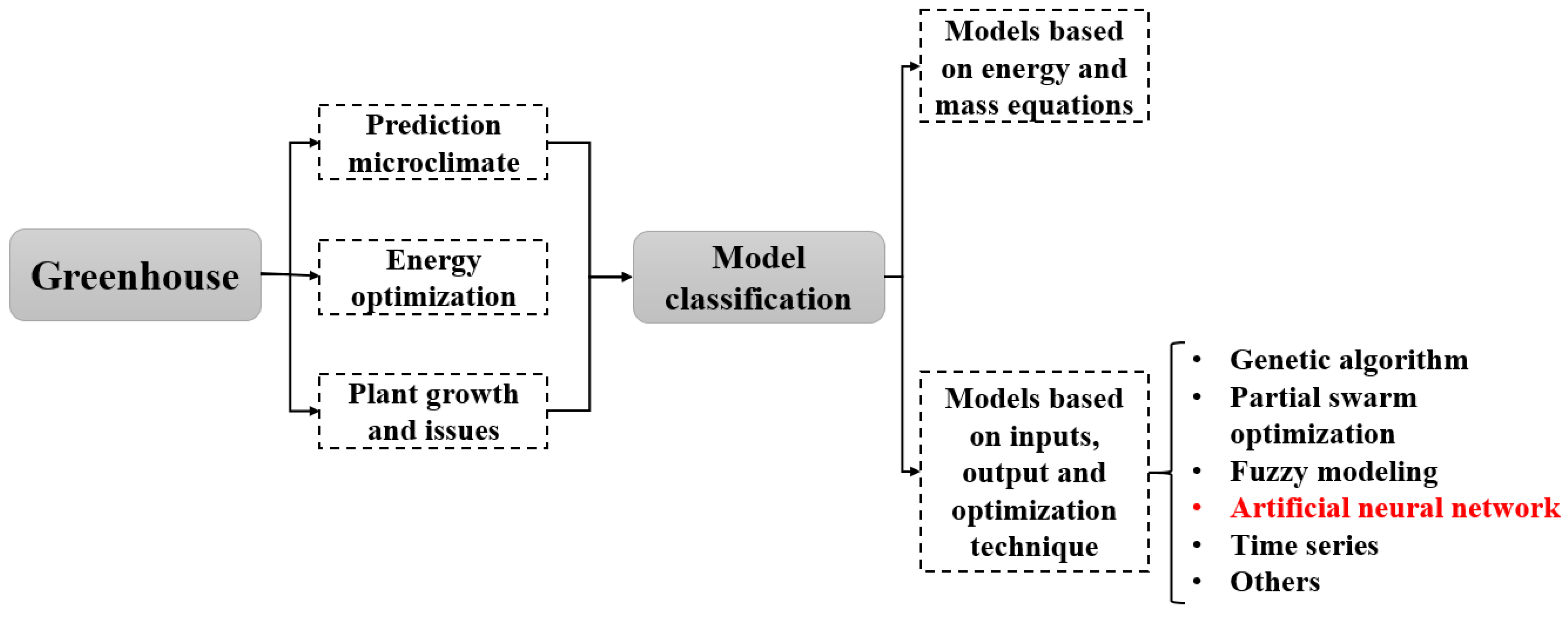
In conclusion, AI and ML techniques have become essential in accurately predicting greenhouse microclimate parameters. Accurate predictions can help optimize crop yield and quality while reducing energy consumption and environmental impact. Figure 1 describes the modeling approaches used in greenhouse control and management. Further research can explore ways to optimize these models for reducing initial costs and energy consumption while minimizing the environmental impact of greenhouse production.

Although ML methods have shown promising results in predicting greenhouse microclimate parameters, there are still some challenges that need to be addressed. One of the main challenges is the availability of high-quality data and the robustness of the models. ML models require a large amount of high-quality data to train and validate the models, but collecting and preprocessing data from greenhouse environments is often time-consuming and challenging. Another challenge is the interpretability of the ML models, which are often considered black boxes, making it difficult to understand how the models make predictions. Therefore, developing interpretable ML models that can provide insights into the underlying relationships between microclimate parameters and crop growth is essential [23,29].

To ensure reliable and accurate predictions in smart greenhouses, ANN models must be optimized for robustness across a range of environmental conditions and input variables. Recent studies have reviewed the use of AI for predicting various environmental and other variables in greenhouses, as summarized in

Table 1. Application of Artificial Intelligence (AI) in greenhouse modeling.

References	Subject	Statistical Indexes
[30]	Model predictive control via output feedback Neural Network for improved multi-window greenhouse ventilation control	RMSE value was 2.450 °C
[31]	Deep-learning-based prediction on greenhouse crop yield	RMSEs (gm−2) for 3 dataset was: 10.450, 6.760 and 7.400, respectively
[32]	Energy utilization assessment of a semi-closed greenhouse using data-driven model predictive control	RMSE value for MPC method was 0.330 °C and 0.360 °C for winter and summer simulation, respectively
[33]	Machine learning algorithms to assess the thermal behavior of a Moroccan agriculture greenhouse	R2 was 0.940 with 5-fold cross validation method
[20]	Forecasting air temperature on edge devices with embedded AI	RMSE was 0.289–0.402 °C and MAPE reported 0.87–1.04%
[34]	The use of Artificial Neural Networks for forecasting of air temperature indoor a heated foil tunnel	RMSE value reported: 3.700 °C
[13]	Neural Network model for greenhouse microclimate predictions	MAE, RMSE, and R2 were calculated to equal 0.218 K, 0.271 K, and 0.999 for temperature, and to 0.339%, 0.481%, and 0.999 for relative humidity
[35]	Evaluation of CFD and machine learning methods on predicting greenhouse microclimate parameters with the assessment of seasonality impact on machine learning performance	R > 0.980 and nRMSE < 9%
[36]	Data-driven robust model predictive control for greenhouse temperature control and energy utilization assessment	RMSE was 0.320 °C and 0.600 °C for a two-day simulation

.

Scope, Innovations and Structure

Accurately predicting greenhouse indoor climates is crucial for optimizing crop yield and quality while minimizing energy consumption. The literature reviewed in this study emphasizes the importance of investigating accurate methods for predicting the indoor climate of greenhouses. ANN models offer a more data-driven approach that can capture the non-linear relationships between input variables, such as light, humidity, and temperature. To address this issue, this research aims to investigate the potential of several AI-based models, including Artificial Neural Network with Radial Basis Function (ANN-RBF), Support Vector Machine (SVM), and Gaussian Process Regression (GPR) to estimate the indoor air temperature of an even-span polycarbonate greenhouse. The methodology employed in this study is outlined in Section 2 of the paper, which includes the study area, data collection process, and the AI methods used to predict the indoor climate of the experimental greenhouse. Section 3 reports the scientific findings of the study. The results of the RBF, SVM, and GPR model analyses are presented and compared with other similar studies. The discussion section of the paper presents suggestions for using this method in future greenhouse applications, including developing a smart control system for greenhouses. This would enable the real-time monitoring and control of the indoor climate, leading to more efficient energy use and increased crop yield. In the final part of the paper, conclusions and recommendations are presented based on the results of the study. The ultimate goal of this research and its future development is to enable smart control systems of greenhouses, leading to long-term reduction in energy losses.

2. Materials and Methods

2.1. Case Study and Data Collection

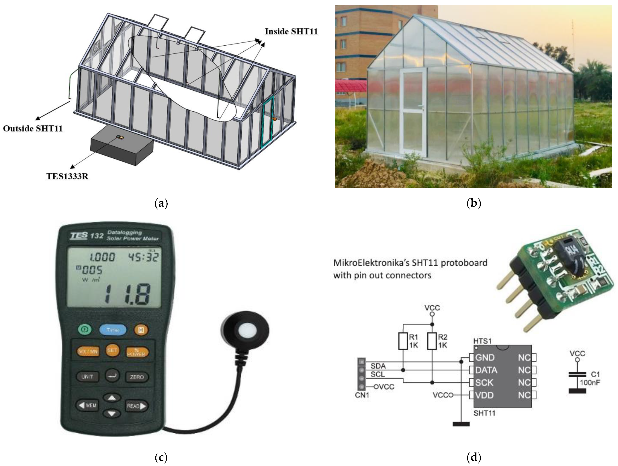
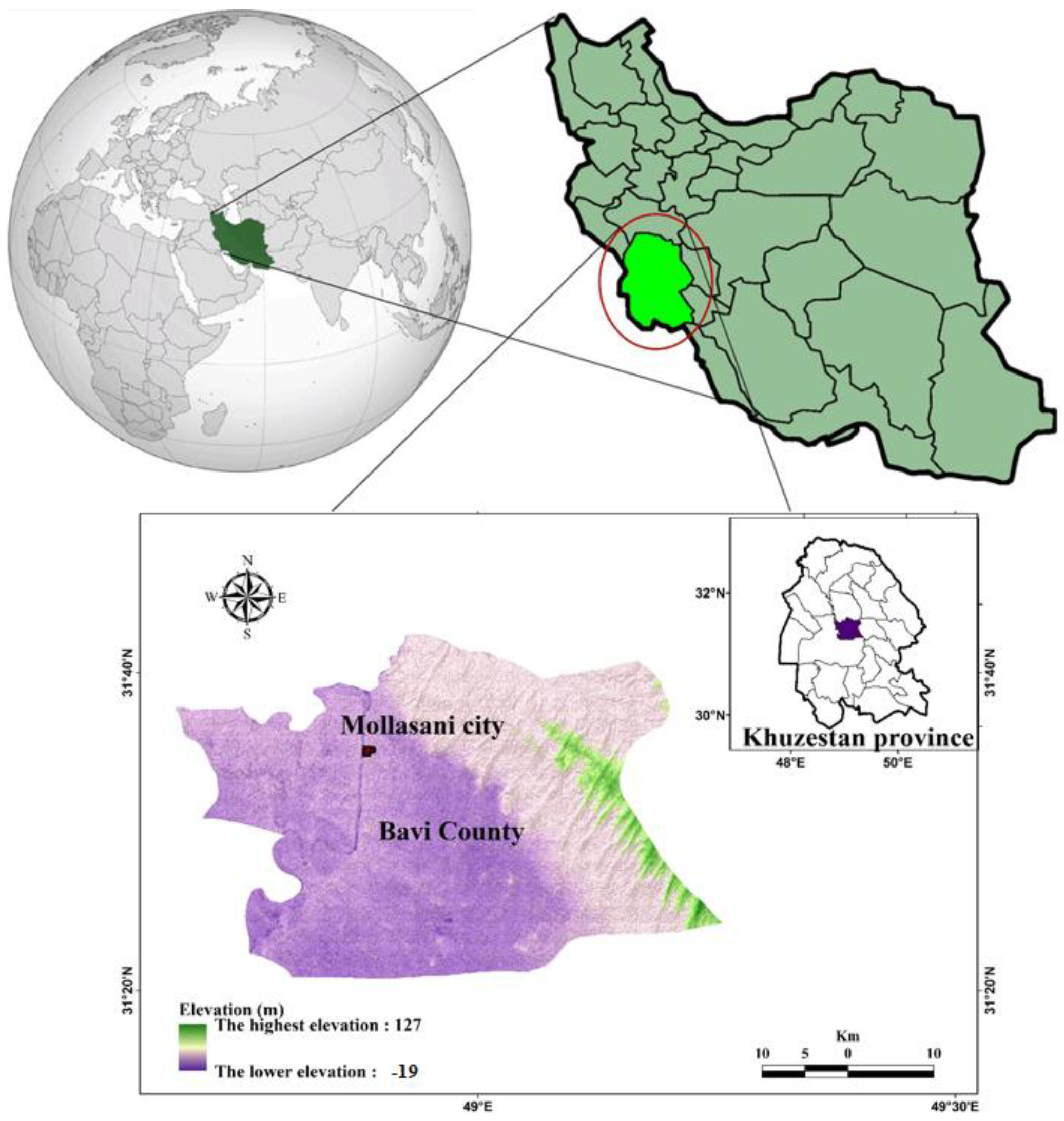
This study aimed to investigate a method for predicting the indoor air temperature in an even-span polycarbonate greenhouse at the Agricultural Sciences and Natural Resources at the University of Khuzestan, located 35 km north of Ahvaz, Iran (Latitude: 31.593; Longitude: 48.892) (Figure 2). Data were collected in August and September of 2022 from an even-span greenhouse structure with east–west orientation. It is utilized as a dryer in spring and summer and as a place for growing plants in autumn and winter, owing to the specific climatic conditions of the region. The greenhouse has a total area of 17 m², an air volume of 57 m³, and was empty of any plants. Temperature and humidity data indoor and outside the greenhouse were collected using temperature sensors (SHT 11 made by CMOS with an accuracy of ±0.4 °C and ±3% for temperature and humidity, respectively). Solar radiation data indoor the greenhouse was collected on a leveled surface using a TES1333R solar meter, which can collect radiation data in the wavelength range of 400 to 1100 nm with an accuracy of approximately 5%. Wind speed data were extracted from the data on Soda Service (https://www.soda-pro.com, accessed on 2 July 2023). An overview of the greenhouse and all the experimental devices is presented in Figure 3. For the purposes of this research, it was assumed that the greenhouse was fully enclosed and that all windows were closed during data collection. Also, the data were collected with a 5 min interval for 10 days in September–October 2022.

2.2. Radial Basis Function (RBF) Model

The ANN model is a popular prediction method comprising a minimum of three layers. The first layer, known as the input layer, has a size that is equivalent to the number of inputs in the model. In this approach, each input has an associated weight. The hidden layer comprises multiple neurons that enhance the performance of the ANN model by ensuring a sufficient number of neurons are present in this layer. The number of neurons in the output layer is equivalent to the network output. As the objective of this study is to forecast greenhouse temperatures, the output layer is configured to have just one neuron [26]. On the other hand, in the RBF method, each neuron in the hidden layer operates based on a nonlinear activation function. During the training phase of the RBF neural network, the bias factor is utilized to converge the network and achieve the global minimum [22].

To identify the most suitable network structure, the range of the spread parameter was varied from 0.1 to 1.00 in this study.

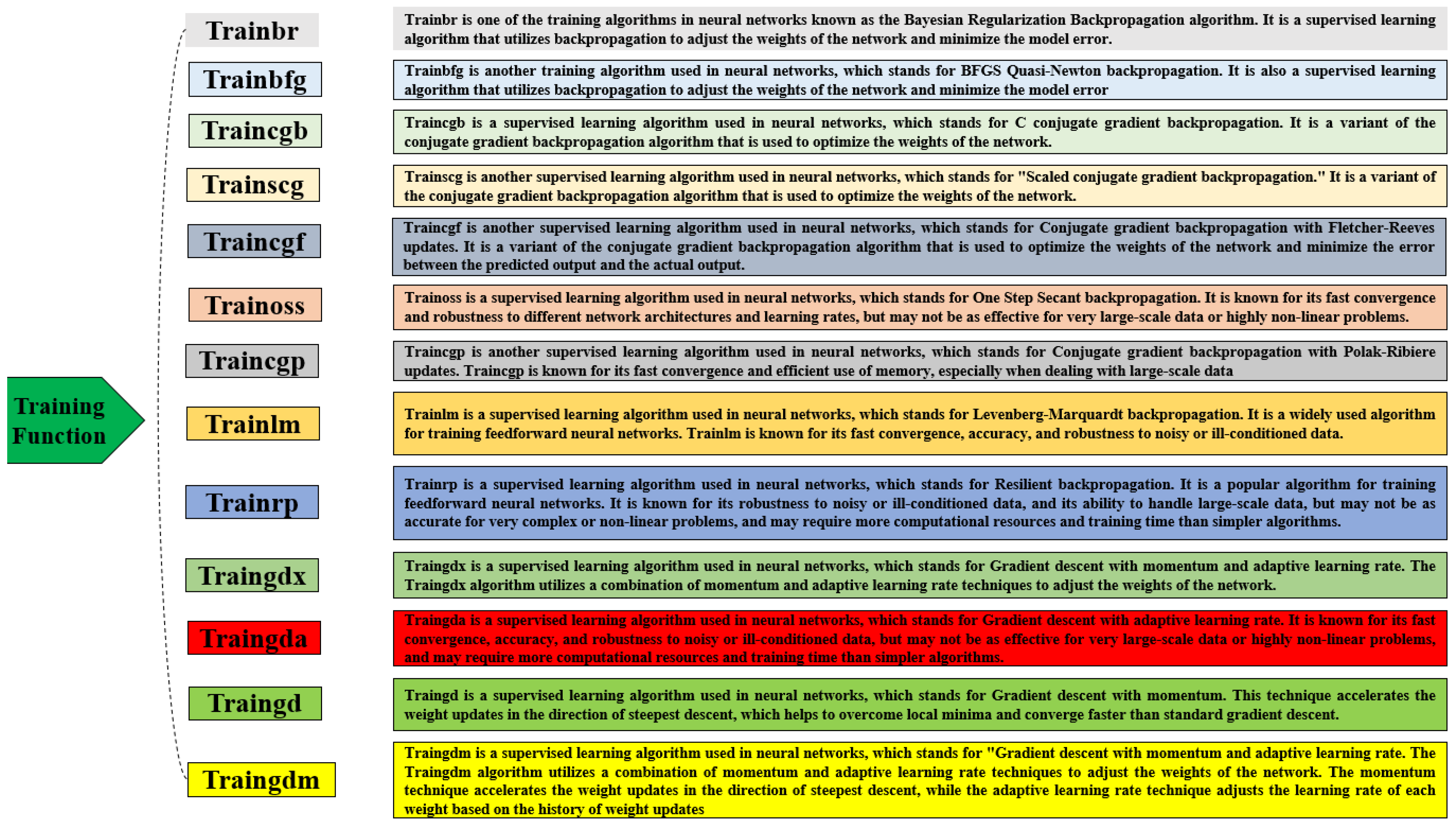
Several approaches exist for training a network and adjusting weights to minimize the error in the RBF model. Among these methods, the backpropagation algorithm of errors is one of the most commonly employed techniques, as noted by Bolandnazar et al. [26]. In this study, thirteen training functions were employed to train the models using the backpropagation training algorithms, as illustrated in Figure 4.

In the ANN model, it is feasible to approximate any optimal continuous function by incorporating a hidden layer with a sufficient number of neurons, as suggested by Rohani et al. [22]. Accordingly, a single hidden layer was employed in this study to develop the RBF model. To estimate the greenhouse temperature, the performance of the RBF method was evaluated by adjusting the number of neurons in the hidden layer from 3 to 35, and the optimal configuration was selected. Previous research has shown that linear transfer functions in the output layer of the neural network method can approximate complex functions effectively [6]. So, linear transfer functions for the RBF method were implemented in the output layer in this study.

2.3. Support Vector Machine (SVM)

The SVM model acts as a proper computational method because the SVM method can solve the quadratic optimization problems. The basic idea behind an SVM is to find a hyperplane in a high-dimensional space that separates the data into different classes [26]. The hyperplane is chosen so as to maximize the margin between the classes, which is defined as the distance between the hyperplane and the closest data points from each class [19]. During the training phase, the SVM algorithm learns the optimal hyperplane by finding the set of parameters that minimizes the classification error on the training data. Once the hyperplane has been learned, it can be used to predict the class label of new, unseen data points [19]. To make a prediction using an SVM model, the algorithm takes the input data and maps it into the high-dimensional feature space used during training. It then applies the learned hyperplane to the transformed data to obtain a score or decision function. The sign of the decision function indicates the predicted class label: if the decision function is positive, the data point is classified into one class, and if it is negative, it is classified into the other class. The magnitude of the decision function also provides a measure of confidence in the prediction [22].

2.4. Gaussian Process Regression (GPR) Model

Gaussian Process Regression (GPR) is a powerful statistical modeling technique that is used to model complex data distributions and make predictions based on noisy or incomplete data. It is a non-parametric approach that assumes a prior probability distribution over the possible functions that could fit the data and updates this distribution as new data are observed [37]. In GPR, the prior distribution over functions is represented by a Gaussian process, which is a collection of random variables that are jointly Gaussian distributed. The covariance between any two points in the input space determines the similarity between those points and is used to make predictions about the output variable. The hyper parameters of the Gaussian process, such as the length scale and amplitude, control the smoothness and variability of the functions in the prior distribution [38]. The posterior distribution over functions is obtained by conditioning on the observed data and is also a Gaussian process with updated mean and covariance functions. This allows for the computation of predictive distributions, and uncertainty estimates for new input points. GPR has many advantages over other regression techniques, such as its ability to model nonlinear and non-parametric relationships, flexibility in choosing the covariance function, and ability to provide uncertainty estimates for predictions [21]. It has been successfully applied in many fields, including engineering, finance, and biology. However, GPR can be computationally intensive and may require a careful choice of hyper parameters and covariance functions. It also assumes that the data are stationary and does not account for non-Gaussian noise in the data [21].

The GPR model aims to learn from training data and perform well in extrapolating the output distribution to unseen input locations [39]. In this context, the noise in the output model accounts for the uncertainty introduced by factors other than the input variable x, such as observational errors. This study assumes that the noise is additive, has a zero mean, is stationary, and tends to be randomly dispersed [22]:

$$y=f(x)+\epsilon \mathrm{and} \epsilon \simeq N(0,{\mathrm{s}}_{\mathrm{noise}}^2)$$

(1)

where ${\mathrm{s}}_{\mathrm{noise}}^2$ is the variance of the noise. The Gaussian prior assumption enables the function to be interpreted through the mean m(x) and covariance functions. As suggested by the existing literature, the shape of the mean function is only significant in unobserved regions and is often assumed to be zero [21].

2.5. Performance Evaluation Criteria

Various performance metrics were employed in this study to evaluate the effectiveness of the RBF, SVM, and GPR models in predicting the indoor temperature in a greenhouse. These metrics include the Mean Absolute Percentage Error (MAPE), Root Mean Square Error (RMSE), Total Sum of Squared Error (TSSE), and Efficiency Factor (EF). In this study, the model exhibiting the highest accuracy is determined by achieving the lowest MAPE, RMSE, and TSSE values, and the highest EF value [22].

3. Results and Discussion

This study aimed to predict the indoor air temperature of an even-span polycarbonate greenhouse using three different machine learning models, namely RBF, SVM, and GPR. The dataset comprised observations from an even-span polycarbonate greenhouse, with four factors used as inputs: Outside Solar Radiation (I_out) (Wm⁻²), Outside Air Temperature (T_out) (°C), Outside Air Humidity (Rh_out) (%), and Outside Wind Speed (W_out).

3.1. Climate Condition of the Study Area

Figure 5 shows the climate variations in the studied area, which can impact crop growth and productivity. The summer months in this region are characterized by high temperatures that can exceed 50 °C, which can limit the growth of some crops when grown outside. While greenhouse cultivation can provide optimal conditions for plant growth, it also requires energy-intensive cooling systems to maintain suitable temperatures for most of the time in the study area. Additionally, the high levels of solar radiation in the region can be beneficial for plant growth; however, they can also lead to heat stress and damage to crops if not adequately managed. The low wind speeds in this region can be advantageous for greenhouse cultivation, as they create a stable environment for plant growth and reduce the risk of physical damage to the greenhouse structure. However, high humidity levels during the summer and winter months can increase the spread of plant diseases, which can be a significant challenge for greenhouse cultivation.

3.2. Selection of the Best Perform Models

This section presents the performance of several models in predicting the indoor air temperature of the greenhouse, with the best-performing model selected.

Table 2. Greenhouse temperature prediction by RBF, SVM, and GPR models.

Model	Train				Test				Total
	RMSE	MAPE	TSSE	EF	RMSE	MAPE	TSSE	EF	RMSE	MAPE	TSSE	EF
RBF	0.80	1.19	367	1.00	0.91	1.30	108	0.99	0.82	1.21	474	1.00
SVM	1.97	3.13	2207	0.97	2.13	3.70	596	0.97	2.00	3.24	2803	0.97
GPR	1.29	1.93	949	0.99	2.19	4.12	626	0.97	1.50	2.34	1575	0.98

shows the statistical metrics employed to assess the accuracy of the models in the training, test, and overall phases, which include MAPE, RMSE, TSSE, and EF. The results indicate that the RBF model outperformed the other models in predicting the greenhouse indoor air temperature, achieving a MAPE index ranging from 1.19 to 1.30%. The RBF model showed lower MAPE values in the training and test phases than the GPR and SVM models. On the other hand, the GPR model also demonstrated good accuracy for predicting the indoor air temperature, while the SVM model did not perform well in this study. Based on the results, the RBF model was selected for further analysis and development in the remaining parts of the study. It should be noted that the use of this model is crucial for accurately predicting the greenhouse indoor air temperature and ensuring the optimal growth of crops.

Ali and Hassanein [40], developed a Recurrent Neural Network (RNN) model with long short-term memory to predict environmental parameters in greenhouses, specifically for tomato production. The model exhibited high accuracy and demonstrated its ability to predict future temperatures, achieving an RMSE value of 0.7. Similarly, Petrakis and Kavga [13], implemented neural network models to forecast microclimates in greenhouses located in Greece. The results indicated maximum errors of 0.88 K and 2.84% for modeled temperature and relative humidity, respectively, while the coefficients of determination were both 0.99 for these parameters.

3.3. Input Parameters Optimization

In this step, a sensitivity analysis was performed to develop and improve the selected RBF model by considering the effects of the outside environment’s temperature, humidity, radiation, and wind speed on the input data. The sensitivity analysis can provide valuable insights into the behavior of the system and help identify the critical variables that affect the model’s accuracy. By incorporating the effects of these variables into the model, the accuracy of the predictions can be enhanced, leading to improved performance and efficiency of predictions. The variables were evaluated individually and then as a group to determine their impact on the accuracy of the RBF model.

Table 3. Sensitivity analysis for prediction the indoor air temperature of greenhouse.

Variables	Train				Test				Total
	EF	TSSE	MAPE	RMSE	EF	TSSE	MAPE	RMSE	EF	TSSE	MAPE	RMSE
All except Rhout	1.48	2.08	1236.62	0.99	1.53	2.41	308.3	0.99	1.49	2.14	1545.01	0.99
All except Tout	1.67	2.27	1590.1	0.98	1.52	2.41	300.94	0.99	1.65	2.27	1891.04	0.98
All except Iout	2.07	3.05	2419.2	0.97	1.91	2.83	480.31	0.98	2.04	3.01	2899.51	0.97
All except Wout	0.84	1.22	398.44	1	0.96	1.51	120.42	0.99	0.86	1.27	518.86	0.99
All data	0.8	1.19	366.52	1	0.91	1.3	107.56	0.99	0.82	1.21	474.07	1

presents the results of the sensitivity analysis.

The findings reveal that including all input variables as datasets for RBF model training leads to greater accuracy. This finding suggests that all the input variables play a critical role in predicting the greenhouse indoor air temperature and that the RBF model’s performance can be improved by considering all the variables simultaneously.

According to the sensitivity analysis results presented in Table 3, all four input variables, namely outside temperature, humidity, radiation, and wind speed, will be utilized as the primary dataset to train the RBF model in the subsequent steps. The inclusion of these variables is expected to result in more accurate predictions of the indoor air temperature in the greenhouse. Based on the outcomes displayed in Table 2, the combination of outside temperature, humidity, solar radiation, and wind speed was selected as the input dataset for the RBF model in the subsequent steps of the study. This decision was based on the sensitivity analysis results, indicating that considering all four variables simultaneously can enhance the accuracy of the RBF model in forecasting the indoor air temperature of the greenhouse.

3.4. Optimization of Dataset Sizes

The size of the dataset used to train the RBF network can have a significant impact on the accuracy and performance of the model. Generally, larger datasets lead to more accurate predictions and can help avoid overfitting, which occurs when the model memorizes the training data and performs poorly on new data. However, using a large dataset can also increase the computational complexity and training time of the model, which can be a limiting factor in some applications. In contrast, using a small dataset can result in under-fitting, where the model fails to capture the complex relationships between the input and output variables.

To determine the optimal dataset size for training the RBF network, a sensitivity analysis can be performed by training the model with different dataset sizes and evaluating its performance using various statistical metrics. This approach can help identify the minimum dataset size required for accurate predictions, while also avoiding overfitting and excessive computational complexity.

This section evaluates the impact of dataset size on the accuracy of the RBF model by varying the size of the dataset and analyzing the resulting changes in the model’s accuracy (

Table 4. Predicting greenhouse indoor air temperature using all variables as inputs with varying data sizes.

The Share of Dataset	Train				Test				Total
	EF	TSSE	MAPE	RMSE	EF	TSSE	MAPE	RMSE	EF	TSSE	MAPE	RMSE
80	0.81	1.28	364	1	1.02	1.55	147	0.99	0.86	1.33	511	1
70	0.92	1.31	415	0.99	0.85	1.29	152	0.99	0.9	1.3	568	0.99
60	1.16	1.39	565	0.99	1.13	1.45	339	0.99	1.15	1.59	920	0.99
50	1.05	1.39	383	0.99	0.99	1.45	339	0.99	1.02	1.42	722	0.99

).

The results indicate that the optimal dataset size for training the RBF model to predict the indoor air temperature in the greenhouse is 80% of the total dataset. This implies that the model achieves the highest accuracy when trained with 80% of the total dataset. The MAPE index for predicting the indoor air temperature in the entire phases was 1.33%, demonstrating that the RBF model can accurately predict the output. However, in the standard mode, the best results may not always be achieved when 60% of the total data are used for network training, as observed in this study. To ensure the highest accuracy of the RBF model, the dataset size for training the model was fixed at 80% in the subsequent analyses. This study emphasizes the importance of selecting the optimal dataset size to achieve the best results and avoid overfitting or under-fitting.

3.5. Selection of Best Training Algorithm for RBF Model

The selection of the best training algorithm for the RBF neural network model can have a significant impact on the accuracy and performance. Different training algorithms can vary in their convergence speed, computational complexity, and ability to avoid overfitting. One commonly used training algorithm for RBF neural networks is the backpropagation algorithm, which involves iteratively adjusting the weights and biases of the network to minimize the error between the predicted and actual outputs. While the backpropagation algorithm can be effective in training RBF models, it may also suffer from slow convergence and the risk of getting trapped in local minima. Other training algorithms, such as the Levenberg–Marquardt algorithm, can offer faster convergence and better generalization performance by adjusting the learning rate based on the curvature of the error surface. The Quasi–Newton algorithm can also be effective in training RBF models by approximating the second derivative of the error function and adjusting the weights and biases accordingly.

In this study, the performance of 13 different training algorithms for the RBF neural network model was evaluated and compared (

Table 5. Optimizing training algorithm selection for predicting greenhouse indoor air temperature using statistical indexes in train, test, and total phases.

Training Algorithm	Train				Test				Total
	RMSE	MAPE	TSSE	EF	RMSE	MAPE	TSSE	EF	RMSE	MAPE	TSSE	EF
trainlm	0.80	1.19	367	1.00	0.91	1.30	108	0.99	0.82	1.21	474	1.00
trainbr	0.84	1.31	401	1.00	1.08	1.62	152	0.99	0.89	1.37	552	0.99
trainbfg	1.07	1.55	646	0.99	1.13	1.72	168	0.99	1.08	1.59	815	0.99
traincgb	1.30	1.82	963	0.99	1.12	1.77	164	0.99	1.27	1.81	1127	0.99
traincgf	1.34	1.86	1025	0.99	1.22	1.94	194	0.99	1.32	1.87	1219	0.99
traincgp	1.32	1.91	988	0.99	1.36	2.21	243	0.99	1.33	1.97	1231	0.99
trainrp	1.34	1.98	1019	0.99	1.34	2.16	235	0.99	1.34	2.01	1254	0.99
trainoss	1.41	2.00	1126	0.99	1.39	2.12	252	0.99	1.41	2.03	1378	0.99
traingdx	1.54	2.22	1348	0.98	1.34	2.24	236	0.99	1.51	2.22	1584	0.98
trainscg	1.62	2.41	1484	0.98	1.39	2.50	252	0.99	1.58	2.43	1736	0.98
traingda	1.71	2.47	1658	0.98	1.41	2.48	259	0.99	1.66	2.47	1917	0.98
traingdm	2.63	4.06	3921	0.95	1.89	3.28	470	0.98	2.51	3.91	4392	0.80
traingd	5.50	10.28	17151	0.79	5.42	11.07	3851	0.82	5.49	10.43	21003	0.80

). The results indicate that the Levenberg–Marquardt algorithm (trainlm) achieved the lowest MAPE, RMSE, and TSSE, as well as the highest EF at the total phase, indicating superior accuracy and performance compared to the other algorithms evaluated. The Levenberg–Marquardt algorithm is a popular training algorithm for RBF neural networks due to its ability to converge more quickly than other algorithms such as the backpropagation algorithm, while also being less prone to overfitting than more complex algorithms like the Bayesian regularization algorithm. The use of the Levenberg–Marquardt algorithm in the next analysis is expected to lead to the improved accuracy and performance of the RBF neural network model for predicting greenhouse indoor air temperature, particularly when training on large datasets. Castañeda-Miranda and Castaño [41] utilized a Multi-Layer Perceptron (MLP) Artificial Neural Network (ANN) to predict greenhouse air temperature. The ANN was trained with a Levenberg–Marquardt backpropagation algorithm, with the input parameters consisted of outside air temperature and relative humidity, global solar radiation, wind speed, and indoor relative humidity. The study reported a temperature forecast with 95% confidence, achieving a coefficient of determination of 0.96 in winter and 0.95 in summer. Yue et al. [42], proposed an improved Levenberg–Marquardt Radial Basis Function Neural Network (LM-RBF) model to forecast greenhouse air temperature and humidity. Their model achieved a maximum relative error of less than 0.5%.

3.6. Optimization of Hidden Layer Neurons

The hidden layer of the RBF neural network model plays a critical role in transforming the input data into a new space that is more suitable for linearly separable analysis. Unlike linear models, the RBF model can handle nonlinear patterns in the input data by transforming them into a higher-dimensional space through the hidden layer. The number of neurons in the hidden layer is an important parameter that affects the model’s ability to capture complex relationships between the input and output variables. Cover’s theorem on the reparability of patterns suggests that nonlinear patterns in the input data can be transformed into a higher-dimensional space to make them more linearly separable. So, the number of neurons in the hidden layer should be greater than the number of input neurons to increase the dimensionality of the transformed space and improve the model’s ability to capture nonlinear relationships. Also, the optimal number of neurons in the hidden layer depends on the complexity of the input and output data, as well as the degree of nonlinearity in the relationships between them. A small number of neurons in the hidden layer can lead to under-fitting, where the RBF model is too simple and unable to capture the complex relationships between the input and output variables. On the other hand, a large number of neurons in the hidden layer can result in overfitting, where the RBF model memorizes the training data and performs poorly on new data. To determine the optimal number of neurons in the hidden layer, a sensitivity analysis can be performed by training the RBF model with different numbers of neurons and evaluating its performance using various statistical metrics. This approach can help identify the optimal number of neurons that achieves the best balance between overfitting and under-fitting and achieves the best accuracy and efficiency. This study examines the impact of the number of neurons in the hidden layer on the accuracy and performance of the RBF neural network model in predicting the indoor air temperature of the greenhouse. The number of neurons in the hidden layer was varied from 3 to 35, and the model’s performance was evaluated based on the lowest error and highest accuracy (Figure 6). The findings demonstrate that the optimal number of neurons in the hidden layer was 33. By fixing the number of neurons in the hidden layer to this value, the MAPE factor reduced to 1.3%, indicating a significant enhancement in the model’s accuracy and performance. Francik and Kurpaska [34] developed a three-layer Perceptron neural network with 10 neurons in the hidden layer, utilizing temperature, wind speed, solar radiation, and forecast time as input parameters to forecast temperature changes in a heated foil tunnel. The study achieved the lowest RMSE value (3.7 °C) for the testing dataset.

3.7. Effect of Spread Factor on the Efficiency of RBF Model

The spread factor is a crucial parameter in the RBF model that can significantly impact the efficiency and accuracy of the model. The spread factor determines the width of the RBF kernel function, which affects the degree of overlap between the RBF functions and the spatial distribution of the input data.

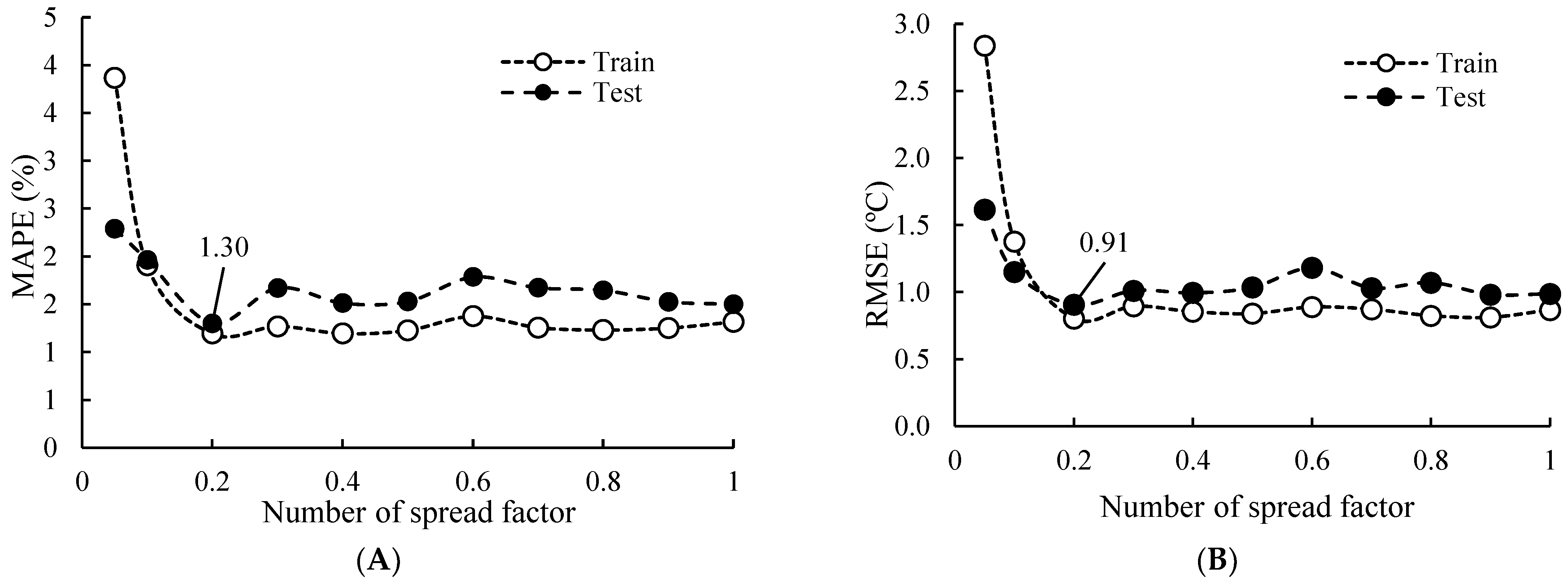
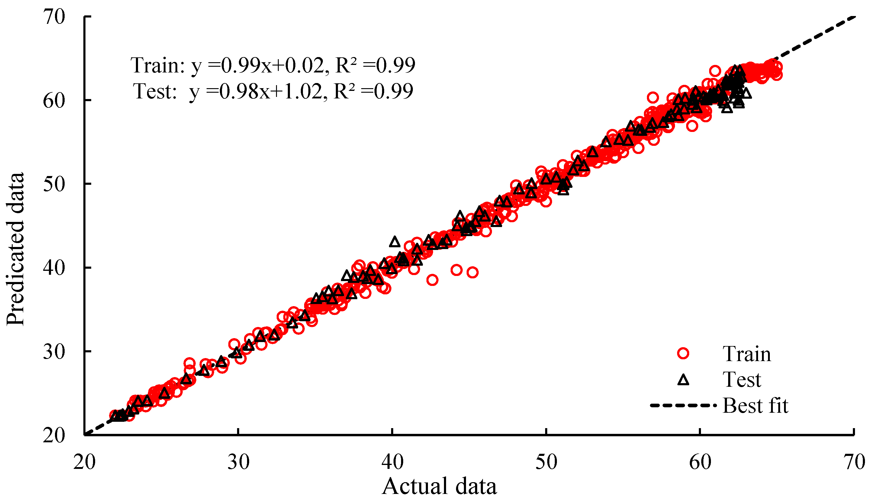
To determine the optimal spread factor for the RBF model, a sensitivity analysis can be performed by training the model with different spread factors and evaluating its performance using various statistical metrics. This approach can help identify the optimal spread factor that balances between overfitting and under-fitting and achieves the best accuracy and efficiency. In general, the optimal spread factor depends on the characteristics of the input data and the complexity of the relationships between the input and output variables. For complex and highly nonlinear systems, a smaller spread factor may be more appropriate, while simpler systems may require a larger spread factor. In this study, the spread factor was varied from 0.1 to 1, and for each value, the MAPE, RMSE, TSSE, and EF factors were computed (Figure 7). The results indicate that, by selecting 0.2 for spread factor, the accuracy can considerable increase. This finding highlights the importance of selecting an optimal spread factor to achieve the best results in RBF modeling. The MAPE and RMSE at the training and test phases are 1.30% and 0.91 °C, respectively. Figure 8 shows the distribution of actual and predicted data (45-degree line) from the RBF model. It can be concluded that the RBF model could predict the indoor air temperature of greenhouse with high accuracy and can be used for climate controlling in smart greenhouses.

In a study, a hybrid artificial neural network (ANN) was utilized to predict freshwater production in seawater greenhouses [43]. The study demonstrated that the ANN method is highly accurate, with negligible differences between actual and predicted data. In another study, machine learning algorithms were employed to predict indoor air temperature in Moroccan agriculture greenhouses [33]. The results showed that all predictive models performed well, with an R² value greater than 0.9.

Table 6. Comparing the performance of RBF model with actual data at all phases of modeling.

Phases	Data	Average	Variance	Standard Deviation	Minimum	Maximum	Kurtosis	Skewness	Sum
Train	Actual	49.51	145.98	12.08	22.02	65.00	2.45	−0.77	28073.90
	Predicted	49.50	146.40	12.10	22.33	64.25	2.43	−0.77	28065.41
Predicted values = 0.99 × Actual values + (0.02) R2 = 0.99
Test	Actual	49.32	161.77	12.72	22.00	63.00	2.24	−0.67	6460.87
	Predicted	49.38	156.29	12.50	22.33	63.58	2.33	−0.71	6469.36
Predicted values = 0.98 × Actual values + (0.1.02) R2 = 0.99
Total	Actual	49.48	148.72	12.20	22.00	65.00	2.41	−0.75	34534.77
	Predicted	49.48	148.04	12.17	22.33	64.25	2.41	−0.76	34534.77

shows the statistical properties of the data utilized in the training, test, and overall stages of the selected RBF structure for predicting the indoor air temperature in the greenhouse. The outcomes demonstrate that the differences between the minimum, maximum, variance, and skewness of the actual and predicted data are negligible, which is insignificant for practical purposes.

The best model results are obtained when the linear relationship between the actual and predicted values has the highest coefficient of determination, the narrowest width from the origin, and a slope close to one. In this study, the RBF model exhibited a strong correlation coefficient in the training and testing phases, with regression relationships having the smallest width from the origin and a slope close to one. Hence, this model is considered the best for prediction. To further evaluate the RBF model, various statistical tests were conducted in this study. The tests analyzed the average, variance, and statistical distribution of the actual and predicted values by the RBF model in different stages of training, testing, and overall. The null hypothesis for each test is the equality of mean, variance, and statistical distribution of both data series:

$$\left\{\begin{array}{l}{H}_0:{\overline{y}}_a={\overline{y}}_p\\ H_1:{\overline{y}}_a\ne {\overline{y}}_p\end{array}\right. \mathrm{and} \left\{\begin{array}{l}{H}_0:{\sigma }_{ya}^2={\sigma }_{yp}^2\\ H_1:{\sigma }_{ya}^2\ne {\sigma }_{yp}^2\end{array}\right. \mathrm{and} \left\{\begin{array}{l}{H}_0:d_a=d_p\\ H_1:d_a\ne d_p\end{array}\right.$$

(2)

At a significance level of 95%, each hypothesis was tested using the p-value parameter. If the calculated p-value for each stage exceeds 0.05, the null hypothesis cannot be rejected. To compare the mean, variance, and statistical distribution, t-tests, F-tests, and Kolmogorov–Smirnov tests were employed.

Table 7. Performance of optimized RBF model for greenhouse indoor air temperature prediction.

Phases	Types of Statistical Analysis			Final Statistical Indexes of RBF Model
	Average	Variance	Distribution	RMSE	MAPE	TSSE	EF
Training	0.98	0.97	0.82	0.80	1.19	366.52	1.00
Test	0.97	0.84	0.52	0.91	1.30	107.56	0.99
Total	1.00	0.95	0.87	0.82	1.21	474.07	1.00

shows the p-values computed for all three stages (training, test, and overall).

The results demonstrate that the mean, variance, and statistical distribution values of the data obtained from the RBF model exhibit no significant difference from the actual values, indicating that this model can be utilized with high reliability.

4. Conclusions

Machine learning (ML) techniques have become increasingly important in modeling complex systems. ML enables more accurate and reliable predictions by leveraging large datasets and capturing complex relationships between input variables and output targets. In the context of predicting indoor air temperature, ML models can account for various factors, such as outdoor temperature, humidity, solar radiation, and occupant behavior, resulting in more comprehensive and holistic predictions. These predictions can be beneficial for optimizing energy consumption, improving indoor comfort and air quality, and reducing greenhouse gas emissions. Furthermore, ML models can adapt to changing conditions and learn from experience, making them ideal for predicting indoor air temperature in dynamic environments.

The primary objective of this study was to develop accurate ML models for predicting indoor air temperature in an even-span polycarbonate greenhouse using RBF, SVM, and GPR models. The results of the study are presented as follows:

• The comparison of the three models revealed that the RBF model was the most effective in accurately predicting greenhouse temperature. The RBF model achieved the lowest RMSE values during the training and test phases, at 0.80 °C and 0.91 °C, respectively.
• The evaluation of the RBF model’s performance showed that the dataset size, value of spared factor, number of neurons in the hidden layer, and type of training algorithm significantly impacted the output.
• Accurate temperature prediction is crucial for achieving the goal of smart greenhouse operation, and the high accuracy and reliability of the RBF model make it a valuable tool for optimizing greenhouse management, improving time management, and increasing crop yields. The performance results of this study indicate that integrating artificial neural network (ANN) models into the control system can assist farmers in building smart greenhouses.

References

1. Amini, S.; Taki, M.; Rohani, A. Applied improved RBF neural network model for predicting the broiler output energies. Appl. Soft Comput. J. 2020, 87, 106006. [Google Scholar] [CrossRef]
2. Azizpanah, A.; Fathi, R.; Taki, M. Eco-energy and environmental evaluation of cantaloupe production by life cycle assessment method. Environ. Sci. Pollut. Res. 2022, 30, 1854–1870. [Google Scholar] [CrossRef] [PubMed]
3. Taki, M.; Ajabshirchi, Y.; Ranjbar, S.F.; Rohani, A.; Matloobi, M. Modeling and experimental validation of heat transfer and energy consumption in an innovative greenhouse structure. Inf. Process. Agric. 2016, 3, 157–174. [Google Scholar] [CrossRef] [Green Version]
4. Daliran, A.; Taki, M.; Marzban, A.; Rahnama, M.; Farhadi, R. Experimental evaluation and modeling the mass and temperature of dried mint in greenhouse solar dryer; Application of machine learning method. Case Stud. Therm. Eng. 2023, 47, 103048. [Google Scholar] [CrossRef]
5. Parajuli, S.; Narayan, T.; Gorjian, S.; Vithanage, M.; Raj Paudel, S. Assessment of potential renewable energy alternatives for a typical greenhouse aquaponics in Himalayan Region of Nepal. Appl. Energy 2023, 344, 121270. [Google Scholar] [CrossRef]
6. Taki, M.; Ajabshirchi, Y.; Ranjbar, S.F.; Rohani, A.; Matloobi, M. Heat transfer and MLP neural network models to predict indoor environment variables and energy lost in a semi-solar greenhouse. Energy Build. 2016, 110, 314–329. [Google Scholar] [CrossRef]
7. Figueiroa, V.; Torres, J.P.N. Simulation of a Small Smart Greenhouse. Designs 2022, 6, 106. [Google Scholar] [CrossRef]
8. Cafuta, D.; Dodig, I.; Cesar, I.; Kramberger, T. Developing a Modern Greenhouse Scientific Research Facility—A Case Study. Sensors 2021, 21, 2575. [Google Scholar] [CrossRef]
9. Singh, R.K.; Rahmani, M.H.; Weyn, M.; Berkvens, R. Joint Communication and Sensing: A Proof of Concept and Datasets for Greenhouse Monitoring Using LoRaWAN. Sensors 2022, 22, 1326. [Google Scholar] [CrossRef]
10. Rasheed, A.; Kwak, C.S.; Kim, H.T.; Lee, H.W. Building Energy an Simulation Model for Analyzing Energy Saving Options of Multi-Span Greenhouses. Appl. Sci. 2020, 10, 6884. [Google Scholar] [CrossRef]
11. Ahamed, M.S.; Guo, H.; Tanino, K. Energy saving techniques for reducing the heating cost of conventional greenhouses. Biosyst. Eng. 2019, 178, 9–23. [Google Scholar] [CrossRef]
12. Cao, Q.; Wu, Y.; Yang, J.; Yin, J. Greenhouse Temperature Prediction Based on Time-Series Features and LightGBM. Appl. Sci. 2023, 13, 1610. [Google Scholar] [CrossRef]
13. Petrakis, T.; Kavga, A.; Thomopoulos, V.; Argiriou, A.A. Neural Network Model for Greenhouse Microclimate Predictions. Agriculture 2022, 12, 780. [Google Scholar] [CrossRef]
14. Zhang, C.; Liu, H.; Wang, C.; Zong, Z.; Wang, H.; Zhao, X.; Wang, S.; Li, Y. Testing and Analysis on the Spatial and Temporal Distribution of Light Intensity and CO2 Concentration in Solar Greenhouse. Sustainability 2023, 15, 7001. [Google Scholar] [CrossRef]
15. Aamir, M.; Bhatti, M.A.; Bazai, S.U.; Marjan, S.; Mirza, A.M.; Wahid, A.; Hasnain, A.; Bhatti, U.A. Predicting the Environmental Change of Carbon Emission Patterns in South Asia: A Deep Learning Approach Using BiLSTM. Atmosphere 2022, 13, 2011. [Google Scholar] [CrossRef]
16. Faniyi, B.; Luo, Z.A. Physics-Based Modelling and Control of Greenhouse System Air Temperature Aided by IoT Technology. Energies 2023, 16, 2708. [Google Scholar] [CrossRef]
17. Chen, T.-H.; Lee, M.-H.; Hsia, I.-W.; Hsu, C.-H.; Yao, M.-H.; Chang, F.-J. Develop a Smart Microclimate Control System for Greenhouses through System Dynamics and Machine Learning Techniques. Water 2022, 14, 3941. [Google Scholar] [CrossRef]
18. Bazgaou, A.; Fatnassi, H.; Bouharroud, R.; Tiskatine, R.; Wifaya, A.; Demrati, H.; Bammou, L.; Aharoune, A.; Bouirden, L. CFD Modeling of the Microclimate in a Greenhouse Using a Rock Bed Thermal Storage Heating System. Horticulturae 2023, 9, 183. [Google Scholar] [CrossRef]
19. Taki, M.; Abdanan Mehdizadeh, S.; Rohani, A.; Rahnama, M.; Rahmati-Joneidabad, M. Applied machine learning in greenhouse simulation; new application and analysis. Inf. Process. Agric. 2018, 5, 253–268. [Google Scholar] [CrossRef]
20. Codeluppi, G.; Davoli, L.; Ferrari, G. Forecasting Air Temperature on Edge Devices with Embedded AI. Sensors 2021, 21, 3973. [Google Scholar] [CrossRef]
21. Taki, M.; Rohani, A.; Sohelifard, F.; Abdeshahi, A. Assessment of energy consumption and modeling of output energy for wheat production by neural network (MLP and RBF) and Gaussian process regression (GPR) models. J. Clean. Prod. 2018, 172, 3028–3041. [Google Scholar] [CrossRef]
22. Rohani, A.; Taki, M.; Abdollahpour, Z. A novel soft computing model (Gaussian process regression with K-fold cross validation) for daily and monthly solar radiation forecasting (Part: I). Renew. Energy 2018, 115, 411–422. [Google Scholar] [CrossRef]
23. Jung, D.-H.; Lee, T.S.; Kim, K.; Park, S.H. A Deep Learning Model to Predict Evapotranspiration and Relative Humidity for Moisture Control in Tomato Greenhouses. Agronomy 2022, 12, 2169. [Google Scholar] [CrossRef]
24. González-Vidal, A.; Mendoza-Bernal, J.; Ramallo, A.P.; Zamora, M.Á.; Martínez, V.; Skarmeta, A.F. Smart Operation of Climatic Systems in a Greenhouse. Agriculture 2022, 12, 1729. [Google Scholar] [CrossRef]
25. Liu, R.; Yuan, S.; Han, L. Evaluation and Analysis on the Temperature Prediction Model for Bailing Mushroom in Jizhou, Tianjin. Agriculture 2022, 12, 2044. [Google Scholar] [CrossRef]
26. Bolandnazar, E.; Rohani, A.; Taki, M. Energy consumption forecasting in agriculture by artificial intelligence and mathematical models. Energy Sources Part A Recover. Util. Environ. Eff. 2020, 42, 1618–1632. [Google Scholar] [CrossRef]
27. Jin, X.-B.; Zheng, W.-Z.; Kong, J.-L.; Wang, X.-Y.; Zuo, M.; Zhang, Q.-C.; Lin, S. Deep-Learning Temporal Predictor via Bidirectional Self-Attentive Encoder–Decoder Framework for IOT-Based Environmental Sensing in Intelligent Greenhouse. Agriculture 2021, 11, 802. [Google Scholar] [CrossRef]
28. Ojo, M.O.; Zahid, A. Deep Learning in Controlled Environment Agriculture: A Review of Recent Advancements, Challenges and Prospects. Sensors 2022, 22, 7965. [Google Scholar] [CrossRef]
29. Escamilla-García, A.; Soto-Zarazúa, G.M.; Toledano-Ayala, M.; Rivas-Araiza, E.; Gastélum-Barrios, A. Applications of Artificial Neural Networks in Greenhouse Technology and Overview for Smart Agriculture Development. Appl. Sci. 2020, 10, 3835. [Google Scholar] [CrossRef]
30. Jung, D.-H.; Kim, H.-J.; Kim, J.Y.; Lee, T.S.; Park, S.H. Model Predictive Control via Output Feedback Neural Network for Improved Multi-Window Greenhouse Ventilation Control. Sensors 2020, 20, 1756. [Google Scholar] [CrossRef] [Green Version]
31. Gong, L.; Yu, M.; Jiang, S.; Cutsuridis, V.; Pearson, S. Deep Learning Based Prediction on Greenhouse Crop Yield Combined TCN and RNN. Sensors 2021, 21, 4537. [Google Scholar] [CrossRef]
32. Mahmood, F.; Govindan, R.; Bermak, A.; Yang, D.; Khadra, C.; Al-Ansari, T. Energy utilization assessment of a semi-closed greenhouse using data-driven model predictive control. J. Clean. Prod. 2021, 324, 129172. [Google Scholar] [CrossRef]
33. Allouhi, A.; Choab, N.; Hamrani, A.; Saadeddine, S. Machine learning algorithms to assess the thermal behavior of a Moroccan agriculture greenhouse. Clean. Eng. Technol. 2021, 5, 100346. [Google Scholar] [CrossRef]
34. Francik, S.; Kurpaska, S. The Use of Artificial Neural Networks for Forecasting of Air Temperature indoor a Heated Foil Tunnel. Sensors 2020, 20, 652. [Google Scholar] [CrossRef] [Green Version]
35. El Alaoui, M.; Chahidi, L.O.; Ugui, M.; Mechaqrane, A.; Allal, S. Evaluation of CFD and machine learning methods on predicting greenhouse microclimate parameters with the assessment of seasonality impact on machine learning performance. Sci. Afr. 2023, 19, 01578. [Google Scholar] [CrossRef]
36. Mahmood, F.; Govindan, R.; Bermak, A.; Yang, D.; Al-Ansari, T. Data-driven robust model predictive control for greenhouse temperature control and energy utilization assessment. Appl. Energy 2023, 343, 121190. [Google Scholar] [CrossRef]
37. Wang, S.; Gong, J.; Gao, H.; Liu, W.; Feng, Z. Gaussian Process Regression and Cooperation Search Algorithm for Forecasting Nonstationary Runoff Time Series. Water 2023, 15, 2111. [Google Scholar] [CrossRef]
38. Ghosh, S.S.; Dey, S.; Bhogapurapu, N.; Homayouni, S.; Bhattacharya, A.; McNairn, H. Gaussian Process Regression Model for Crop Biophysical Parameter Retrieval from Multi-Polarized C-Band SAR Data. Remote Sens. 2022, 14, 934. [Google Scholar] [CrossRef]
39. Taki, M.; Rohani, A. Machine learning models for prediction the Higher Heating Value (HHV) of Municipal Solid Waste (MSW) for waste-to-energy evaluation. Case Stud. Therm. Eng. 2022, 31, 101823. [Google Scholar] [CrossRef]
40. Ali, A.; Hassanein, H.S. Wireless sensor network and deep learning for prediction greenhouse environments. In Proceedings of the 2019 International Conference on Smart Applications, Communications and Networking (SmartNets), Sharm El Sheikh, Egypt, 17–19 December 2019; pp. 1–5. [Google Scholar]
41. Castañeda-Miranda, A.; Castaño, V.M. Smart frost control in greenhouses by neural networks models. Comput. Electron. Agric. 2017, 137, 102–114. [Google Scholar] [CrossRef]
42. Yue, Y.; Quan, J.; Zhao, H.; Wang, H. The prediction of greenhouse temperature and humidity based on LM-RBF network. In Proceedings of the 2018 IEEE International Conference on Mechatronics and Automation (ICMA), Changchun, China, 5–8 August 2018; pp. 1537–1541. [Google Scholar]
43. Panahi, F.; Najah Ahmed, A.; Singh, V.P.; Ehtearm, M.; Elshafie, A.; Haghighi, A.T. Predicting freshwater production in seawater greenhouses using hybrid artificial neural network models. J. Clean. Prod. 2021, 329, 129721. [Google Scholar] [CrossRef]
Figure 1. Application of modeling in greenhouse control and management [29].
Horticulturae 09 00853 g001
Figure 2. Geographical location of the study area.
Horticulturae 09 00853 g002
Figure 3. Even-span polycarbonate greenhouse (a,b) with all the experimental devices, including solar power meter (c) and SHT11 temperature and humidity sensor (d).
Horticulturae 09 00853 g003
Figure 4. The types of training functions applied in the RBF model in this study [26].
Horticulturae 09 00853 g004
Figure 5. Outside solar radiation (A), air temperature (B), wind speed (C), and humidity (D) in the studied region in a year.
Horticulturae 09 00853 g005
Figure 6. Selecting the best number of neurons in hidden layer for RBF model based on two statistical indexes; MAPE (A) and RMSE (B).
Horticulturae 09 00853 g006
Figure 7. Selecting the best number of spread parameter for RBF model based on MAPE (A) and RMSE (B) as evaluation metrics.
Horticulturae 09 00853 g007
Figure 8. Comparing predicted by RBF model with actual values.
Horticulturae 09 00853 g008