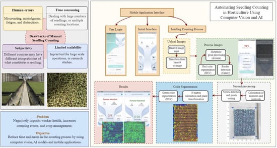
Automating Seedling Counts in Horticulture Using Computer Vision and AI

Abstract

The accelerated growth of computer vision techniques (CVT) has allowed their application in various disciplines, including horticulture, facilitating the work of producers, reducing costs, and improving quality of life. These techniques have made it possible to contribute to the automation of agro-industrial processes, avoiding excessive visual fatigue when undertaking repetitive tasks, such as monitoring and selecting seedlings grown in trays. In this study, an object detection model and a mobile application were developed that allowed seedlings to be counted from images and the calculation of the number of seedlings per tray. This system was developed under a CRISP-DM methodology to improve the capture of information, data processing, and the training of object detection models using data from six crops and four types of trays. Subsequently, an experimental test was carried out to verify the integration of both parts as a unified system, reaching an efficiency between 57% and 96% in the counting process.

1. Introduction

Food security is one of the most significant challenges for modern societies because the world population is growing exponentially [1]. In 2050, it is projected that over 10 billion individuals will live on the planet [2,3], with more than 70% residing in urban areas [4,5]. This global challenge will also be aggravated by water scarcity and changing weather conditions, posing a significant threat to food security [6]. In this sense, new research opportunities and the incorporation of new technologies that are able to improve agricultural production are key to developing sustainable intensive horticultural systems [7,8,9,10,11]. In addition to this, it is important to consider that vegetables are essential for the global population [12] and are among the most popular cultivated crops today. They are seasonally grown [13], resulting in a discontinuous and intermittent supply, leading to highly variable costs throughout the year. Because of this, it is important to employ diverse growing techniques and incorporate greenhouse growing methods or vertical farming to maintain continuous vegetable production and supply [14]. In this sense, producing seedlings in nurseries is an alternative that could enable uniform and timely transplantation in either soil or soilless (hydroponic or organic substrate) cultivation systems. However, seedling cultivation is laborious and costly [15], as vegetable seedlings must be handled individually in trays to assess optimal plant quality. To maximize profitability, producers exhaustively monitor the crop before its commercialization, carrying out visual counts that allow them to determine the effectiveness of applied management strategies and, thus, define the final sale price based on the number of plants. However, the process of counting crops is both time-consuming and visually demanding, particularly when dealing with a high volume of seedling trays [16]. In addition to this, counting is susceptible to human errors caused by factors such as visual fatigue, distractions, and subjectivity. Such errors can have adverse effects on the quality of the product and its overall profitability [17]. Therefore, there is a great need to develop a tool that can overcome these issues. In this sense, recent advancements in computer vision in agriculture have led to the emergence of innovative applications, ranging from experimental research to commercial applications, offering promising solutions to enhance various aspects of horticultural activities. In this regard, [16] this paper discusses the increasing use of artificial intelligence techniques and robotic systems in agriculture, specifically focusing on machine learning (ML) and deep learning (DL) algorithms. ML and DL have significantly improved agricultural tasks, such as plant disease detection and classification, weed–crop discrimination, fruit counting, land cover classification, and crop–plant recognition. Other tools, such as remote sensing, offer scalability and are less labor-intensive, as described in [18,19] because they use satellite or aerial imagery, drones, or specialized sensors to capture crop density and health data. Therefore, leveraging machine learning and computer vision algorithms to count crops in images or video feeds automatically is becoming more popular due to its automation capabilities. Similarly, experimental robotic vehicles have emerged as key players, demonstrating their ability to efficiently navigate through plantation lines by seamlessly integrating machine vision with GPS information [20]. In addition to this, other platforms have been designed for remote plant inspections, leveraging high-quality thermal imagery data to identify potential issues and ensure optimal plant health [21]. For instance, [22] developed and built an economic farming robot that had the capability to monitor vegetables throughout their entire growth cycle, performing precise irrigation according to the growth stage of each individual plant and enabling precision cultivation in limited spaces. Furthermore, the integration of machine learning object detection through computer vision with Unmanned Aerial Vehicle (UAV) RGB imagery has proven invaluable for rapid plant classification based on the maturity level in broccoli heads [23], sugar content prediction in grapevines with automated machine learning (AutoML) [24], automatic disease identification on wheat plants using a deep convolutional neural network (DCNN) [25] and the early prediction of wheat yield using ML methods with multi-sensor data fusion [26]. These cutting-edge technologies empower producers to make informed decisions based on data-driven insights. Therefore, there are several tools that are currently applied in this field, with the potential to generate substantial improvements in the productive process, especially in the growing stages of crops or seedlings. However, it is important to consider that the applicability of crop counting is a complex task that needs further efforts by researchers, given that crop variability, overlapping plants, and adverse weather conditions can all impact the accuracy of counts. Despite these challenges, the applications of crop counting are vast. It contributes to precise yield predictions, which are crucial for pricing, marketing, and resource allocation [27], also aiding in the efficient distribution of resources such as water, fertilizers, and pesticides. Therefore, crop counting enables farmers to manage their fields effectively and sustainably.

A way to overcome the limitations of crop counting could be the use of computer vision techniques (CVT), which enables computers to interpret and understand visual data from the world around them. One common approach corresponds to the use of image processing algorithms that extract features from images and perform various analyses [28], such as color space conversion (to identify and isolate specific colors of interest) [29], homography (to correct any perspective distortion in the input image) [30,31], local and global descriptors (to identify and classify objects) [32], and machine learning techniques [33]. Combining these models allows a system to automatically detect seedlings, adding greater precision and flexibility to the production process.

These algorithms can perform large counting processes consistently without fatigue or distraction, incorporating objectivity when determining the individuals that complete the production process. Efforts have been made in the literature to combine these techniques to apply CVT to agro-industrial processes. For example, in [34], a deep convolutional neural network was used to automate counting tomato fruits even when occlusion occurred (because of branches or foliage). Also, [35] used deep learning techniques to detect highly occluded immature tomatoes. However, this process involved high computational resources due to non-optimized object detection algorithms, making it difficult to apply in real operating environments. Other authors, such as [36], have performed leaf counting by applying Circular Hough Transform (CHT), focusing mainly on the phenotypic properties of plants to predict their interaction with the environment. Another study focusing on earlier estimations of rice yield carried out by [37] proposed an efficient method that used computer vision to accurately count rice seedlings in a digital image, which involves using UAVs equipped with RGB cameras to capture images of the rice field during the seedling stage. These images were then processed using a regression network (Basic Network) inspired by a deep, fully convolutional neural network. This network generates density maps and estimates the number of rice seedlings in each UAV image, reaching an average accuracy higher than 93%. Also, in rice, [38] were able to detect seedlings in paddy fields using transfer learning from two machine learning models (EfficientDet-D0 and Faster R-CNN), obtaining a mean average precision (mAP) of 95.5% and almost 100% in training alongside 83.2% and 88.8% when EfficientDet and Faster R-CNN models were tested, respectively. In [39], a computer vision-based peak detection algorithm was applied to locate the crop rows and plant seedlings using high-resolution UAV images in two different crop types: maize and sunflower. The proposed method obtained R-squared values of 0.76 for the maize dataset and 0.89 for the sunflower dataset. In another study, using a deep learning algorithm, [40] developed a method for detecting and counting tree seedlings in RGB images, including dragon spruce, black chokeberries, and Scots pine. The proposed method utilized data augmentation techniques and a YOLOv5 object detection network to achieve high accuracy in seedling detection, with an average accuracy of 95.1%. Although previous methods have significant advantages, there is a need for further research on object detection models applied to vegetable production at an industrial level. While some systems are already in use, they are not widely available and can be costly. Despite the significant advantages of using these methods, object detection models applied to vegetable production are still scarce. Therefore, more research is needed to develop affordable and scalable object detection models for vegetable production. For these reasons, this study aims to develop a new method that is capable of reducing the time and error associated with manual seedling counts under greenhouse conditions using object detection models and a mobile application.

2. Materials and Methods

2.1. Seedling Growing Process and Traditional Seedling Counting Method

The nurseries purchase certified seeds from an external supplier to begin the seedling process. Afterward, the local laboratory confirms the germination percentage with a simple germination test before production. The initial output step involves determining the type of trays on which the crop is established during sowing. To produce vegetable crops, trays of 486, 260, 104, and 72 cells are currently used (where the number corresponds to the total number of cells or seedlings they can contain). On trays 486 and 260, industrial tomato, watermelon, broccoli, and lettuce are preferably produced. In contrast, trays 104 and 72 are mainly used to produce tomatoes, pepper, and cabbage. Next, the tray is covered with the substrate, and it continues to the implanted machine, where respective holes are made in each tray cell, and one or several seeds are deposited in each cavity. After the trays are checked, the substrate covers the seeds again. Once this process is completed, the trays are grouped on a pallet and transferred to a germination chamber where temperature and humidity are regulated. In this chamber, the trays are kept for 1 to 3 days (depending on the variety and species). Finally, the trays are placed into the corresponding greenhouses, recording information on (i) client ID, (ii) the type of tray, (iii) the total number of trays, (iv) species, (v) variety, and (vi) planting date.

Once the nursery production stage is completed, the counting process begins, which takes place 10 to 12 days after the planting date. This information is strategic for the companies since it allows them to measure the impact of the productive management defined at the field level and set the projected sale prices to the market. To achieve the above, the farmers calculate how many trays must be counted to evaluate a complete batch. For sample selection, trays are randomly selected to obtain a sample for visual counting, excluding trays located on the edge of batches due to the border effect. For example, if a consignment of 100 trays is considered, the assigned count percentage is 10. However, traditional production systems contemplate the production of large quantities of seedlings to supply the local market, so the simultaneous evaluation of batches is a complex task for the industry. In this sense, a medium-sized company can sell up to 150 million plants per season, producing 650,000 trays. Of this total, 10% must be visually evaluated by the workers, which means that 65,000 trays must be individually assessed by specialized workers (approximately 15 million seedlings). This task requires at least ten farm workers dedicated to visual counting tasks (considering an average count capacity of 1.5 million plants/worker/season).

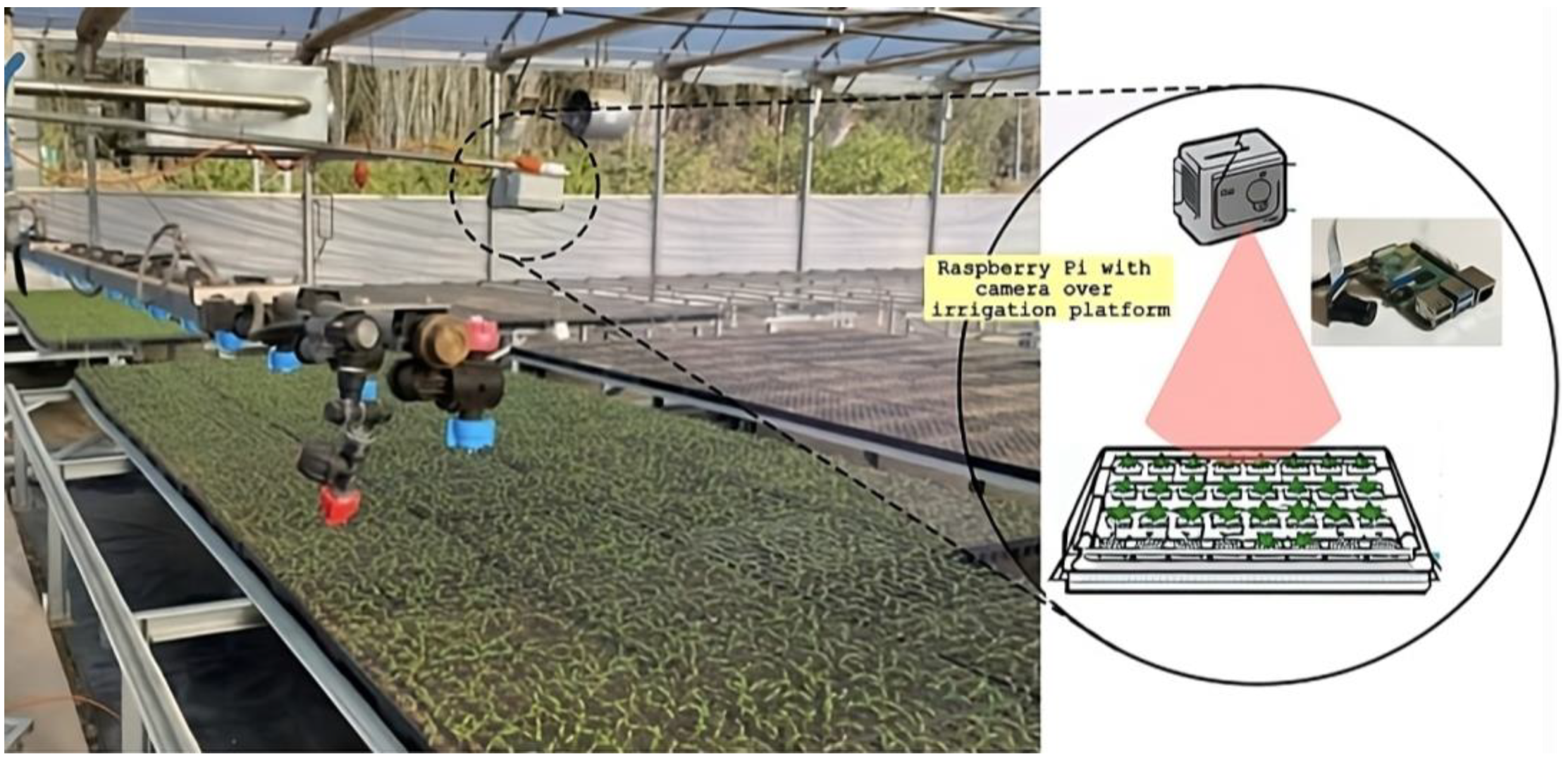
2.2. Hardware Development

The initial phase of the system’s development involves systematically gathering information. This can be accomplished by incorporating a hardware–software system that collects information automatically at the field level. Raspberry Pi 3 B+ hardware was deployed with a Raspberry Cam V2 RGB and an autonomous power supply system. This microcomputer can execute most typical computer tasks, facilitating integration with peripherals. Once these steps are completed, the integration of the Raspberry Cam V2 RGB image capture device follows. The Raspberry Pi must be accessed using the sudo raspi-config command for camera configuration. Once the command is set, a screen with the Raspberry Pi configuration is displayed, where the user can access the interface options that allow peripheral devices to be configured:

• from picamera import PiCamera
• from time import sleep
• import datetime
• now = datetime.datetime.now()
• path = “/home/pi/Desktop/imagenes/”+str(now)+”.jpg”
• camera = PiCamera()
• camera.start_preview()
• sleep(5)
• camera.capture(path)
• camera.stop_preview()

The first step was to create a folder on the Raspberry Pi. The command mkdir creates a folder on the Raspberry Pi through the command line. Once the folder is created, the libraries that allow control of the Raspberry Pi camera in Python are imported. The sleep library delays the code execution while taking the picture. Additionally, the dateTime library addresses the issue of file overwriting within the pre-existing folder, as the captured image is always saved with the same name, leading to file overwriting.

This process started with a request to find out if there was an Internet connection, and the folder was entered to read the images if there was an active connection. After the image was stored in the local folder, the association was queried again to send the image to the database server and then delete the image from the local folder. The execution of this process is essential since, if the pictures are not downloaded to a remote server, the memory of the local device could fill up, preventing the capture of new information.

It should be noted that It is necessary to periodically execute both codes to capture and send images to the server’s database. To achieve the above, Cron.

• tab was used [41] with the following code:
• x/5 * *x * * python /home/pi/Desktop/capture_images.py
• x x/4 x x * python /home/pi/Desktop/send_images_to_server.py

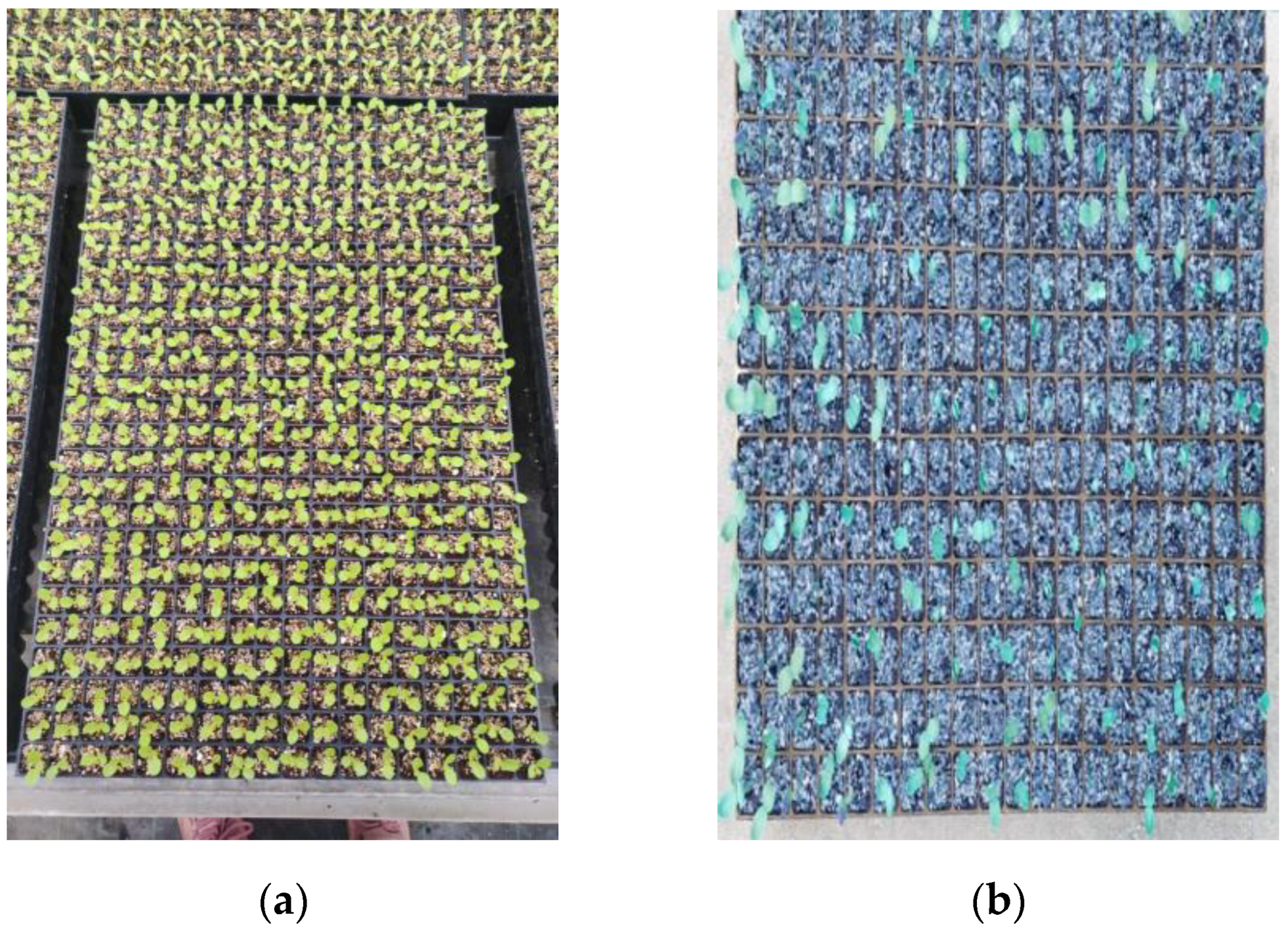
2.3. Description of the Dataset, Initial Filters, and Increasing Dataset Quality

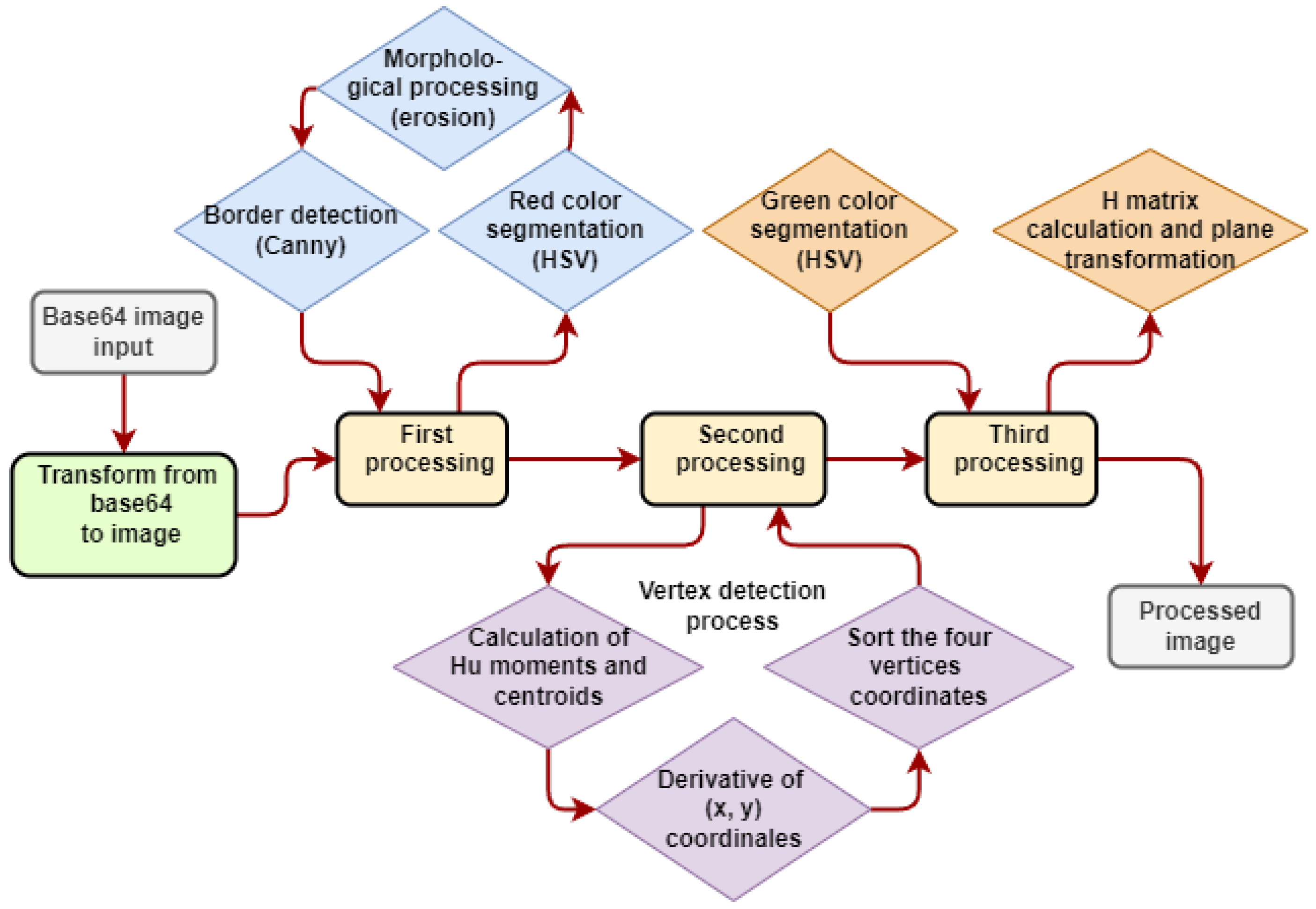
For the dataset’s construction, the device is mounted on a mobile platform (tripod) and placed in a fixed position over the production trays. The camera configuration captures information using a resolution of 8 megapixels. The process of obtaining images is automated with a temporal frequency of 5 minutes. It should be noted that the agricultural work was carried out normally, which is why the dataset was later filtered to eliminate images where obstructions, errors in the positioning of the device, duplicate data, and blurred images occurred. Information was obtained using the seedlings of tomato, broccoli, watermelon, pepper, lettuce, and cabbage grown in trays of 72, 104, 260, and 486 cells. Details corresponding to the crop–tray combination are presented in

Table 1. Tray type used for each crop.

Crop	Tray Type
Tomato	72, 104, 260, 486
Broccoli	260
Watermelon	260
Pepper	104
Lettuce	260
Cabbage	104

.

Once the dataset was obtained, algorithms and transformations were applied to improve the classification results. This process was divided into different steps, including color segmentation (HSV), homography, morphological transformation, and global descriptors. These techniques corrected the perspective, improved image quality, represented key features, and separated objects of interest from the background. The workflow proposed for image analysis is detailed in Figure 1, and each step is detailed below.

2.4. Color Space

HSV is a model used in computer vision to map colors regarding their hue, saturation, and brightness rather than RGB (red, green, blue) values [42,43,44]. The HSV color space is beneficial for computer vision since it simplifies the visual information process. Moreover, saturation and brightness in HSV can be employed to segment objects in the image based on their texture and luminance. For example, saturation can be used to differentiate between high and low saturation regions and the brightness value can be used to distinguish between higher and lower brightness areas. In this sense, to implement HSV segmentation, the edges of these images must be clearly identified. For this, markers corresponding to red circles were manually inserted in each corner of the tray. Subsequently, HSV was used to isolate the frequencies associated with the red color and segment the input vertices (first processing—stage one, Figure 1). Any color equal to red was represented as a white value (maximum possible), and any color different from red was plotted as black (minimum value). However, colors similar to red were also segmented during the process, which is why the processed image contained noise, which was removed to determine the edges correctly. HSV segmentation was also applied in the third processing—stage two (Figure 1)—to change the image color space by increasing the saturation of the green to highlight this color and facilitate the identification of pixels corresponding to the seedling.

2.5. Morphological Transformation

A morphological transformation technique was applied to analyze the shape and structure of objects in an image [45,46]. These techniques include dilation, erosion, opening, and closing [47,48]. In this sense, erosion is commonly used to denoise or separate connected objects in an image. All additional elements that did not correspond to the tray vertices were removed, leaving only 4 points on the image (First processing—stage two, Figure 1). In the vertex detection and points sorting block, the corresponding moments were calculated, from which the (x, y) coordinates of the vertex were derived. These coordinates were stored in two separate arrays. Subsequently, once the coordinates of all objects had been obtained, they were sorted in the following format: (x1, y1) for the upper-right vertex, (x2, y2) for the lower-right vertex, (x3, y3) for the upper-left vertex, and (x4, y4) for the lower-left vertex. Once the points were sorted according to this criterion, an image was generated.

2.6. Canny Technique to Detect Tray Borders

To obtain the edges of each vertex, the exact spatial coordinates of the centers must be determined. To achieve this, the Canny edge detection algorithm was applied (first processing—stage three, Figure 1) using a multi-stage sub-process [49]. The first step was to apply Gaussian smoothing to the image. This was performed to reduce noise and prepare the image for gradient calculation. Finally, thresholding was applied to the image’s high and low values, and then these thresholds were set to delimit the edges of the four vertices of the cuttings tray.

2.7. Local and Global Descriptors

Afterward, the central points of each figure identified in the previous stage were determined. For this, descriptors were used. In this sense, local descriptors are a feature extraction technique that focuses on extracting data from specific regions of an image, such as the edges, points of interest, and texture patterns. These local features provide a detailed description of the visual characteristics of an image. SIFT [50,51], SURF [52], ORB [53,54], and other techniques are commonly used as local descriptors. By contrast, global descriptors extract features from the entire image, such as the color histogram or the spatial distribution of textures. One typical example of a global descriptor corresponds to Hu moments [55,56,57]. Local and global descriptors are necessary for computer vision because they allow the extraction and representation of different types of visual features from an image, which is essential for many CVT applications. For the second processing—stage one (Figure 1)—Hu moments were used to determine the x-y coordinates of each vertex’s centroid, allowing the exact spatial coordinates of the centers to be obtained.

2.8. Perspective Transformation and Homography

Once the four vertices were obtained, the homographic transformation [58,59] was performed to fix irregularities in the image that could affect the counting process (third processing—stage one, Figure 1). Occasionally, when taking a photograph, the perspective of the tray resulted in a rhomboidal shape, which could create difficulties when counting seedlings. This is why the perspective transformation rectified this by changing the plane containing the image into a frontal plane. Using the homography transformation, the four pairs of points corresponding to the image’s vertices were used to calculate the H matrix values and perform perspective transformation.

2.9. Machine Learning Processing

Machine learning or automatic learning is a branch of artificial intelligence that focuses on developing algorithms and models that allow machines to learn and improve their performance in specific tasks through experience and data [60,61]. The open-source software library TensorFlow [62] was used to deploy models and classify pre-processed images. For this research, convolutional neural networks (CNNs) were used. CNNs are a type of neural network that is particularly well-suited to image recognition and classification tasks [63,64]. When working with RGB images in TensorFlow, convolutional neural networks (CNNs) typically take input data as 3D tensors with dimensions (height, width, channels), where the channels correspond to the following three colors: red, green, and blue. The input tensor is passed through several layers of convolutional and pooling operations, which allow the model to learn features from the images, followed by one or more fully connected layers for classification or regression tasks. The TensorFlow library provides a comprehensive set of tools and functions to build and train CNNs with RGB images, making it a popular choice for image recognition and computer vision tasks. This study used a labeled image dataset to update the CNN model weights through backpropagation and stochastic gradient descent. The selection of a suitable classification model involved the use of pre-trained TensorFlow models capable of handling 640 × 640 images, such as ResNet, SSD MobileNet, and EfficientNet. Due to this limitation, the 8-megapixel image resolution could be reduced when using the model. Moreover, several factors must be considered, as highlighted in the following items.

(a) Choosing Tensorflow models: TensorFlow has several pre-trained models for classification tasks. The architecture of each model varies, with differences in the number of layers within the convolutional model. A model with more layers tends to produce a higher accuracy but at the cost of slower processing times. Conversely, models with fewer layers run faster but can compromise the algorithm’s accuracy.

(b) Training and validation TFRecord files: TFRecord files are a binary format used by TensorFlow to detect labeled survey objects in the Roboflow platform (https://roboflow.com/). This tool enables image tagging for object detection models by specifying the classification requirements. Once labeling is complete, the images are downloaded with a CSV file containing the filename, width, height, class, xmin, ymin, xmax, and ymax. These coordinates indicate the position of labeled objects in the respective images. The TensorFlow documentation provides a code for the conversion process to convert the training and validation images’ corresponding CSV files into TFRecord files.

(c) LabelMap file: LabelMap is a file that allows the classes the object detection model identifies to be written. It is important to note that LabelMap files work slightly differently from one library to another. The structure used for the detection of the seedlings is shown below:

• Item: {
• name: ‘crop
• id: 1
• }

Since only a single object needs to be detected, the file only contains one item. However, if the user wants to add more objects to the detection, other items must be incorporated into the file by adding the name of the study object with a different ID.

(d) Configuration file pipeline.config: The pipeline.config file contains the entire architecture of the convolutional neural network. Each detection model has a pipeline.config file that must be configured before training the model and is available when downloading the model from Google Colab. Within the file, there are several different hyperparameters (HP) that can be optimized to favor detection. HP values correspond to the following attributes: (i) the number of classes, (ii) batch size, (iii) checkpoint, (iv) LabelMap, (v) training TFRecord, and (vi) validation TFRecord. In this research, these hyperparameters were not optimized to compare each model with its initial configuration.

Finally, the object detection model was trained once the file was configured according to the data science methodology. Once this training was finished, it was necessary to save the model to perform the inferences on new images loaded in the model inference code.

2.10. Data Science Methodology Applied

The CRISP-DM (Cross-Industry Standard Process for Data Mining) is a widely used methodology for implementing data mining projects [65]. Implementing the CRISP-DM methodology involves several steps, including business understanding, data understanding, data preparation, modeling, evaluation, and deployment. First, the business of the understanding stage defines the problem and the project objectives. Next, the data understanding stage involves gathering and exploring data to understand their quality and characteristics better. This stage includes data collection, description, exploration, and quality assessment. The goal of this stage is to identify any issues within the data and determine whether the data are suitable for the project. The data preparation stage involves cleaning, transforming, and integrating data for the modeling stage. This stage aims to create a high-quality dataset that can be used to develop a model. The modeling stage involves building and testing a predictive model based on the prepared dataset. This stage includes model selection, model training, and model testing. The evaluation stage comprises assessing the model’s performance and determining whether it meets the project objectives, identifying any issues, and deciding if it can be deployed in the production environment. Finally, the deployment stage involves implementing the model in the production environment.

2.11. Model Evaluation

According to the CRISP-DM methodology, one of the most used evaluation metrics in computer vision and machine learning when evaluating the performance of object detection models is mean average precision (mAP). This value can be used to measure how well the model identifies objects of interest in an image and is useful when there are multiple objects of interest present. The mAP score is computed by first calculating the average precision (AP) for each object class in the dataset. The average precision for a given class measures how well the model can detect objects of that class at various levels of precision and recall. The model’s output was sorted by confidence score to calculate AP, and then a precision–recall curve was generated by varying the detection threshold. The AP was then calculated as the area under this curve. Once the AP was computed for each object class (in this case, only one class corresponded to the seedling), the mAP score was calculated as the average of the AP scores across all classes. This measured the model’s overall performance across all object classes. In practice, mAP is often used as a primary metric to evaluate object detection models as it provides a simple and effective way to compare the performance of different models on a given dataset.

2.12. Tools and Frameworks

Afterward, the next step is to execute the model, which counts the seedling images continuously and accurately. This research used the Google Cloud Platform, specifically utilizing two primary services: Cloud Storage and AI Platform. Within the Google Cloud Platform, the Cloud Storage service allows the trained model to be saved with the “LabelMap” file. Once the files are stored, the AI platform can be used to run artificial intelligence model inference. For this, a TensorFlow “notebook” was created to write all the inference codes (which are available at https://github.com/ffuentesp7/Counting-seedlings). In addition, to develop the mobile application, the Flutter framework was used for the user views or Frontend, and Node js was used to build the logic or Backend. The Backend is an API REST with several endpoints that aid in obtaining specific information needed by the Frontend, collecting this information from the database manager. Inside the API, all the project logic that allows responses to be made to the client according to the data entered is contained.

3. Results

3.1. Hardware Mounting and Field Deployment

With new CVT methods, RGB images have gained value in developing new cost-effective strategies or technologies for crop management and monitoring [66]. In this sense, RGB images are particularly valuable in agricultural environments since they easily differentiate vegetation from other surrounding objects [67,68,69,70]. Considering the above, a replicable, scalable, and interoperable device was used for this research to capture RGB data. However, it must be considered that these devices are not adapted to the operational ranges commonly found in commercial greenhouses. Due to this fact, the proposed device was specially adapted, including a case to optimize information collection. During the development of the experiments, it was observed that relative humidity varied between 31% and 99% and temperature between 10 °C and 41 °C. Humidity control was particularly problematic due to moisture condensation inside the case. In this study, humidity was successfully controlled by installing silica bags inside the device. Afterward, to guarantee the device’s operation, an autonomous power supply system was installed in the device. Additionally, the device was connected to the local power grid to avoid data loss.

For the near real-time transmission of information, a local Wi-Fi network was used. To achieve this, a conventional antenna was installed to provide connectivity inside the greenhouse. The signal’s intensity and the connection’s stability were also evaluated, demonstrating that factors such as machinery operation and other IoT devices’ connection to the network did not allow a stable connection to regularly send information to the server. For this reason, a Wi-Fi repeater had to be installed in each greenhouse. Finally, a mobile metallic tripod was designed to facilitate agricultural operators’ use of the device. This structure allowed easy positioning and movement for each evaluation. It should be noted that the total cost of the device was 75 USD, which considers the microcomputer, camera, cables, wheels, and metal structure.

3.2. Initial Dataset

The device captured a total of 10,000 images. However, since this dataset consisted of images systematically captured every 5 minutes, initial filters were applied before pre-processing to ensure the quality of information. The first filter removed 3000 images captured between 7 p.m. and 7 a.m. when there was insufficient light to differentiate objects in these images. Subsequently, duplicate pictures were eliminated, ensuring that the model avoided overfitting and that the evaluation metrics were both reliable and robust. Considering this, 2880 images were eliminated due to their similarity caused by the temporal frequency of 5 minutes, which was established because of the rapid growth of the crop in its early stages of development. Another 3420 images were removed due to noise, such as workers, agricultural tasks, machinery movement, and strange objects within the images. Finally, 700 images were selected for pre-processing after applying the filters. Of this total, 80% of the total dataset was destined for the training set, which served as the foundation for the machine learning model to learn underlying patterns. An additional 15% was reserved for the validation set, used for hyperparameter tuning and providing an unbiased evaluation of the model during its training phase. The remaining 5% was designated as the test set to assess the model’s final performance.

3.3. Data Pre-Processing

One of the main drawbacks when applying different algorithms and object detection models is the image’s processing complexity. Often, there are multiple trays in the pictures, and there is no clear pattern to segment the central tray, as seen in Figure 2.

As described before (in Figure 1), a workflow was applied to improve the image quality and address these issues. In the first place, four red vertices needed to be manually inserted into each image to delimit the tray. This process was successfully carried out for all 700 images. Afterward, images were subjected to the HSV, erosion, and border detection (Canny) transformations to isolate these objects and determine the images’ centroids. To achieve the above, a second process had to be carried out where Hu moments were used to determine the exact coordinates corresponding to the vertices of the trays (Figure 3).

Another factor to consider is the image perspective. As seen in Figure 4a, the plane containing the tray was much broader at the bottom and decreased at the top of the image. Using the homography transformation, the four pairs of points corresponding to the image’s vertices were used to calculate the values of the H matrix and change the image to a frontal perspective. After this change was applied, each pixel of plane A (Figure 4a) was depicted in plane B (Figure 4b). This allowed everything outside the tray’s contour to be eliminated, generating a frontal image that helped visualize, in a better way, all its contents. Finally, to differentiate the green of the leaves from other colors, the image’s color space was changed, increasing the saturation of the green color to the maximum so that it could stand out from others in the image.

To create the necessary files to train an object detection model, individual seedlings were labeled in each of the original 700 images from the dataset (Figure 5). The 486-cell trays had a high occlusion of seedlings and were removed from the dataset to increase quality and reduce noise. Therefore, 550 images were labeled and categorized into 260, 104, and 72 cell formats. Finally, the number of labels for these formats reached approximately 80,000 individual labels.

3.4. Detection Model Evaluation

EfficientNet, SSD MobileNet, and ResNet are well-known computer vision algorithms that are widely used for image classification and object detection tasks [71]. EfficientNet is an object detection algorithm with higher accuracy and fewer parameters and computational resources than other methods [72]. In contrast, SSD MobileNet is a lightweight neural network architecture that is designed to run efficiently on mobile devices with limited computational resources. Finally, ResNet is a deep neural network with variable parameters requiring significant computational resources [73]. EfficientNet generally outperforms SSD MobileNet and ResNet in object detection tasks regarding accuracy. SSD MobileNet, however, is often used for image classification and localization tasks where there is a need to balance accuracy and processing speed. In this sense, to evaluate the pre-processed data used for RGB images, a dataset of 180 images featuring tomato crops in trays, each with 260 cells, was selected to test the performance of these three models. The SSD MobileNet achieved an accuracy of about 91% for the images in the trays. However, the SSD MobileNet’s effectiveness was slightly reduced for other crops, such as peppers, with an accuracy ranging between 78 and 81%. Figure 6 shows the classification and localization loss metrics observed during the execution of the SSD MobileNet convolutional model with training and validation sets tested for over 24,000 epochs.

Therefore, the model performance was tested by training all the images in the dataset and showing the results of loss classification, loss localization, and mean average precision (mAP).

Table 2. Benchmark of object detection models.

Metrics	EfficientNet	SSD MobileNet	ResNet
Loss Classification	0.10	0.08	0.13
Loss Localization	0.13	0.05	0.07
Mean Average Precision (mAP)	0.617	0.567	0.554

displays the metric values generated using the three object detection models.

The SSD MobileNet showed a balanced performance, accuracy, and processing time according to Figure 6 and the official documentation (https://github.com/tensorflow/models/blob/master/research/object_detection/g3doc/tf2_detection_zoo.md). It should be noted that there are more sophisticated models in the repository, but their implementation requires considerable computing power to perform the training. To make the model’s crop detections visible, bounding boxes were generated around each crop, as shown in Figure 7. Once the object detection model was selected, it was deployed in a production environment to count the seedling images.

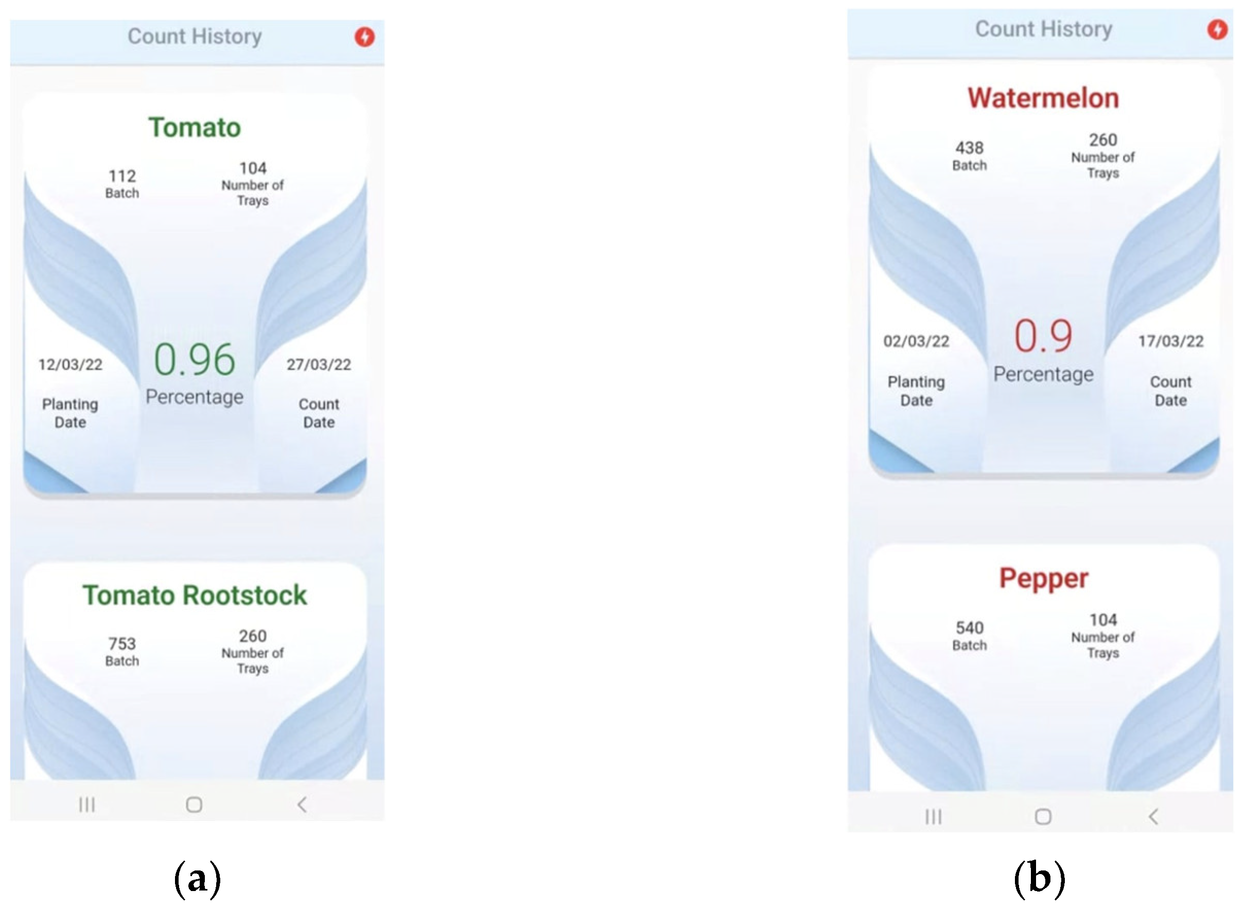
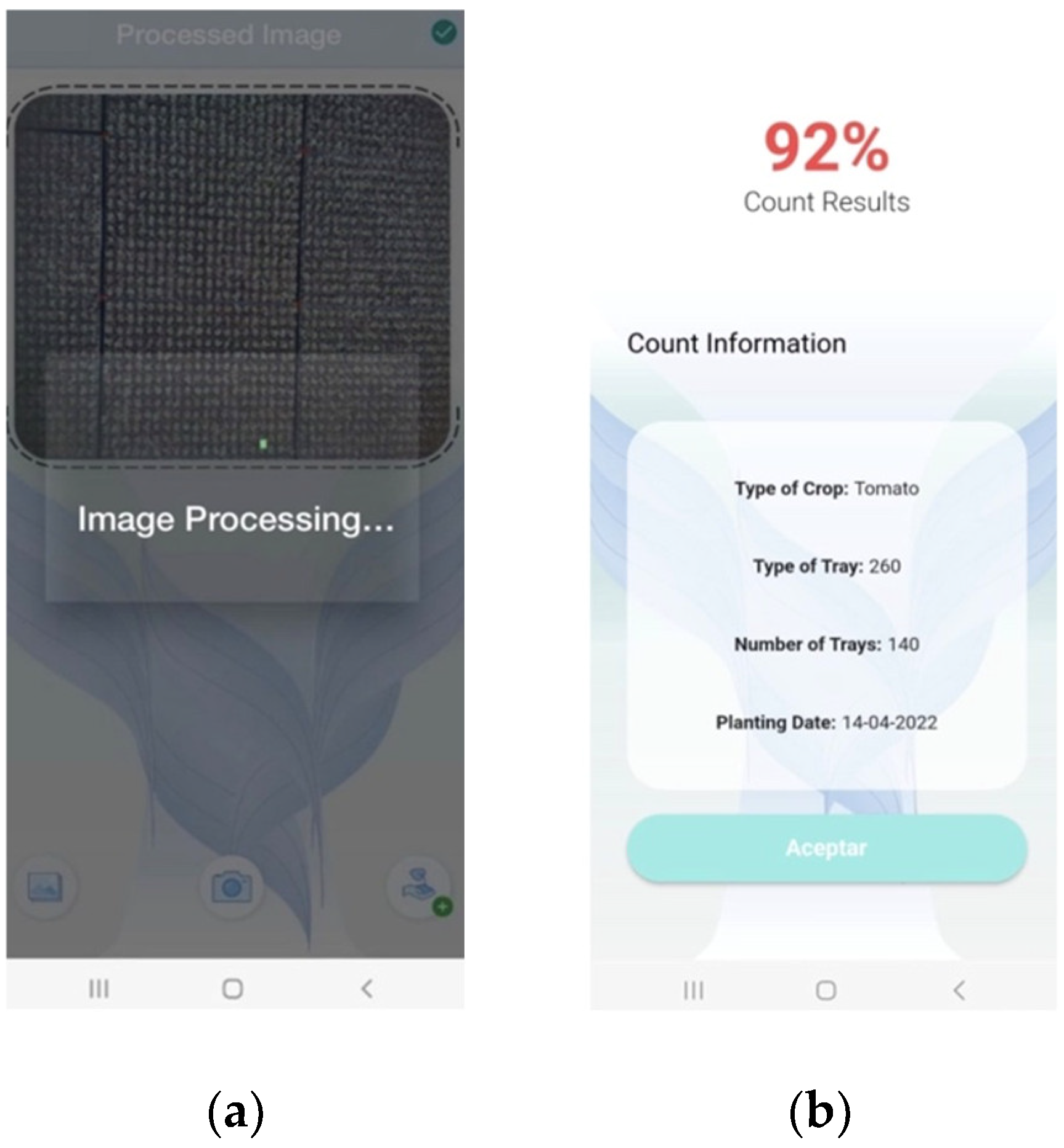
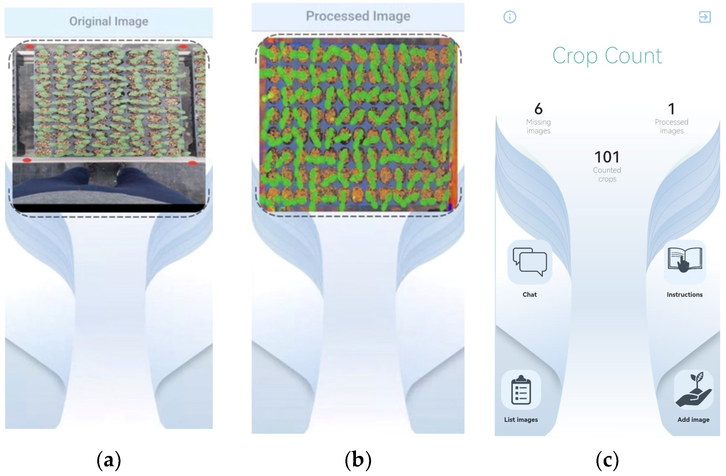
3.5. Development of A Mobile Application

The application development process used the P × P methodology [74], as mentioned earlier. This application meets the requirements and is compatible with Android and iOS platforms. The primary functions of this application are (a) user registration and login, (b) crop counting, and (c) chatting with other company members and obtaining assistance. Figure 8 shows some of the main views of this application.

The application login is on the left, and the most important functionalities are shown in the center and to the right. The application was designed to be as simple and clean as possible to favor user experience and not make capturing images and obtaining results more complex. The primary objective was to deploy the proposed plant detection model through a faster and more user-friendly interface. The app’s workflow involves user registration and the beginning of a new count. After filling out the form, the user must upload the images captured by the mobile device. The server-side processing counts the seedlings in each image and sends the total number to the user. The application sums up the count as the user loads the images, and at the end of the count, the app displays the percentage, allowing the user to estimate the average number of seedlings per tray. Figure 9 shows the different results of the proposed application when counting multiple crops. As seen in the case of tomatoes, the results had a precision of over 90%.

3.6. Deployment and Final Field Testing

This section evaluates the developed product when integrated with the proposed model described to corroborate the general objective’s achievement level. For the experimental test, a case was tested to count a batch from a small business client. Figure 10 shows the batch information required to start the operational test, calculating the number of trays to be counted since this was necessary for manual counting and the use of this application.

The results obtained by the worker for the test shown in Figure 11 were as follows:

Table 3. Comparison between the worker and this proposal.

Test	Average Time	Number of Trays Counted	Number of Seedlings per Tray	Percentage Obtained
Industrial worker	12 min 40 s	30 trays	89	85.5%
Our proposal	9 min 35 s	30 trays	89	91.3%

shows an experiment that is designed to assess the performance of the counting application in contrast to manual counting conducted by an employee of the company. To carry out this comparison, 30 trays were randomly selected in the initial phase, which served as the study sample for the experiment. The company employee manually counted the seedlings in each tray and recorded these counts in a notebook. In addition to conducting the counting, the employee also had to consider the time to summarize the obtained information. On the other hand, the application analyzed the same set of trays, taking photographs of them and loading them into the application. The results in Table 3 show that the proposal outperformed the manual counting performed by the company employees in terms of accuracy and efficiency. Our application achieved an accuracy percentage of 91.3%, compared to the 85.5% obtained through manual counting. Additionally, the application reduced the time required to count the seedlings.

4. Discussion

Greenhouses are closed environments where plants are grown under controlled or semi-controlled conditions [75]. They provide a suitable environment for the growth of plants, but they also pose unique challenges when capturing images for CVT [76]. The main challenges observed in this study regarding the implementation of CTV over a greenhouse were:

1. Lighting conditions [77,78]. Greenhouses typically have complex lighting conditions due to the presence of natural and artificial light sources. Natural light can cause shadows, reflections, and variations in color and intensity [79,80]. Artificial light creates glare and interferes with image quality [81]. The light spectrum used in greenhouses also differs from the natural light spectrum [82,83], which can cause difficulties when capturing images accurately. Other research has also faced lighting problems when using various computer vision techniques; for example, [84] implemented a method based on image analysis to identify weeds in cabbage and carrots under open-field experiments. This was performed using a device that provided controlled lighting (avoiding natural issues), which could classify objects with a precision between 51% and 95%. In [85], computer vision techniques were used to develop an automatic phenotyping system combining the automatic procedure with a high-performance segmentation algorithm in greenhouse tomatoes. In this case, the developers reported that during day-time measurements, data collection faced different illumination conditions because of the influence of external light (clouds, daily and seasonal variations in the intensity of the sunlight), indicating significant impacts on data quality acquisition. Therefore, for this study, the selection of images was indeed subject to light conditions, and the images of the initial dataset that were subject to insufficient light had to be discarded (2880 images).

2. The need for high-quality and labeled training data. Collecting and annotating such data can be time-consuming and require expert knowledge, as plant species can be highly diverse and require careful identification and classification. As demonstrated in this paper, it is necessary to use a dataset that is representative of the plant species in order to be classified and correctly labeled. However, our research took a different approach by evaluating several crops in a greenhouse, unlike previous studies that have assessed only one species or type of fruit.

3. The design of the devices used over the crop to be monitored was also an issue identified in this study. For this case, the images had to be taken in a lateral position due to the crop conduction system, for which light had to be supplemented with a led bar to maintain homogeneous data-capturing conditions. In addition to this, consideration had to be given to the image perspective, given that an image taken from an inclined perspective could generate errors in the counting process; in this sense, the application of pre-processing the image dataset was successful and allowed the precise implementation of the counting algorithm.

4. Environmental factors in greenhouses. High humidity levels can fog up camera lenses and reduce image clarity. Additionally, dust, dirt, and other particles can obscure the image and cause a loss of image quality.

5. The crop’s growth conditions. This research faced a significant challenge, particularly when growth was advanced, compared to other studies with lower occlusion [86].

Addressing these challenges allowed us to optimize the seedling counting process, for which the use of computer vision models (CVT) was fundamental. In this sense, using CVT to detect objects in images has found broad applications in recent years. In the case of greenhouses, CVT has the potential to reduce labor costs and worker fatigue. This is because monitoring plant growth and health in greenhouses requires significant manual labor. However, automating this process can reduce the number of workers needed to monitor plants. According to the literature, computer vision techniques combined with machine learning models have been used to solve complex problems regarding the classification and identification of crops in greenhouses. In addition to this, object detection models also play an important role in image detection, where models such as EfficientNet, SSD MobileNet, and ResNet have different performances that can be compared regarding two crucial computer vision tasks: classification and localization. For this study, tomato detection using SSD MobileNet performed better than those presented in the study by [87], where segmentation of the CVT space was also conducted. Nonetheless, the need for a sufficiently complete machine learning model and the limited quality of the dataset in terms of balanced images negatively impacted these segmentation results. Regarding the mean average precision, which is used to test the performance on object detection tasks, which in this case was labeling objects, EfficientNet generally outperforms SSD MobileNet and ResNet due to its compound scaling approach and advanced regularization techniques such as stochastic depth and mixup. In localization and classification tasks, the aim is to minimize this loss, which measures the model’s performance. Therefore, SSD MobileNet is best suited to this task.

In terms of the performance of the model, the comparison made to assess the precision when counting between the proposed method and a greenhouse worker indicated that a higher precision in counting was achieved by the proposal developed in this work, with over 90% precision when counting seedlings, saving time by over three minutes. Lastly, as demonstrated in this paper, it is necessary to use a dataset that is representative of the plant species to be classified and correctly labeled. However, our research took a different approach by evaluating several crops in a greenhouse, unlike previous studies, which have assessed only one species or type of fruit. Finally, these experiments can be replicated through our repository and reproduced as open-source code.

5. Conclusions

In this work, a deep-learning mobile application with SSD MobileNet was applied to detect crops in seedling trays. Our proposal demonstrates that while there have been notable advancements in different components of automatic plant detection, implementing such a system within a greenhouse has significant challenges. Addressing them requires more than simply improving individual components and demands particular attention to the experimental arrangement and automatic classification technology. When testing our model with the generality of greenhouse crops, the detection accuracy results ranged from 57 to 96% according to the type of crop and the tray in which it was located. Thus, the size and variability of the dataset and the surface where the plant was located were the elements that had the most decisive impact on our classification results. Hence, the objectives set in this study were accomplished. Nevertheless, several paths for further research could enhance the existing system’s performance. For instance, future research could focus on detecting pests and diseases early or establishing a control mechanism before significant losses occur in crop yields, in addition to examining the machine learning model and its integration with computer vision subsystems. This application focused on object detection and counting rather than recent classification research. However, it is worth noting that the functionality and user interface of the mobile application could be extended or enhanced in the future to include additional features, such as the classification of seedlings based on certain criteria if deemed necessary for specific agricultural applications.

References

1. Khan, M.M.; Akram, M.T.; Janke, R.; Qadri, R.W.K.; Al-Sadi, A.M.; Farooque, A.A. Urban Horticulture for Food Secure Cities through and beyond COVID-19. Sustainability 2020, 12, 9592. [Google Scholar] [CrossRef]
2. Boretti, A.; Rosa, L. Reassessing the Projections of the World Water Development Report. NPJ Clean Water 2019, 2, 15. [Google Scholar] [CrossRef]
3. Woolston, C. Healthy People, Healthy Planet: The Search for a Sustainable Global Diet. Nature 2020, 588, S54. [Google Scholar] [CrossRef] [PubMed]
4. Huang, K.; Li, X.; Liu, X.; Seto, K.C. Projecting Global Urban Land Expansion and Heat Island Intensification through 2050. Environ. Res. Lett. 2019, 14, 114037. [Google Scholar] [CrossRef]
5. Dixon, T.J.; Tewdwr-Jones, M. Urban Futures: Planning for City Foresight and City Visions. In Urban Futures; Policy Press: Bristol, UK, 2021; pp. 1–16. [Google Scholar]
6. Perkins-Kirkpatrick, S.E.; Stone, D.A.; Mitchell, D.M.; Rosier, S.; King, A.D.; Lo, Y.T.E.; Pastor-Paz, J.; Frame, D.; Wehner, M. On the Attribution of the Impacts of Extreme Weather Events to Anthropogenic Climate Change. Environ. Res. Lett. 2022, 17, 024009. [Google Scholar] [CrossRef]
7. Beacham, A.M.; Vickers, L.H.; Monaghan, J.M. Vertical Farming: A Summary of Approaches to Growing Skywards. J. Hortic. Sci. Biotechnol. 2019, 94, 277–283. [Google Scholar] [CrossRef]
8. Gómez, C.; Currey, C.J.; Dickson, R.W.; Kim, H.-J.; Hernández, R.; Sabeh, N.C.; Raudales, R.E.; Brumfield, R.G.; Laury-Shaw, A.; Wilke, A.K.; et al. Controlled Environment Food Production for Urban Agriculture. HortScience 2019, 54, 1448–1458. [Google Scholar] [CrossRef]
9. O’Sullivan, C.A.; Bonnett, G.D.; McIntyre, C.L.; Hochman, Z.; Wasson, A.P. Strategies to Improve the Productivity, Product Diversity and Profitability of Urban Agriculture. Agric. Syst. 2019, 174, 133–144. [Google Scholar] [CrossRef]
10. Durmus, D. Real-Time Sensing and Control of Integrative Horticultural Lighting Systems. J. Multidiscip. Sci. J. 2020, 3, 266–274. [Google Scholar] [CrossRef]
11. Halgamuge, M.N.; Bojovschi, A.; Fisher, P.M.J.; Le, T.C.; Adeloju, S.; Murphy, S. Internet of Things and Autonomous Control for Vertical Cultivation Walls towards Smart Food Growing: A Review. Urban For. Urban Green. 2021, 61, 127094. [Google Scholar] [CrossRef]
12. Cusworth, S.J.; Davies, W.J.; McAinsh, M.R.; Stevens, C.J. Sustainable Production of Healthy, Affordable Food in the UK: The Pros and Cons of Plasticulture. Food Energy Secur. 2022, 11, e404. [Google Scholar] [CrossRef]
13. Wunderlich, S.M.; Feldman, C.; Kane, S.; Hazhin, T. Nutritional Quality of Organic, Conventional, and Seasonally Grown Broccoli Using Vitamin C as a Marker. Int. J. Food Sci. Nutr. 2008, 59, 34–45. [Google Scholar] [CrossRef]
14. Carrasco, G.; Fuentes-Penailillo, F.; Perez, R.; Rebolledo, P.; Manriquez, P. An Approach to a Vertical Farming Low-Cost to Reach Sustainable Vegetable Crops. In Proceedings of the 2022 IEEE International Conference on Automation/XXV Congress of the Chilean Association of Automatic Control (ICA-ACCA), Curico, Chile, 24–28 October 2022; IEEE: Piscataway, NJ, USA; pp. 1–6. [Google Scholar]
15. Haase, D.L.; Bouzza, K.; Emerton, L.; Friday, J.B.; Lieberg, B.; Aldrete, A.; Davis, A.S. The High Cost of the Low-Cost Polybag System: A Review of Nursery Seedling Production Systems. Land 2021, 10, 826. [Google Scholar] [CrossRef]
16. Saleem, M.H.; Potgieter, J.; Arif, K.M. Automation in Agriculture by Machine and Deep Learning Techniques: A Review of Recent Developments. Precis. Agric. 2021, 22, 2053–2091. [Google Scholar] [CrossRef]
17. Zhou, C.; Ye, H.; Hu, J.; Shi, X.; Hua, S.; Yue, J.; Xu, Z.; Yang, G. Automated Counting of Rice Panicle by Applying Deep Learning Model to Images from Unmanned Aerial Vehicle Platform. Sensors 2019, 19, 3106. [Google Scholar] [CrossRef]
18. Li, W.; Fu, H.; Yu, L.; Cracknell, A. Deep Learning Based Oil Palm Tree Detection and Counting for High-Resolution Remote Sensing Images. Remote Sens. 2017, 9, 22. [Google Scholar] [CrossRef]
19. Mekhalfi, M.L.; Nicolò, C.; Bazi, Y.; Al Rahhal, M.M.; Alsharif, N.A.; Maghayreh, E. Al Contrasting YOLOv5, Transformer, and EfficientDet Detectors for Crop Circle Detection in Desert. IEEE Geosci. Remote Sens. Lett. 2022, 19, 3003205. [Google Scholar] [CrossRef]
20. Loukatos, D.; Kondoyanni, M.; Kyrtopoulos, I.-V.; Arvanitis, K.G. Enhanced Robots as Tools for Assisting Agricultural Engineering Students’ Development. Electronics 2022, 11, 755. [Google Scholar] [CrossRef]
21. Loukatos, D.; Templalexis, C.; Lentzou, D.; Xanthopoulos, G.; Arvanitis, K.G. Enhancing a Flexible Robotic Spraying Platform for Distant Plant Inspection via High-Quality Thermal Imagery Data. Comput. Electron. Agric. 2021, 190, 106462. [Google Scholar] [CrossRef]
22. Moraitis, M.; Vaiopoulos, K.; Balafoutis, A.T. Design and Implementation of an Urban Farming Robot. Micromachines 2022, 13, 250. [Google Scholar] [CrossRef]
23. Psiroukis, V.; Espejo-Garcia, B.; Chitos, A.; Dedousis, A.; Karantzalos, K.; Fountas, S. Assessment of Different Object Detectors for the Maturity Level Classification of Broccoli Crops Using UAV Imagery. Remote Sens. 2022, 14, 731. [Google Scholar] [CrossRef]
24. Kasimati, A.; Espejo-García, B.; Darra, N.; Fountas, S. Predicting Grape Sugar Content under Quality Attributes Using Normalized Difference Vegetation Index Data and Automated Machine Learning. Sensors 2022, 22, 3249. [Google Scholar] [CrossRef] [PubMed]
25. Singh, A.; Arora, M. CNN Based Detection of Healthy and Unhealthy Wheat Crop. In Proceedings of the 2020 International Conference on Smart Electronics and Communication (ICOSEC), Trichy, India, 10–12 September 2020; pp. 121–125. [Google Scholar]
26. Fei, S.; Hassan, M.A.; Xiao, Y.; Su, X.; Chen, Z.; Cheng, Q.; Duan, F.; Chen, R.; Ma, Y. UAV-Based Multi-Sensor Data Fusion and Machine Learning Algorithm for Yield Prediction in Wheat. Precis. Agric. 2023, 24, 187–212. [Google Scholar] [CrossRef]
27. Darwin, B.; Dharmaraj, P.; Prince, S.; Popescu, D.E.; Hemanth, D.J. Recognition of Bloom/Yield in Crop Images Using Deep Learning Models for Smart Agriculture: A Review. Agronomy 2021, 11, 646. [Google Scholar] [CrossRef]
28. Wiley, V.; Lucas, T. Computer Vision and Image Processing: A Paper Review. Int. J. Artif. Intell. Res. 2018, 2, 22. [Google Scholar] [CrossRef]
29. Bhargava, A.; Bansal, A. Fruits and Vegetables Quality Evaluation Using Computer Vision: A Review. J. King Saud Univ. Comput. Inf. Sci. 2021, 33, 243–257. [Google Scholar] [CrossRef]
30. Dubrofsky, E. Homography Estimation. Master’s Thesis, The University of British Columbia, Vancouver, BC, Canada, 2009. [Google Scholar]
31. Finlayson, G.; Gong, H.; Fisher, R.B. Color Homography: Theory and Applications. IEEE Trans. Pattern Anal. Mach. Intell. 2019, 41, 20–33. [Google Scholar] [CrossRef]
32. Li, J.; Allinson, N.M. A Comprehensive Review of Current Local Features for Computer Vision. Neurocomputing 2008, 71, 1771–1787. [Google Scholar] [CrossRef]
33. Khan, A.; Laghari, A.; Awan, S. Machine Learning in Computer Vision: A Review. ICST Trans. Scalable Inf. Syst. 2018, 8, 169418. [Google Scholar] [CrossRef]
34. Rahnemoonfar, M.; Sheppard, C. Deep Count: Fruit Counting Based on Deep Simulated Learning. Sensors 2017, 17, 905. [Google Scholar] [CrossRef]
35. Mu, Y.; Chen, T.-S.; Ninomiya, S.; Guo, W. Intact Detection of Highly Occluded Immature Tomatoes on Plants Using Deep Learning Techniques. Sensors 2020, 20, 2984. [Google Scholar] [CrossRef]
36. Praveen Kumar, J.; Domnic, S. Image Based Leaf Segmentation and Counting in Rosette Plants. Inf. Process. Agric. 2019, 6, 233–246. [Google Scholar] [CrossRef]
37. Wu, J.; Yang, G.; Yang, X.; Xu, B.; Han, L.; Zhu, Y. Automatic Counting of in Situ Rice Seedlings from UAV Images Based on a Deep Fully Convolutional Neural Network. Remote Sens. 2019, 11, 691. [Google Scholar] [CrossRef]
38. Tseng, H.-H.; Yang, M.-D.; Saminathan, R.; Hsu, Y.-C.; Yang, C.-Y.; Wu, D.-H. Rice Seedling Detection in UAV Images Using Transfer Learning and Machine Learning. Remote Sens. 2022, 14, 2837. [Google Scholar] [CrossRef]
39. Bai, Y.; Nie, C.; Wang, H.; Cheng, M.; Liu, S.; Yu, X.; Shao, M.; Wang, Z.; Wang, S.; Tuohuti, N.; et al. A Fast and Robust Method for Plant Count in Sunflower and Maize at Different Seedling Stages Using High-Resolution UAV RGB Imagery. Precis. Agric. 2022, 23, 1720–1742. [Google Scholar] [CrossRef]
40. Moharram, D.; Yuan, X.; Li, D. Tree Seedlings Detection and Counting Using a Deep Learning Algorithm. Appl. Sci. 2023, 13, 895. [Google Scholar] [CrossRef]
41. Cron. Expert Shell Scripting; Apress: Berkeley, CA, USA, 2009; pp. 81–85. [Google Scholar]
42. Auliasari, R.N.; Novamizanti, L.; Ibrahim, N. Identifikasi Kematangan Daun Teh Berbasis Fitur Warna Hue Saturation Intensity (HSI) Dan Hue Saturation Value (HSV). JUITA J. Inform. 2020, 8, 217. [Google Scholar] [CrossRef]
43. Lesiangi, F.S.; Mauko, A.Y.; Djahi, B.S. Feature Extraction Hue, Saturation, Value (HSV) and Gray Level Cooccurrence Matrix (GLCM) for Identification of Woven Fabric Motifs in South Central Timor Regency. J. Phys. Conf. Ser. 2021, 2017, 012010. [Google Scholar] [CrossRef]
44. Wu, Y.; Wang, J.; Wang, Y.; Zhao, Y.; Zhang, S. Field Crop Extraction Based on Machine Vision. In Proceedings of the 2021 IEEE International Conference on Mechatronics and Automation (ICMA), Takamatsu, Japan, 8–11 August 2021; IEEE: Piscataway, NJ, USA; pp. 1–5. [Google Scholar]
45. Wilson, J.N.; Ritter, G.X. Handbook of Computer Vision Algorithms in Image Algebra; CRC Press: Boca Raton, FL, USA, 2000; ISBN 9780429115059. [Google Scholar]
46. Vizilter, Y.v.; Pyt’Ev, Y.P.; Chulichkov, A.I.; Mestetskiy, L.M. Morphological Image Analysis for Computer Vision Applications. Intell. Syst. Ref. Libr. 2015, 73, 9–58. [Google Scholar] [CrossRef]
47. Soille, P. Erosion and Dilation. In Morphological Image Analysis; Springer: Berlin/Heidelberg, Germany, 2004; pp. 63–103. [Google Scholar]
48. Chen, S.; Haralick, R.M. Recursive Erosion, Dilation, Opening, and Closing Transforms. IEEE Trans. Image Process. 1995, 4, 335–345. [Google Scholar] [CrossRef]
49. Mokrzycki, W.; Samko, M. Canny Edge Detection Algorithm Modification. Lecture Notes in Computer Science (including subseries Lecture Notes in Artificial Intelligence and Lecture Notes in Bioinformatics). Int. Conf. Comput. Vis. Graph. 2012, 7594, 533–540. [Google Scholar] [CrossRef]
50. Patrício, D.I.; Rieder, R. Computer Vision and Artificial Intelligence in Precision Agriculture for Grain Crops: A Systematic Review. Comput. Electron. Agric. 2018, 153, 69–81. [Google Scholar] [CrossRef]
51. Tripathi, M.K.; Maktedar, D.D. A Role of Computer Vision in Fruits and Vegetables among Various Horticulture Products of Agriculture Fields: A Survey. Inf. Process. Agric. 2020, 7, 183–203. [Google Scholar] [CrossRef]
52. Zhang, W.; Li, X.; Yu, J.; Kumar, M.; Mao, Y. Remote Sensing Image Mosaic Technology Based on SURF Algorithm in Agriculture. EURASIP J. Image Video Process. 2018, 2018, 85. [Google Scholar] [CrossRef]
53. Stanhope, T.P.; Adamchuk, V.I. Feature-Based Visual Tracking for Agricultural Implements. IFAC-PapersOnLine 2016, 49, 359–364. [Google Scholar] [CrossRef]
54. Nagar, H.; Sharma, R.S. Pest Detection on Leaf Using Image Processing. In Proceedings of the 2021 International Conference on Computer Communication and Informatics (ICCCI), Coimbatore, India, 27–29 January 2021; IEEE: Piscataway, NJ, USA; pp. 1–5. [Google Scholar]
55. Hu, M.K. Visual Pattern Recognition by Moment Invariants. IRE Trans. Inf. Theory 1962, 8, 179–187. [Google Scholar] [CrossRef]
56. Alam, M.; Alam, M.S.; Roman, M.; Tufail, M.; Khan, M.U.; Khan, M.T. Real-Time Machine-Learning Based Crop/Weed Detection and Classification for Variable-Rate Spraying in Precision Agriculture. In Proceedings of the 2020 7th International Conference on Electrical and Electronics Engineering (ICEEE), Antalya, Turkey, 14–16 April 2020; IEEE: Piscataway, NJ, USA; pp. 273–280. [Google Scholar]
57. Ramirez-Paredes, J.-P.; Hernandez-Belmonte, U.-H. Visual Quality Assessment of Malting Barley Using Color, Shape and Texture Descriptors. Comput. Electron. Agric. 2020, 168, 105110. [Google Scholar] [CrossRef]
58. Gómez-Reyes, J.K.; Benítez-Rangel, J.P.; Morales-Hernández, L.A.; Resendiz-Ochoa, E.; Camarillo-Gomez, K.A. Image Mosaicing Applied on UAVs Survey. Appl. Sci. 2022, 12, 2729. [Google Scholar] [CrossRef]
59. Kharismawati, D.E.; Akbarpour, H.A.; Aktar, R.; Bunyak, F.; Palaniappan, K.; Kazic, T. CorNet: Unsupervised Deep Homography Estimation for Agricultural Aerial Imagery. Lect. Notes Comput. Sci. (Incl. Subser. Lect. Notes Artif. Intell. Lect. Notes Bioinform.) 2020, 12540, 400–417. [Google Scholar] [CrossRef]
60. Janiesch, C.; Zschech, P.; Heinrich, K. Machine Learning and Deep Learning. Electron. Mark. 2021, 31, 685–695. [Google Scholar] [CrossRef]
61. Greener, J.G.; Kandathil, S.M.; Moffat, L.; Jones, D.T. A Guide to Machine Learning for Biologists. Nat. Rev. Mol. Cell Biol. 2021, 23, 40–55. [Google Scholar] [CrossRef] [PubMed]
62. Joseph, F.J.J.; Nonsiri, S.; Monsakul, A. Keras and TensorFlow: A Hands-On Experience. EAI/Springer Innov. Commun. Comput. 2021, 85–111. [Google Scholar] [CrossRef]
63. Ajit, A.; Acharya, K.; Samanta, A. A Review of Convolutional Neural Networks. In Proceedings of the International Conference on Emerging Trends in Information Technology and Engineering, ic-ETITE, Vellore, India, 24–25 February 2020. [Google Scholar] [CrossRef]
64. Li, Z.; Liu, F.; Yang, W.; Peng, S.; Zhou, J. A Survey of Convolutional Neural Networks: Analysis, Applications, and Prospects. IEEE Trans. Neural Netw. Learn. Syst. 2022, 33, 6999–7019. [Google Scholar] [CrossRef]
65. Schröer, C.; Kruse, F.; Gómez, J.M. A Systematic Literature Review on Applying CRISP-DM Process Model. Procedia Comput. Sci. 2021, 181, 526–534. [Google Scholar] [CrossRef]
66. Fuentes-Penailillo, F.; Ortega-Farias, S.; de la Fuente-Saiz, D.; Rivera, M. Digital Count of Sunflower Plants at Emergence from Very Low Altitude Using UAV Images. In Proceedings of the 2019 IEEE CHILEAN Conference on Electrical, Electronics Engineering, Information and Communication Technologies (CHILECON), Valparaíso, Chile, 13–27 November 2019; IEEE: Piscataway, NJ, USA; pp. 1–5. [Google Scholar]
67. Yang, B.; Xu, Y. Applications of Deep-Learning Approaches in Horticultural Research: A Review. Hortic. Res. 2021, 8, 123. [Google Scholar] [CrossRef] [PubMed]
68. Fukuda, M.; Okuno, T.; Yuki, S. Central Object Segmentation by Deep Learning to Continuously Monitor Fruit Growth through RGB Images. Sensors 2021, 21, 6999. [Google Scholar] [CrossRef]
69. Saedi, S.I.; Khosravi, H. A Deep Neural Network Approach towards Real-Time on-Branch Fruit Recognition for Precision Horticulture. Expert Syst. Appl. 2020, 159, 113594. [Google Scholar] [CrossRef]
70. Behera, S.K.; Jena, J.J.; Rath, A.K.; Sethy, P.K. Horticultural Approach for Detection, Categorization and Enumeration of on Plant Oval Shaped Fruits. Adv. Intell. Syst. Comput. 2019, 813, 71–84. [Google Scholar] [CrossRef]
71. Yin, H.; Yang, C.; Lu, J. Research on Remote Sensing Image Classification Algorithm Based on EfficientNet. In Proceedings of the 2022 7th International Conference on Intelligent Computing and Signal Processing, ICSP, Virtual, 15–17 April 2022; pp. 1757–1761. [Google Scholar] [CrossRef]
72. Koonce, B. EfficientNet. In Convolutional Neural Networks with Swift for Tensorflow; Apress: Berkeley, CA, USA, 2021; pp. 109–123. [Google Scholar] [CrossRef]
73. Abedi, A.; Khan, S.S. Improving State-of-the-Art in Detecting Student Engagement with Resnet and TCN Hybrid Network. In Proceedings of the 2021 18th Conference on Robots and Vision, CRV, Burnaby, BC, Canada, 26–28 May 2021; pp. 151–157. [Google Scholar] [CrossRef]
74. Dzhurov, Y.; Krasteva, I.; Ilieva, S. Personal Extreme Programming–An Agile Process for Autonomous Developers. In Proceedings of the International Conference on Software, Services & Semantic Technologies, Sofia, Bulgaria, 28–29 October 2009; pp. 252–259. [Google Scholar]
75. Hanan, J.J. Greenhouses: Advanced Technology for Protected Horticulture; CRC Press: Boca Raton, FL, USA, 2017; pp. 1–684. [Google Scholar] [CrossRef]
76. Lin, K.; Chen, J.; Si, H.; Wu, J. A Review on Computer Vision Technologies Applied in Greenhouse Plant Stress Detection. Commun. Comput. Inf. Sci. 2013, 363, 192–200. [Google Scholar] [CrossRef]
77. Tian, Z.; Ma, W.; Yang, Q.; Duan, F. Application Status and Challenges of Machine Vision in Plant Factory—A Review. Inf. Process. Agric. 2022, 9, 195–211. [Google Scholar] [CrossRef]
78. Xu, T.; Qi, X.; Lin, S.; Zhang, Y.; Ge, Y.; Li, Z.; Dong, J.; Yang, X. A Neural Network Structure with Attention Mechanism and Additional Feature Fusion Layer for Tomato Flowering Phase Detection in Pollination Robots. Machines 2022, 10, 1076. [Google Scholar] [CrossRef]
79. Zhou, C.; Hu, J.; Xu, Z.; Yue, J.; Ye, H.; Yang, G. A Novel Greenhouse-Based System for the Detection and Plumpness Assessment of Strawberry Using an Improved Deep Learning Technique. Front. Plant Sci. 2020, 11, 559. [Google Scholar] [CrossRef] [PubMed]
80. Wang, X.; Liu, J.; Liu, G. Diseases Detection of Occlusion and Overlapping Tomato Leaves Based on Deep Learning. Front. Plant Sci. 2021, 12, 2812. [Google Scholar] [CrossRef]
81. Blehm, C.; Vishnu, S.; Khattak, A.; Mitra, S.; Yee, R.W. Computer Vision Syndrome: A Review. Surv. Ophthalmol. 2005, 50, 253–262. [Google Scholar] [CrossRef]
82. Kaiser, E.; Ouzounis, T.; Giday, H.; Schipper, R.; Heuvelink, E.; Marcelis, L.F.M. Adding Blue to Red Supplemental Light Increases Biomass and Yield of Greenhouse-Grown Tomatoes, but Only to an Optimum. Front. Plant Sci. 2019, 9, 2002. [Google Scholar] [CrossRef]
83. Paradiso, R.; Proietti, S. Light-Quality Manipulation to Control Plant Growth and Photomorphogenesis in Greenhouse Horticulture: The State of the Art and the Opportunities of Modern LED Systems. J. Plant Growth Regul. 2022, 41, 742–780. [Google Scholar] [CrossRef]
84. Hemming, J.; Rath, T. PA—Precision Agriculture. J. Agric. Eng. Res. 2001, 78, 233–243. [Google Scholar] [CrossRef]
85. Fonteijn, H.; Afonso, M.; Lensink, D.; Mooij, M.; Faber, N.; Vroegop, A.; Polder, G.; Wehrens, R. Automatic Phenotyping of Tomatoes in Production Greenhouses Using Robotics and Computer Vision: From Theory to Practice. Agronomy 2021, 11, 1599. [Google Scholar] [CrossRef]
86. Afonso, M.; Fonteijn, H.; Fiorentin, F.S.; Lensink, D.; Mooij, M.; Faber, N.; Polder, G.; Wehrens, R. Tomato Fruit Detection and Counting in Greenhouses Using Deep Learning. Front. Plant Sci. 2020, 11, 1759. [Google Scholar] [CrossRef] [PubMed]
87. Benavides, M.; Cantón-Garbín, M.; Sánchez-Molina, J.A.; Rodríguez, F. Automatic Tomato and Peduncle Location System Based on Computer Vision for Use in Robotized Harvesting. Appl. Sci. 2020, 10, 5887. [Google Scholar] [CrossRef]
Figure 1. Proposed pre-processing method to increase the quality of the dataset.
Horticulturae 09 01134 g001
Figure 2. Mounting the device that captures RGB images under real operating conditions, including conventional connection to the power grid.
Horticulturae 09 01134 g002
Figure 3. (a) HSV color transformation and binarization, (b) Erosion and edge detection (Canny), and (c) Calculation of Hu moments and centroids.
Horticulturae 09 01134 g003
Figure 4. Tray image where (a) represents a non-frontal perspective and (b) is the image after homography transformation.
Horticulturae 09 01134 g004
Figure 5. Different tray formats used for seedling labeling, where (a) corresponds to 260 broccoli trays and (b) corresponds to 104 tomato trays.
Horticulturae 09 01134 g005
Figure 6. (a) Loss classification and (b) Loss localization for SSD MobileNet.
Horticulturae 09 01134 g006
Figure 7. Bounding boxes used to highlight the presence of leaves in two different crops growing in trays of 260 (a) and 104 (b).
Horticulturae 09 01134 g007
Figure 8. Views of the mobile application developed, where (a) shows the user login section, (b) shows the initial interface, and (c) is the initial counting step process.
Horticulturae 09 01134 g008
Figure 9. Results obtained using the proposed application over different crops, where (a) is the test carried out on processing tomato and (b) is the test carried out on watermelon.
Horticulturae 09 01134 g009
Figure 10. Operational test visualized in the application, where (a) corresponds to the image loading, and (b) is the display of information after a tomato tray was monitored.
Horticulturae 09 01134 g010
Figure 11. The application under real test conditions was (a) A raw image of pepper in tray 104, (b) A pre-processed image, and (c) The crop count value determined by its application.
Horticulturae 09 01134 g011