Modelling the Benefits and Impacts of Urban Agriculture: Employment, Economy of Scale and Carbon Dioxide Emissions


Abstract
1. Introduction
2. Materials and Methods
2.1. Study Locations
2.2. Study Approach
2.3. Methodology
2.3.1. Full-Time Employment Equivalent Calculation
2.3.2. Net Earnings Calculation
2.3.3. Economy of Scale Calculation
2.3.4. Carbon Dioxide Emission Calculation
2.3.5. Parameter Description

| Symbol and Unit | Description | Values | Sources | |
|---|---|---|---|---|
| Adelaide | Kathmandu Valley | |||
| Lsqm. (hour/m2/year) | Cultivating labour hours for non-mechanised production | 0.442 | 0.442 | [54] |
| Non-cultivating labour hours | 0.146 | 0.146 | ||
| Non-cultivating labour hours | 2.31 | 2.31 | [55] | |
| Ybas. (kg/m2) | Base productivity of UA vegetables | 2.21 | 1.95 | [55,57] |
| Rveg. (kg/person/year) | Per person per year requirement of mix or mid to high-value vegetables based on recommendation | 136.875 (mix) 54.75 mid to high-value vegetables | 136.875 (mix) 54.75 mid to high-value vegetables | [56] |
| Pave. ($/kg) | The average price of mixed vegetables | 6.8 | 2.0 | [58,59] |
| The average price of mid to high-value vegetables | 10.0 | 2.86 | ||
| Clab. ($/hour) | The average hourly labour rate | 25.88 | 0.875 | [60,61] |
| Ceqp. ($) | Cost of | |||
| Manual equipment | 20 | 10 | Approximated cost for hand-digging equipment like a spade | |
| Cost of the garden tiller with bed maker | 1000 | 800 | Approximated cost based on Honda mini 4-stroke engine tillers with bed maker | |
| Cost of the garden cultivator with bed maker | 2000 | 1600 | Approximated cost based on single cylinder 4-stroke engine cultivator with bed maker | |
| LSass. (years) | Asset life span manual | 1 | 1 | Approximated years |
| Asset life span tiller | 5 | 5 | ||
| Asset life span cultivator | 5 | 5 | ||
| Rhou (hours) | Asset replacement hours manual | 2000 | 2000 | Approximated replacement hours |
| Asset replacement hours garden tiller | 2000 | 2000 | ||
| Asset replacement hours cultivator | 2000 | 2000 | ||
| Cfue. ($/litre) | Fuel cost | 1.75 | 1.95 | [62] |
| Efac. (gram) | Emission factor per litre of petrol use | 2392 | 2392 | [63] |
| Fhrs. (litre) | Garden tiller | 0.54 | 0.54 | [64,65] |
| Garden cultivator | 1.98 | 1.98 | ||
| V (km/hour) | Manual | 0.26 | 0.26 | Calculated based on the SPIN farming guide [54] |
| Garden tiller and cultivator | 1.32 | 1.32 | ||
| Wwid. (meter) | Manual | 0.1 | 0.1 | [64,65] |
| Garden tiller | 0.28 | 0.28 | ||
| Garden cultivator | 0.48 | 0.48 | ||
| Fcon. (litre/km) | Car petrol consumption during distribution | 0.111 | 0.074 | [66,67] |
| F (kg/trip) | Maximum freight capacity | 200 | 200 | Assuming medium-sized passenger car/small petrol vehicle |
3. Results
3.1. Full-Time Employment (FTE) Equivalent Calculations
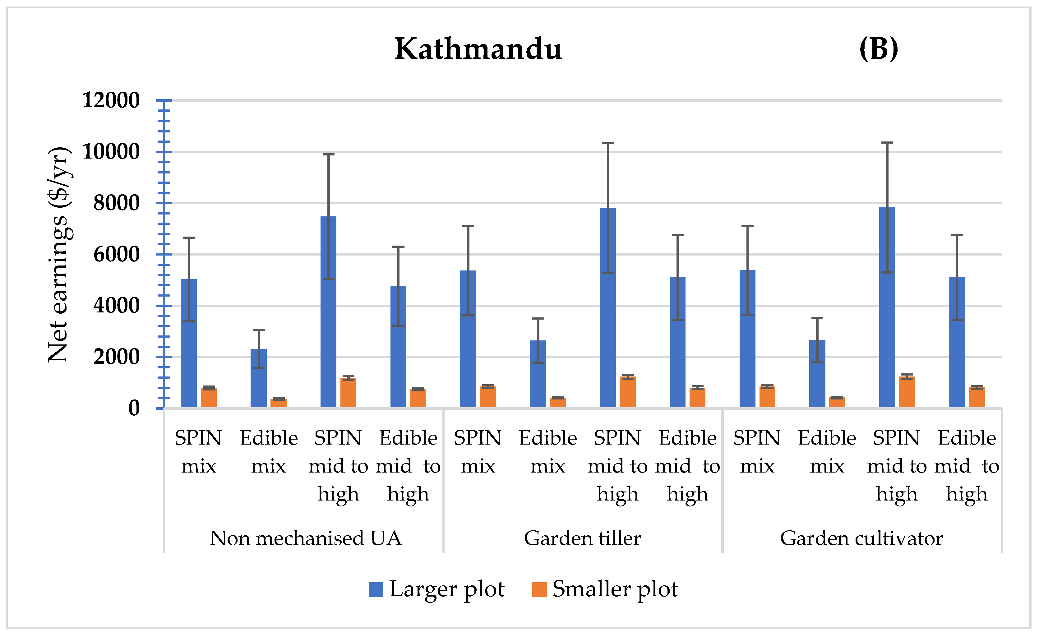
3.2. Net Earnings Calculation
3.3. Economy of Scale
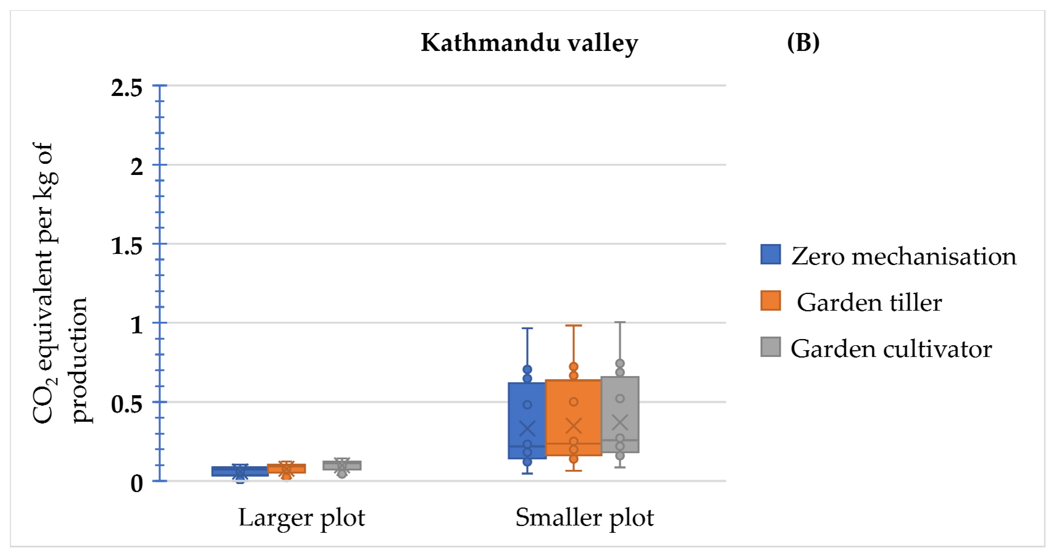
3.4. Carbon-Dioxide Emissions Calculation
3.4.1. Comparative Emission Analysis
Emissions from Fuel Use
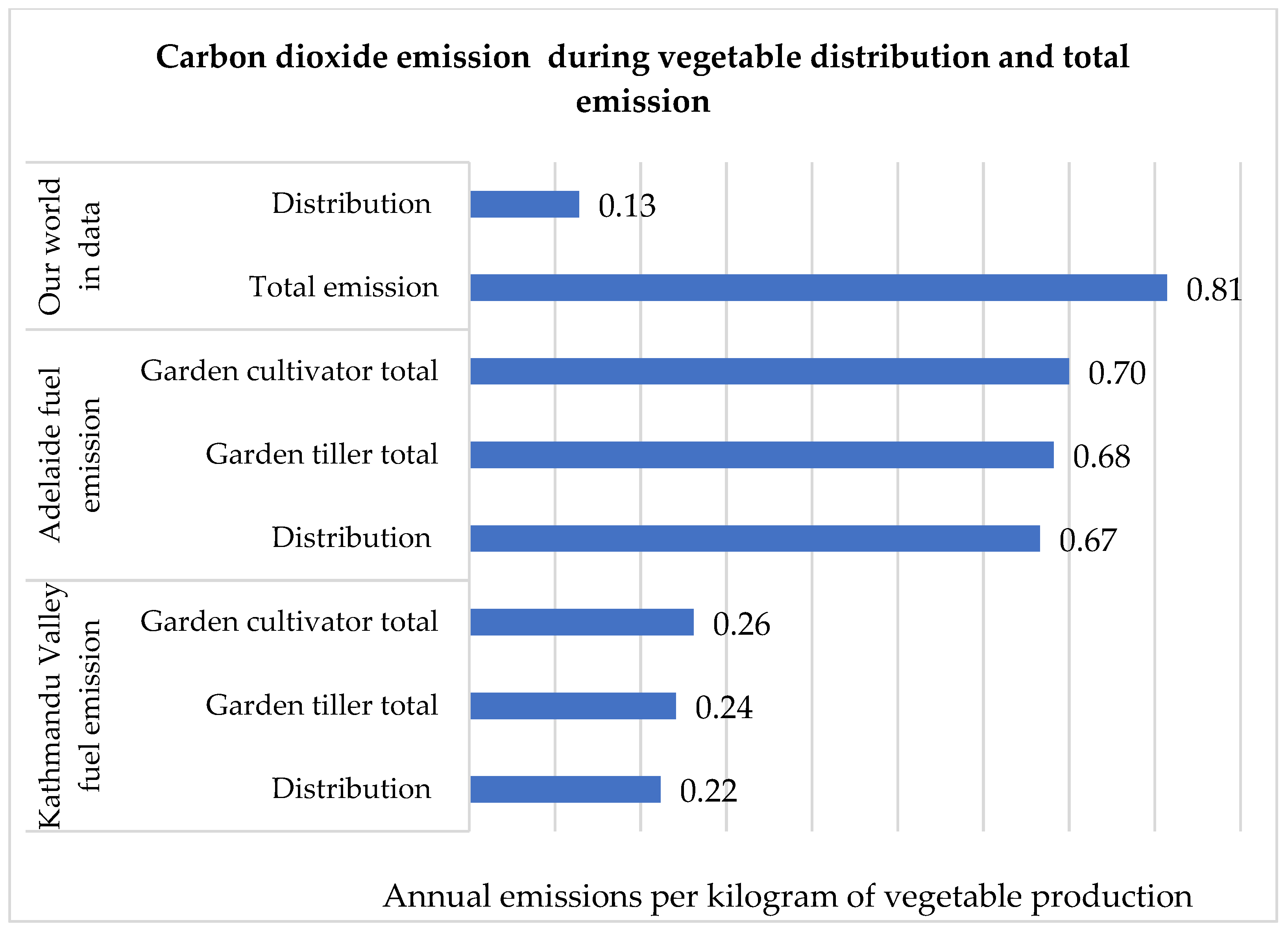
Distribution and Total Emissions
4. Discussion
4.1. Full-Time Employment Equivalent and Earnings
4.2. Economy of Scale
4.3. Carbon Dioxide Emissions
5. Conclusions
6. Policy Recommendations
- The advantage of mechanisation is dependent on labour costs; if it is a priority for governments to see wage growth, then mechanisation will become advantageous in the future as labour costs increase. Thus, the government could identify ways to support and promote sustainable small-scale mechanisation to improve the viability and sustainability of UA.
- There is considerable scope for improving the current distribution system for UA produce (e.g., shared modes and methods of transport, as well as more localised/decentralised markets), ultimately reducing larger emissions during distribution.
- Planners and policymakers may consider ways for subsidised labour arrangements, especially for high wage setting scenarios, improvement into the current UA production practices with less environmental footprints and production based on market value and demand for better economic viability.
Author Contributions
Funding
Data Availability Statement
Acknowledgments
Conflicts of Interest
References
- Dobbins, C.E.; Cox, C.K.; Edgar, L.D.; Graham, D.L.; Perez, A.G.P. Developing a Local Definition of Urban Agriculture: Context and Implications for a Rural State. J. Agric. Edu. Ext. 2020, 26, 351–364. [Google Scholar] [CrossRef]
- Game, I.; Primus, R. GSDR 2015 Brief: Urban Agriculture. 2015. Available online: https://sustainabledevelopment.un.org/content/documents/5764Urban%20Agriculture.pdf (accessed on 10 August 2022).
- Hakansson, I. Urban Sustainability Experiments in Their Socio-economic Milieux: A Quantitative Approach. J. Clean. Prod. 2019, 209, 515–527. [Google Scholar] [CrossRef]
- Sanye-Mengual, E.; Specht, K.; Krikser, T.; Vanni, C.; Pennisi, G.; Orsini, F. Social Acceptance and Perceived Ecosystem Services of Urban Agriculture in Southern Europe: The case of Bologna, Italy. PLoS ONE 2018, 13, e0200993. [Google Scholar] [CrossRef] [PubMed]
- Diekmann, L.O.; Gray, L.C.; Thai, C.L. More Than Food: The Social Benefits of Localised Urban Food Systems. Front. Sustain. Food Syst. 2020, 4, 534219. [Google Scholar] [CrossRef]
- O’Sullivan, C.A.; Bonnet, G.D.; McIntyre, C.L.; Hochman, Z.; Wasson, A.P. Strategies to Improve the Productivity, Product Diversity and Profitability of Urban Agriculture. Agric. Syst. 2019, 174, 133–144. [Google Scholar] [CrossRef]
- Dieleman, H. Urban Agriculture in Mexico City; Balancing Between Ecological, Economic, Social and Symbolic Value. J. Clean. Prod. 2016, 163, S156–S163. [Google Scholar] [CrossRef]
- Hallett, S.; Hoagland, L.; Toner, E. Urban Agriculture: Environmental, Economic and Social perspectives. In Horticultural Review; Wiley: Hoboken, NJ, USA, 2016; p. 44. [Google Scholar] [CrossRef]
- Rich, K.M.; Rich, M.; Dizyee, K. Participatory System Approach for Urban and Peri-urban Agriculture Planning: The Role of System Dynamics and Spatial Group Model Building. Agric. Syst. 2018, 160, 110–123. [Google Scholar] [CrossRef]
- Mason, D.; Knowd, I. The Emergence of Urban Agriculture Sydney, Australia. Int. J. Agric. Sust. 2010, 8, 62–71. [Google Scholar] [CrossRef]
- Martellozzo, F.; Landry, J.S.; Plouffe, D.; Soufert, V.; Rowhani, P.; Ramankutty, N. Urban Agriculture: A Global Analysis of the Space Constraints to Meet Urban Vegetable Demand. Environ. Rese. Lett. 2014, 9, 6. [Google Scholar] [CrossRef]
- Battaglia, M. Can Urban Agriculture Reduce Food Insecurity for the Urban Poor? The University of Sydney, Sydney Environment Institute: Sydney, Australia, 2018; Available online: https://sei.sydney.edu.au/opinion/can-urban-agriculture-reduce-food-insecurity-urban-poor/ (accessed on 24 March 2022).
- Grewal, S.S.; Grewal, P.S. Can Cities Become Self-reliant in Food? Cities 2012, 29, 1–11. [Google Scholar] [CrossRef]
- Tien, L.E.H.; Ly, V.T.H.; Han, C.N. The Role of Urban Agriculture for a Resilient City. J. Viet. Environ. 2020, 12, 148–154. [Google Scholar]
- Burton, P.; Lyons, K.; Richards, C.; Amati, M.; Rose, N.; Fours, L.D.; Pires, V.; Barclay, R. Urban Food Security, Urban Resilience and Climate Change; National Climate Change Adaptation Facility, Gold Coast. 2013. Available online: https://nccarf.edu.au/wp-content/uploads/2019/03/Burton_2013_Urban_food_security.pdf (accessed on 8 August 2022).
- Gulyas, E.Z.; Edmondson, J.L. Increasing City Resilience through Urban Agriculture: Challenges and Solutions in the Global North. Sustainability 2021, 13, 1465. [Google Scholar] [CrossRef]
- Glover, T.D.; Parry, D.C.; Shinew, K.J. Building Relationship, Accessing Resources: Mobilising Social Capital in Community Garden Contexts. J. Leis. Res. 2005, 37, 450–474. [Google Scholar] [CrossRef]
- Orsini, F.; Gasperi, D.; Marchetti, L.; Piovene, C.; Draghetti, S.; Ramazzotti, S. Exploring the Production Capacity of Rooftop Gardens (RTGs) in Urban Agriculture: The Potential Impact on Food and Nutrition Security, Biodiversity and Other Ecosystem Services in the City of Bologna. Food Sec. 2014, 6, 781–792. [Google Scholar] [CrossRef]
- Toranghi, C. Critical Geography of Urban Agriculture. Prog. Hum. Geogr. 2014, 38, 521–567. [Google Scholar] [CrossRef]
- Gray, L.; Elgert, L.; WinklerPrins, A. Theorising Urban Agriculture: North-South Convergence. Agric. Hum. Values 2020, 37, 869–883. [Google Scholar] [CrossRef]
- Hampwaye, G. Benefits of Urban Agriculture: Reality or Illusion? Geoforum 2013, 49, R7–R8. [Google Scholar] [CrossRef]
- Van Tuijl, E.; Hospers, G.J.; Vandenberg, L. Opportunities and Challenges of Urban Agriculture for Sustainable City Development. Eur. Spat. Res. Pol. 2018, 25, 2. [Google Scholar] [CrossRef]
- Lam, R. Scaling up Urban Agriculture for Emissions Reduction and Community Health. 2020. Available online: https://riskcenter.wharton.upenn.edu/studentclimaterisksolutions/scaling-up-urban-agriculture-2/ (accessed on 24 March 2022).
- Mancebo, K.W.; Liao, S.Z. The Application of Economic Value Added on Green Facilities of Urban Agriculture. 2018. Available online: https://www.e3s-conferences.org/articles/e3sconf/abs/2018/32/e3sconf_icsree2018_05001/e3sconf_icsree2018_05001html (accessed on 12 May 2022).
- Lovell, S.T. Multifunctional Urban Agriculture for Sustainable Land Use Planning in the United States. Sustainability 2010, 2, 2499–2522. [Google Scholar] [CrossRef]
- Benis, K.; Reinhart, C.; Ferro, P. Development of Simulation-based Decision Support Workflow for the Implementation of Building Integrated Agriculture (BIA) in Urban Context. J. Clean. Prod. 2017, 147, 589–602. [Google Scholar] [CrossRef]
- Pollard, G.; Roteman, P.; Ward, J.; Chiera, B.; Mantzioris, E. Beyond Productivity: Considering the Health, Social Value and Happiness of Home and Community Food Gardens. Urban Sci. 2018, 2, 97. [Google Scholar] [CrossRef]
- Nicholls, A.; Ely, A.; Birkin, L.; Basu, P.; Goulson, D. The Contribution of Small Scale Food Production in Urban Areas to the Sustainable Development Goals: A Review and Case study. Sustain. Sci. 2020, 15, 1585–1599. [Google Scholar] [CrossRef]
- Anzunre, A.G.; Amponsah, O.; Peprah, C.; Takyi, S.A. A Review of The Role of Urban Agriculture in the Sustainable City Discourse. Cities 2019, 93, 104–119. [Google Scholar] [CrossRef]
- Cohen, N.; Reynolds, K. Resource Needs for a Socially Just and Sustainable Urban Agriculture System: Lessons from the New York City. Renew. Agric. Food Syst. 2014, 30, 1–12. [Google Scholar] [CrossRef]
- Golden, S. Urban Agriculture Impacts: Social, Health, and Economic: A Litreature Review. University of California. 2013. Available online: https://ucanr.edu/sites/CEprogramevaluation/files/215003.pdf (accessed on 10 August 2022).
- Orsini, F.; Kahane, R.; Nono-Womdim, R.; Gianquinto, G. Urban Agriculture in the Developing World: A Review. Agron. Sustain. Dev. 2013, 33, 695–720. [Google Scholar] [CrossRef]
- Barthel, S.; Isendahl, C. Urban Gardens, Agriculture and Water Management: Sources of Resilience for Long Term Food Security in Cities. Ecol. Econ. 2013, 86, 224–234. [Google Scholar] [CrossRef]
- Lal, R. Home Gardening and Urban Agriculture for Advancing Food and Nutritional Security in Response to the COVID-19 Pandemic. Food Sec. 2020, 12, 871–876. [Google Scholar] [CrossRef]
- Andres, J.F. Can Urban Agriculture Become a Planning Strategy to Address Social-Ecological Justice? 2017. Available online: https://www.diva-portal.org/smash/get/diva2:1153064/FULLTEXT01.pdf (accessed on 8 March 2022).
- Ritchie, H.; Roser, M. Environmental Impacts of Food Production. 2020. Available online: https://ourworldindata.org/environmental-impacts-of-food (accessed on 20 July 2022).
- Dubbeling, M.; Van Veenhuizen, R.; Halliday, J. Urban Agriculture as a Climate Change and Disaster Risk Reduction Strategy. Field Actions Sci. Rep. J. 2019, 20, 32–39. [Google Scholar]
- Langemeyer, J.; Madrid-Lopej, K.; Beltran, A.M.; Mendez, G.V. Urban Agriculture-a Necessary Pathway Towards Urban Resilience and Global Sustainability? Lands Urban Plan. 2021, 210, 104055. [Google Scholar] [CrossRef]
- Zimmerer, K.S.; Bell, M.G.; Chirisa, I.; Duvall, C.S.; Egerer, M.; Hung, P.-Y.; Lerner, A.M.; Shackleton, C.; Ward, J.D.; Yacamán Ochoa, C. Grand Challenges in Urban Agriculture: Ecological and Social Approaches to Transformative Sustainability. Front. Sustain. Food Syst. 2021, 5, 668561. [Google Scholar] [CrossRef]
- Kafle, A.; Hopeward, J.; Myers, B. Exploring Conventional Economic Viability as a Potential Barrier to Scalable Urban Agriculture: Examples from two Divergent Development Contexts. Horticulturae 2022, 8, 691. [Google Scholar] [CrossRef]
- Dorward, A. Agricultural Labour Productivity, Food Prices and Sustainable Development Impacts and Indicators. Food Policy 2013, 39, 40–50. [Google Scholar] [CrossRef]
- Reimer, B. Farm Mechanisation: The Impact on Labour at the Level of the Farm Household. Can. J. Soc. 1984, 9, 429–443. [Google Scholar] [CrossRef]
- Hamilton, S.F.; Richards, T.J.; Shafran, A.P.; Vasilaky, K.N. Farm Labour Productivity and the Impact of Mechanisation. Am. J. Agric. Econ. 2020, 104, 1435–1459. [Google Scholar] [CrossRef]
- Aguilera, E.; Guzman, A.I.; Molina, M.G.D.; Soto, D.; Infante-Amate, A. From Animals to Machines: The Impact of Mechanisation on the Carbon Footprint of Traction in Spanish Agriculture: 1900–2014. J. Clean. Prod. 2019, 221, 295–305. [Google Scholar] [CrossRef]
- Paudel, G.P.; KC, D.B.; Rahut, D.B.; Khanal, N.P.; Justice, S.E.; McDonald, A. Smallholder Farmers’ Willingness to Pay for Scale-appropriate Farm Mechanization: Evidence from the Mid-hills of Nepal. Technol. Soc. 2019, 59, 101196. [Google Scholar] [CrossRef]
- Aryal, J.P.; Rahut, D.B.; Thapa, G.; Simtowe, F. Mechanisation of Small-scale Farms in South Asia: Empirical Evidence Derived from Farm households Survey. Tech. Soc. 2021, 65, 101591. [Google Scholar] [CrossRef]
- Vitterso, G.; Torjusen, H.; Laitala, K.; Tocco, B.; Biasini, B.; Csillang, P.; Duboys de Labarre, M.; Lecoeur, J.L.; Maj, A.; Malak-Rawlikowska, A.; et al. Short Food Supply Chains and Their Contribution to Sustainability: Participants View and Perceptions From 12 European Cases. Sustainability 2019, 11, 4800. [Google Scholar] [CrossRef]
- Kafle, A.; Myers, B.; Adhikari, R.; Adhikari, S.; Sanjel, P.K.; Padhyoti, Y. Urban Agriculture as a Wellbeing Approach and Policy Agenda for Nepal. In Agriculture, Natural Resources and Food Security; Timsina, J., Maraseni, T.N., Gauchan, D., Adhikari, J., Ohja, H., Eds.; Sustainable Development Goals Series; Springer: Cham, Switzerland, 2022; pp. 221–238. [Google Scholar] [CrossRef]
- Kulak, M.; Graves, A.; Chatterton, J. Reducing Greenhouse Gas Emissions with Urban Agriculture: A Life Cycle Assessment Perspective. Lands. Urban Plan. 2013, 11, 63–78. [Google Scholar] [CrossRef]
- Hume, I.V.; Summers, D.M.; Cavagnaro, T.R. Self-sufficiency Through Urban Agriculture: Nice Idea or Plausible Reality? Sustain. Cities Soc. 2021, 68, 102770. [Google Scholar] [CrossRef]
- Wise, P. Grow Your Own: The Potential Value and Impacts of Residential and Community Food Gardening; The Australia Institute: Canberra, ACT, Australia, 2014; Available online: https://www.tai.org.au/sites/default/files/PB%2059%20Grow%20Your%20Own.pdf (accessed on 1 July 2021).
- Timsina, N.P.; Poudel, D.P.; Upadhyaya, R.; Shrestha, A. Trend of Urban Growth in Nepal with a Focus in Kathmandu Valley: A Review of Processes and Drivers of Change. Tomor. Cities 2020. [Google Scholar] [CrossRef]
- Mitchell, M.; Iglesias, A.R. Urban Agriculture in Kathmandu as a Catalyst for Civic Inclusion of Migrants and the Making of a Greener City. Front. Archit. Res. 2019, 9, 169–190. [Google Scholar] [CrossRef]
- Satzewich, W.; Christensen, R. How to Grow Commercially on Under an Acre, Digging Deeper #1—Workflow; 2012; A guide to managing all the farming tasks of an owner operated farm. SPIN Farming Basics; Available online: https://spinfarming.com/product/dig-deeper-1-spin-farming-work-flow/ (accessed on 20 August 2017).
- Csortan, G.; Ward, J.; Roetman, P. Raw and partially-analysed data from the Edible Gardens Project based in South Australia; Housed at the University of South Australia, Mawson Lakes 5095, South Australia, Australia. 2020. Available online: https://data.unisa.edu.au/dap/DatasetResource.aspx?DatasetResourceID=2038&DatasetID=647219 (accessed on 15 August 2022).
- Eat for Health. Recommended Number of Serves for Adults. 2022. Available online: https://www.eatforhealth.gov.au/food-essentials/how-much-do-we-need-each-day/recommended-number-serves-adults (accessed on 10 March 2022).
- Ministry of Agriculture and Livestock Development. Statistical Information on Nepalese Agriculture; Government of Nepal, Ministry of Agriculture and Livestock Development, Statistics and Analysis Section: Kathmandu, Nepal, 2021. Available online: https://s3-ap-southeast-1.amazonaws.com/prod-gov-agriculture/server-assets/publication-1627186854094-8f369.pdf (accessed on 3 August 2021).
- Adelaide Central Market. Fruit and Vegetable. 2022. Available online: https://shop.adelaidecentralmarket.com.au/collections/fruit-vegetables?page=2 (accessed on 10 June 2022).
- Ramro, P. Kalimati Vegetable and Fruit Rate Today. 2022. Available online: https://ramropatro.com/vegetable (accessed on 10 June 2022).
- Safe Work SA. Minimum Wage. 2022. Available online: https://www.safework.sa.gov.au/workers/wages-and-conditions/minimum-wage (accessed on 24 August 2022).
- The Himalayan Times. Minimum Monthly Wage of Workers Raised 11 Percent to Rs 15,000. 2021. Available online: https://thehimalayantimes.com/business/minimum-montly-wage-of-workers-raised-11-per-cent-to-rs-15000 (accessed on 29 August 2021).
- Global Petrol Price. Gasoline Price, Litre. 2022. Available online: https://www.globalpetrolprices.com/ (accessed on 21 September 2022).
- Ecoscore. How to Calculate CO2 Emission from the Fuel Consumption? 2022. Available online: https://ecoscore.be/en/info/ecoscore/CO2 (accessed on 20 March 2022).
- Grafton power Products. Honda GX25 Mini 4-Stroke Engine. Available online: https://www.graftonpowerproducts.com.au/listing/honda-gx25-mini-4-stroke-engine/ (accessed on 15 July 2022).
- Horizontal Performance XR950. Petrol Multipurpose Engines. Available online: https://5.imimg.com/data5/YO/OG/XU/SELLER-1743276/petrol-multi-purpose-engines.pdf (accessed on 15 July 2022).
- Budget Direct. Fuel Consumption Survey. 2022. Available online: https://www.budgetdirect.com.au/car-insurance/research/average-fuel-consumption-australia.html (accessed on 24 August 2022).
- Paudel, P.; Sapkota, S.; Gyanwali, K.; Adhikari, B. Comparison of Vehicular Fuel Consumption and CO2 Emission Before and During the COVID-19 Pandemic in Kathmandu Valley. J. Innov. Eng. Educ. 2021, 4, 10–17. [Google Scholar]
- AUSVEG. Cost of Production of Australian Vegetable Growers; AUSVEG: Glen Iris, Australia, 2017; Available online: https://ausveg.com.au/app/uploads/2017/05/Costs-of-production-for-Australian-vegetable-growers-1.pdf (accessed on 2 August 2021).
- Maraseni, T.N.; Cockfield, G.; Maroulis, J.; Chen, G. An Assessment of Greenhouse Gas Emissions from the Australian Vegetables Industry. J. Environ. Sci. Health Part B 2010, 45, 578–588. [Google Scholar] [CrossRef]
- Poore, J.; Nemecek, T. Reducing Food’s Environmental Impacts Through Producers and Consumers. Science 2018, 360, 987–992. [Google Scholar] [CrossRef]
- Guo, L.; Song, Y.; Zhao, S.; Tang, M.; Guo, Y.; Su, M.; Li, H. Dynamic Linkage Between Aging, Mechanisations and Carbon Emissions from Agricultural Production. Int. J. Environ. Res. Public Health 2022, 19, 6191. [Google Scholar] [CrossRef]
- Liao, W.; Zeng, F.; Chanieabate, M. Mechanisation of Small-scale Agriculture in China: Lessons for Enhancing Smallholder Access to Agricultural Machinery. Sustainability 2022, 14, 7964. [Google Scholar] [CrossRef]
- Hu, Y.; Sun, J.; Zheng, J. Comparative Analysis of Carbon Footprint Between Conventional Smallholder Operation and Innovative Largescale Farming of Urban Agriculture in Beijing, China. PeerJ 2021, 9, e11632. [Google Scholar] [CrossRef]
- O’Halloran, N.; Fisher, P.; Rab, P. Options for Mitigating Greenhouse Gas Emissions from the Australian Vegetable Industry; Horticulture Australia Ltd., Sydney, NSW, Australia. 2008. Available online: https://www.daf.qld.gov.au/__data/assets/pdf_file/0008/69947/Hort-Fruit-Drought-Carbon-Report6.pdf (accessed on 8 August 2022).
- Venkat, K. Comparision of Twelve Organic and Conventional Farming Systems: A Life Cycle Greenhouse Gas Emissions Perspective. J. Sustain. Agric. 2012, 36, 620–649. [Google Scholar] [CrossRef]
- Ward, J.D.; Ward, P.J.; Mantzioris, E.; Saint, C. Optimising Diet Decisions and Urban Agriculture Using Linear Programming. Food Sec. 2014, 6, 701–718. [Google Scholar] [CrossRef]
- Maassen, A.; Galvin, M. How Urban Agriculture Can Hardwire Resilience into Our Cities. 2021. Available online: https://climatechampions.unfccc.int/how-urban-agriculture-can-hardwire-resilience-into-our-cities/ (accessed on 13 May 2022).
- Kiss, K.; Ruszkai, C.; Takacs-Gyorgy, K. Examination of Short Supply Chains Based on Circular Economy and Sustainability Aspects. Resource 2019, 8, 161. [Google Scholar] [CrossRef]
- Cronin, R.; Halog, A. A Unique Perspective of Materials, Practices and Structures Within the Food, Energy and Water Nexus of Australian Urban Alternative Food Networks. Circ. Econ. Sustain. 2022, 2, 327–349. [Google Scholar] [CrossRef]


Disclaimer/Publisher’s Note: The statements, opinions and data contained in all publications are solely those of the individual author(s) and contributor(s) and not of MDPI and/or the editor(s). MDPI and/or the editor(s) disclaim responsibility for any injury to people or property resulting from any ideas, methods, instructions or products referred to in the content. |
© 2023 by the authors. Licensee MDPI, Basel, Switzerland. This article is an open access article distributed under the terms and conditions of the Creative Commons Attribution (CC BY) license (https://creativecommons.org/licenses/by/4.0/).
Share and Cite
Kafle, A.; Hopeward, J.; Myers, B. Modelling the Benefits and Impacts of Urban Agriculture: Employment, Economy of Scale and Carbon Dioxide Emissions. Horticulturae 2023, 9, 67. https://doi.org/10.3390/horticulturae9010067
Kafle A, Hopeward J, Myers B. Modelling the Benefits and Impacts of Urban Agriculture: Employment, Economy of Scale and Carbon Dioxide Emissions. Horticulturae. 2023; 9(1):67. https://doi.org/10.3390/horticulturae9010067
Chicago/Turabian StyleKafle, Arun, James Hopeward, and Baden Myers. 2023. "Modelling the Benefits and Impacts of Urban Agriculture: Employment, Economy of Scale and Carbon Dioxide Emissions" Horticulturae 9, no. 1: 67. https://doi.org/10.3390/horticulturae9010067
APA StyleKafle, A., Hopeward, J., & Myers, B. (2023). Modelling the Benefits and Impacts of Urban Agriculture: Employment, Economy of Scale and Carbon Dioxide Emissions. Horticulturae, 9(1), 67. https://doi.org/10.3390/horticulturae9010067