Abstract
Environmental changes and the reduction in arable land have led to food security concerns around the world, particularly in urban settings. Hydroponic soilless growing methods deliver plant nutrients using water, conserving resources and can be constructed nearly anywhere. Hydroponic systems have several complex attributes that need to be managed, and this can be daunting for the layperson. Micro Indoor Smart Hydroponics (MISH) leverage Internet of Things (IoT) technology to manage the complexities of hydroponic techniques, for growing food at home for everyday citizens. Two prohibitive costs in the advancement of MISH systems are power consumption and equipment expense. Reducing cost through harvesting ambient light can potentially reduce power consumption but must be done accurately to sustain sufficient plant yields. Photosynthetic Active Radiation (PAR) meters are commercially used to measure only the light spectrum that plants use, but are expensive. This study presents Adaptalight, a MISH system that harvests ambient light using an inexpensive AS7265x IoT sensor to measure PAR. The system is built on commonly found IoT technology and a well-established architecture for MISH systems. Adpatalight was deployed in a real-world application in the living space of an apartment and experiments were carried out accordingly. A two-phase experiment was conducted over three months, each phase lasting 21 days. Phase one measured the IoT sensor’s capability to accurately measure PAR. Phase two measured the ability of the system to harvest ambient PAR light and produce sufficient yields, using the calibrated IoT sensor from phase one. The results showed that the Adaptalight system was successful in saving a significant amount of power, harvesting ambient PAR light and producing yields with no significant differences from the control. The amount of power savings would be potentially greater in a location with more ambient light. Additionally, the findings show that, when calibrated, the AS7265x sensor is well suited to accurately measure PAR light in MISH systems.
1. Introduction
The global increase in population [1] and rising urban migration [2] have drawn attention to food security risks around the world [3]. These pressing issues have been exacerbated by COVID-19 [4] and have led to an increased interest in home gardening [5,6,7,8]. Hydroponic systems are one method of home gardening that can fill this gap [9]. Hydroponic systems are ideal as they are resource efficient and do not require soil. Micro Indoor Smart Hydroponic (MISH) systems are small Internet of Things (IoT) appliances that range from the size of a closet to a small device that sits on a countertop. They automate the maintenance of the hydroponic growth process. MISH systems can be constructed at home with inexpensive IoT equipment [10,11] or are commercially available like the popular Aerogarden [12].
This study focuses on home constructed open-air MISH (MISH-O) systems. MISH-O systems expose plants to ambient light in addition to the artificial light the system provides. However, commercial MISH-O systems do not monitor the light that plants receive, thereby forgoing opportunities to conserve energy. Daylight harvesting, a technique widely used in greenhouses, modulates supplemental lighting based on sunlight [13]. To ensure that plants receive sufficient light, an expensive quantum meter is used to measure the Photosynthetic Active Radiation (PAR). Quantum sensors measure the photon flux of light in moles, most instruments represent this in µmol, per second, per m2 (µmols). These readings are used to modulate the lights without sacrificing crop yields [14]. The cost of PAR sensors is prohibitive, making it challenging for ordinary people to construct and develop efficient MISH-O systems at home.
The act of non-academic citizens conducting or assisting in scientific research has led to significant advancements in the field of ecology [15] and is known as citizen science. Citizen science is being used in to advance research in areas of Urban Agriculture (UA) to address food security [16,17,18,19]. Low-cost IoT equipment is successfully being used to facilitate participation in citizen science [20]. This study aims to enable citizen science through the development of cheap IoT MISH systems. Applying a citizen science approach, to the research and development of MISH, has the potential to assist in alleviating food insecurity. To facilitate this approach, research into inexpensive solutions for MISH-O systems is crucial. The most expensive IoT equipment needed in a daylight harvesting MISH-O system is the PAR meter. PAR meters are typically expensive and not practical for residential home gardeners to purchase—for example, the widely used Li-Cor 190 is approximately $500 and only available through commercial distributors.
Reducing the cost of PAR meters has been a goal for some time [21,22,23], but recent advancements [24,25,26] have been enabled through the advancement of cheap IoT sensors, microcontrollers, and data processing. Numerous studies have shown that these technologies’ capabilities are comparable to commercial sensors [24,25,26,27,28]. For example, Adhiwibawa and Kurniawan [27] measured the spectral values of paint pigments with a simple TSL250 photodiode and an Arduino. Their results showed a strong significant correlation of 0.98 with a lab-grade UV–Vis 1800 spectrophotometer.
Caya et al. [25] used an array of three VTB8440BH photodiode sensors and optical filters that only allowed 400 to 700 nm light. These diodes connected to an Arduino to read the sensors and the data were transferred to Raspberry Pi 2B. The array was compared to an Apogee SQ-420 for evaluation and was found to have a correlation of 0.98, with only a +/− 4.74% difference in the means [25]. This suggested that inexpensive IoT sensors can be used to measure PAR light. However, a not fully integrated IoT framework was used, and the data were simply stored and analysed later. With no IoT framework, the data cannot be integrated into a smart system. Additionally, the calibration, which was performed outdoors using direct natural sunlight, was done in a simple way by taking the highest raw value from the Apogee SQ-420 and dividing it by the highest raw value of the VTB8440BH. This was the only form of data processing used to calibrate the proposed sensor array [25]. As their sensor array was only tested with direct natural sunlight, it may struggle measuring PAR light from sources with different spectral qualities.
Kuhlgert et al. [24] developed a handheld open-source portable phenotyping device, used to capture the environmental conditions of cultivation, for example, PAR levels, humidity, and temperature. The system supports the idea of using inexpensive IoT equipment in the field. The system was built with a custom board using an Arduino base, that integrates several inexpensive sensors and cameras to record environmental data and upload it via Bluetooth to a nearby computer. It utilized a single TCS34715FN on the outer side of the device to measure PAR.
The TCS34715FN has a photodiode with multiple built-in filters that separate the light into Red, Green, and Blue sensor output channels. The RGB colours are combined in the microcontroller to produce a white light colour sensor output resulting in the combined output of RGBW. Similar to Caya et al. [25], the calibration used natural sunlight, but included a wider range of conditions. They included data from shaded areas as well as overcast days. The calibration was done using linear regression of the RGBW outputs against a Li-Cor 190R resulting in a correlation of 0.9967 and with a diffusion shield minimum of 0.9342. The calibrated sensor was deployed in multiple instantiations of the phenotyping device. The results were consistently accurate across all devices, demonstrating that an inexpensive sensor can accurately measure PAR and be integrated in functional IoT system.
Kutschera and Lamb [26], building on Kuhlgert et al. [24], built another Arduino based IoT device using the TCS34715FN to economically measure PAR. Similar to the PARduino [23], the device’s sole purpose was to measure PAR and display the readings; however, unlike Barnard et al. [23], there was no data logging capability. This was also the case with Kuhlgert et al. [24]. The sensor was covered with a half hemisphere white diffusion barrier. There was no calibration process, and the system employed the coefficients produced in Kuhlgert et al. [24]. The system was placed on the roof of a building with no obstructions. Data were collected over 72 h, comparing the system to a Li-Cor 190R, capturing data every 20 min. The results show a strong correlation and indicate no significant difference between the two PAR readings.
Both Kuhlgert et al. [24] and Kutschera and Lamb [26] focused on measuring sunlight. Kuhlgert et al. [24] used sunlight to produce the regression coefficients and provided a detailed account proving that the formula works well to predict PAR with sunlight on overcast days and at different heights compared to the plants canopy (meaning high, low, and in the middle). However, there was little information on how the PAR sensor was tested using artificial light, despite providing evidence that it worked with artificial light. Both Kuhlgert et al. [24] and Kutschera and Lamb [26] describe testing with violet LED and florescent tube lights, but this is only a fraction of the light wavelength required for plant growth.
The Kutschera and Lamb [26] study lack details of how the system was tested in artificial light. A single scatterplot chart shows the data points of “various white light sources” [26] (p. 2425) along with the regression formula results y = 0.5801x + 58.086. The correlation appears weaker when compared to the scatterplot charts for sunlight and overcast days. This suggests that the spectral composition of the artificial light sources are not the same as sunlight and thus the one set of coefficients calibrated from the sun will not be as accurate when used in a different setting as suggested by Nedbal et al. [29]. These points indicate that an inexpensive IoT sensor, calibrated using only sunlight, will struggle to accurately measure PAR light from a variety of sources.
Leon-Salas et al. [28] has used an AS7265x low-cost spectral sensor to create an alternative to an expensive PAR meter. This sensor system is different from the previous systems mentioned as it has three separate optical sensors combined on one board with a single I2C interface rather a single photodiode. Where the TCS34715FN provides four channel output (RGBW) [24,26], the AS7265x provides 18 channel output, with 20 nm spectral channels ranging from 410 to 940 nm. The system is similar to the design of the Kutschera and Lamb [26] using an Arduino and no datalogging capabilities. The data used for the calibration were a combination of LED light, fluorescent lamp light and solar light. The sensor was calibrated with a lab-grade Black Comet spectroradiometer. The raw values from the AS7265x were mapped using vector quantization to count µmols for each channel. This made the calculation of PAR easy by simply adding the µmols for each channel between the PAR spectrum up and arriving at the PAR equivalent. It was then tested under 10 different lighting conditions including various sunlight conditions and four different combinations of Red, Green, Blue, and White LED lights as well as a combination of sun and artificial light in a building atrium.
Incredibly, the inexpensive sensor, when trained with a lab-grade spectrometer, and adjusted for correction, outperformed the industry standard Li-Cor 190 quantum sensor [28]. It should be noted that the purpose of their sensor system was not integrated with any IoT system and shows great potential for measuring PAR economically in a MISH IoT system. The calibrated AS7265x and a Li-Cor 190R were compared against a spectroradiometer. The results showed that the trained AS7265x performed better than the Li-Cor 190R in every condition with a average error of 6.83 compared to 12.51 for the Li-Cor 190R [28].
Lork et al. [30] used a standard ISL29125 lux meter to measure PAR light with an unspecified method of calibration, likely a conversion formula. This is a common approach also used in all versions of MIT’s Food Computer [11,31]. There are a number of well-established conversion formulae available for lux [32]. However, these formulae only work with known spectral compositions [32]. This makes this sensor and approach for estimating PAR undesirable for our system as we are aiming to incorporate both sunlight and LED light combined.
The Lork et al. [30] system was classified as a MISH-C system and uses the Nutrient Film Technique (NFT), applying a film of nutrients to the roots of the plant with a stream of water. The system was built on a RPi 3 with an Arduino-based microcontroller and standard hydroponic system sensors attached: humidity, temperature, EC pH, as well as a camera. The system included image monitoring, a full data logging function, and a smart adapting light system that tracked the price of electricity and leaf size and adjusted the lighting based on these among other variables [30]. While it can be safely assumed that their PAR readings were not as accurate as other studies, they were still able to save money, by accounting for electricity price in their smart lighting algorithm and maintain acceptable biomass for their lettuce crop. This demonstrates potential for integrating an economical IoT sensor into a smart lighting MISH system despite a low level of accuracy measuring PAR.
The most relevant systems to our objective are those described by Jiang et al. [33] and Mohagheghi and Moallem [34]. Both present systems that use inexpensive sensors integrated into a smart lighting system, with the purpose of harvesting daylight to conserve resources. Daylight harvesting is a technique successfully used in both buildings and greenhouses to account for sunlight and adapt the lighting accordingly, providing a more efficient use resources [14,34,35,36,37]. Both Jiang et al. [33] and Mohagheghi and Moallem [34] utilize the TCS34725 light sensor to estimate PAR in their smart lighting systems.
Mohagheghi and Moallem [34] used the set points of the highest PAR value provided by the manufacturer, the wattage, and the values provided for the spectrum by Ryer [38] in their calibration formula. As with Lork et al. [30], there was no comparison to any quantum sensor or lab spectrometer to validate the accuracy of their PAR measurements. The experiment took place in a closed grow tent that used a centrally positioned halogen light to simulate sunlight and two red and blue spectrum grow lights positioned at a 45-degree angle on both sides of the plants. This system used the calibrated TCS34725 to dim the grow lights according to a given setpoint for DLI total. The system was only demonstrating the ability to provide dimmable supplemental red and blue light effectively. No plants were grown. The system was also not IoT integrated.
Finally, Jiang et al. [33] produced a MISH-O system that fully integrates the TCS34725 in a smart lighting system that harvests daylight to grow microgreens. The system uses a flood and drain hydroponic technique. The lighting that is provided uses two programmable (QuantoTech) luminaires composed of red and blue spectrum lights, building on Mohagheghi and Moallem [34]. Four TCS34725 sensors were used to measure the amount of red and blue ambient light, two near the window and two on the opposite side. Using Mohagheghi and Moallem’s [34] model, the readings were used to dim lights according to the minimum amount of desired supplemental light with reference to the incoming sunlight. In one experiment, they used desired set points from the raw readings of the TCS34725, rather than PAR, for both the red and blue spectrum. They then monitored ambient light and dimmed the red and blue light, in steps of 10%. In another experiment growing kale microgreens, they mapped these set points to the PAR reading of an Apogee MQ-501 and then estimated PAR and used this to modulate the red and blue lights. In both experiments, they achieved total energy savings between 34% and 21% [33]. When comparing the fresh weight of the control to that of the dimming system treatment, the adaptive light yield was slightly greater in fresh weight [33].
Jiang et al.’s [33] system is a full IoT smart system, implemented on a RPi. It uses a multiplexer to connect the multiple sensors on the I2C bus and an analog-to-digital converter for humidity and moisture sensors as well as a camera for canopy monitoring. The PAR meter is connected via USB serial and dimming is implemented on the LED controllers via a Wi-Fi connection. Data are fully logged and viewed through a dashboard on a browser. It is important to note that the dimming is not controlled directly by the system. The RPi sends a setting to the luminaires that dim accordingly in 10% steps. This leaves gaps in granularity of the dimming percentage and relies on the control of a separate external system to adjust the lights. Additionally, the calibration for the TCS34725 was not tested for accuracy with PAR, it is only assumed to be correct.
Over the years, the progress toward an inexpensive PAR meter has made significant strides with most recent work of Leon-Salas et al. [28] performing with greater accuracy than the Li-Cor 190R. Table 1 shows the low-cost sensors that have been used in the development of measuring PAR economically over the last five years. Of these studies, only two have applied their PAR light alternatives in an adaptive lighting system. As demonstrated in Table 1, there has been little work in exploring the application of these cheap methods of measuring PAR to harvest daylight through adaptive lighting for MISH systems. Out of the studies examined, the systems that developed the economical PAR measurement methods have not been integrated in full IoT systems. The systems that do use cheap sensors to estimate PAR in full IoT systems, use sensors that have limited abilities to capture the red spectrum for PAR, stopping at 615 nm [33,34]. Otherwise, they use sensors designed to measure luminous flux that focus on 555 nm range [30]. Additionally, Lork et al. [30] and Mohagheghi and Moallem [33] use standard techniques that convert various sensor inputs to PAR. While Lork et al. [30] use lux readings converted to PAR, Mohagheghi and Moallem [33] use watts. Both calibration formulae are dependent on knowing the specific spectral makeup of the light source for the formula to work. Additionally, the systems were not demonstrated in the environment in which a MISH system would actually be deployed. There is a clear gap for research into the area of an economical PAR sensor that can be applied into a full MISH-O system to harvest daylight in an actual real-world setting.

Table 1.
List of studies and the sensors that were used to develop low-cost PAR meters and/or, integrate them into an adaptive lighting system.
This study presents Adaptalight, a unique MISH-O system, building on the previous IoT MISH systems infrastructure and components. Adaptalight is a fully developed MISH-O system with a smart LED lighting system used to harvest daylight. Firstly, this study shows the suitability of the AS7265x as the choice sensor for economically measuring PAR and demonstrates the limitations of the TCS34725. Next, a calibrated AS7265x is integrated into the Adaptalight system to harvest ambient PAR light, similar to Jiang et al. [33]. However, to address the light modulation issues identified in Jiang et al.’s [33] system, Adaptalight uses a precise, direct pulse width modulation (PWM) control of the LED power source. Finally, this study evaluates the systems performance in a real-world setting, in an apartment in Dubai, UAE. The next section will present the system design used to construct the MISH-O system.
2. Materials and Methods
2.1. Adaptalight System Design
The system was constructed and deployed in an apartment living area. All system components were purchased locally. The system uses a flood and drain hydroponic technique. The flood table, 120 cm × 70 cm, was built to accommodate two 55 L trays from IKEA, that serve as flood tables. The nutrient reservoir is a 130 L IKEA storage tote that fills both 55 L trays using a Dymax 25-Watt 1200 L per hour water pump. The LED grow lights were locally sourced through Amazon.ae, each 300 mm × 240 mm with 110 W dimmable power supply. The LED spectral composition is 14 × 660 nm, 96 × 5000 k Samsung LM281B, 192 × 3000 k, 1 × 760 nm. The IoT system design is focused on the smart light aspect of MISH systems and therefore nutrient solution monitoring and plant growth monitoring are done manually. The database and dashboard servers were set up locally on services that could easily transition to identical services located in the cloud. For this study, they were kept locally to reduce cost.
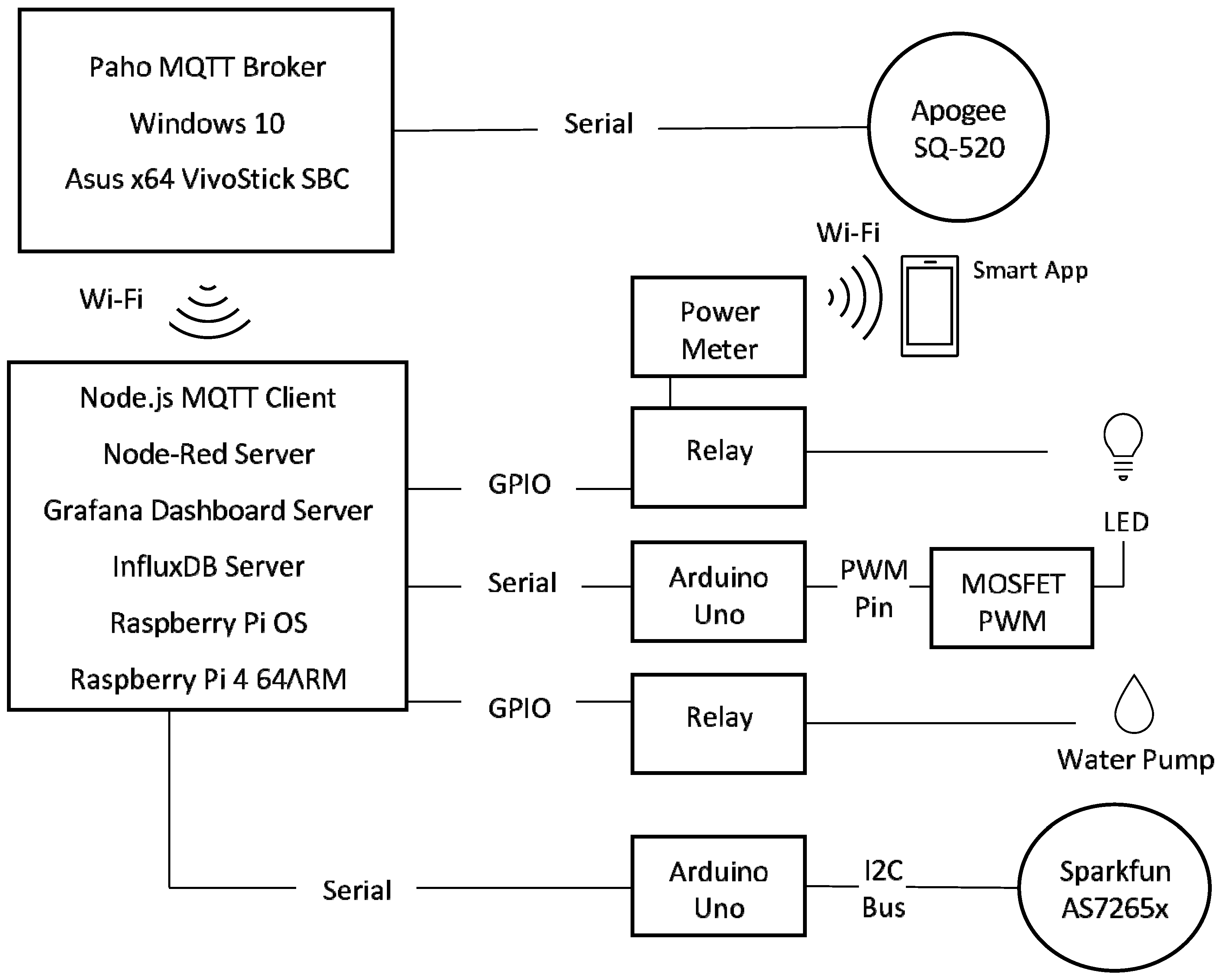
This study follows Peffers et al. [39] DSR Methodology, which has been iterated twice to improve the design of the system. The final resulting system architecture is shown in Figure 1. The first version incorporated the Adafruit TCS34725 [33,34]. After attempting calibration, the limitations of the sensor was evident and it was changed to the SparkFun AS7265x [28]. Incorporating this sensor changed the design as it needed a separate microcontroller. An Arduino Uno was added to read sensor data on the I2C bus. Initially, the Raspberry Pi 4 (RPi) was used for PWM. Unfortunately, the hardware created a noticeable pulse that was distracting to apartment residents. This was substituted with an Arduino Uno for greater reliability and finer granularity for light control. The AS7265x and PWM did not share the same microcontroller due to system data synchronization issues. MySQL was found too time consuming and was replaced with InfluxDB, a time series database more suited to IoT. Grafana, a dashboard service, was added to create the data monitoring system.

Figure 1.
Adaptalight architecture diagram—this shows the physical components as well as the services used to create the system.
2.2. Adaptalight IoT Architecture
As shown in Figure 1, the core of the system is a RPi that is running Raspberry Pi OS and Node-RED as the middleware. The RPi connects to a local area network using standard Wi-Fi. It has a statically assigned IP address making it easily locatable. It has three different services available at the same IP address with different TCP port numbers, Node-Red 1880, Grafana 3000, InfluxDB 8888. GPIO pins connect two relays that are actuated with Node.js libraries. These relays control the water pump and the LED luminaires. USB serial connections communicate with two Arduino Uno’s, using a built-in Node.JS library. The Node-RED MQTT client was used to receive MQTT packets over Wi-Fi to integrate the Apogee SQ-520 sensor into the system.
The Apogee SQ-520 was used to measure PAR in the system, similar versions of this sensor were used in Jiang et al. [33] and Mohagheghi and Moallem [34]. Due to regional availability constraints, this was used instead of the Li-Cor190. The Apogee SQ-520 connects via USB and can only be read with a Windows software, Apogee Connect. An Asus VivoStick TS10 x64 SBC was used to run Apogee Connect and read the sensor data. Python was used to build a software that creates a MQTT broker and send. The Asus VivoStick connects via the Wi-Fi LAN to send the MQTT packets to the RPi [40].
Two Arduino Unos are used in the system connected via Node-RED’s serial library. One Arduino connects the AS7265x on I2C bus and reads data every 10 s. Another Arduino is used to control the dimming of the LED with a MOSFET connected to the Arduino analogue PWM pin. The PWM modulation uses the default 8 bits to adjust the voltage with values between 0 and 255. This gives direct control of the brightness levels and greater granularity than Jiang et al. [33].
The LED light and the pump are connected to relays that are controlled through Node-RED RPi GPIO pin library (Figure 1). Node-RED scheduling libraries are used to actuate the relays according to user settings. To measure the power of the LED lights, a Broadlink BestCon SCB1 was placed inline. These data were not integrated into the database and was collected separately through a mobile app that provided both hourly and daily readings.
2.3. Adaptalight Software System Design
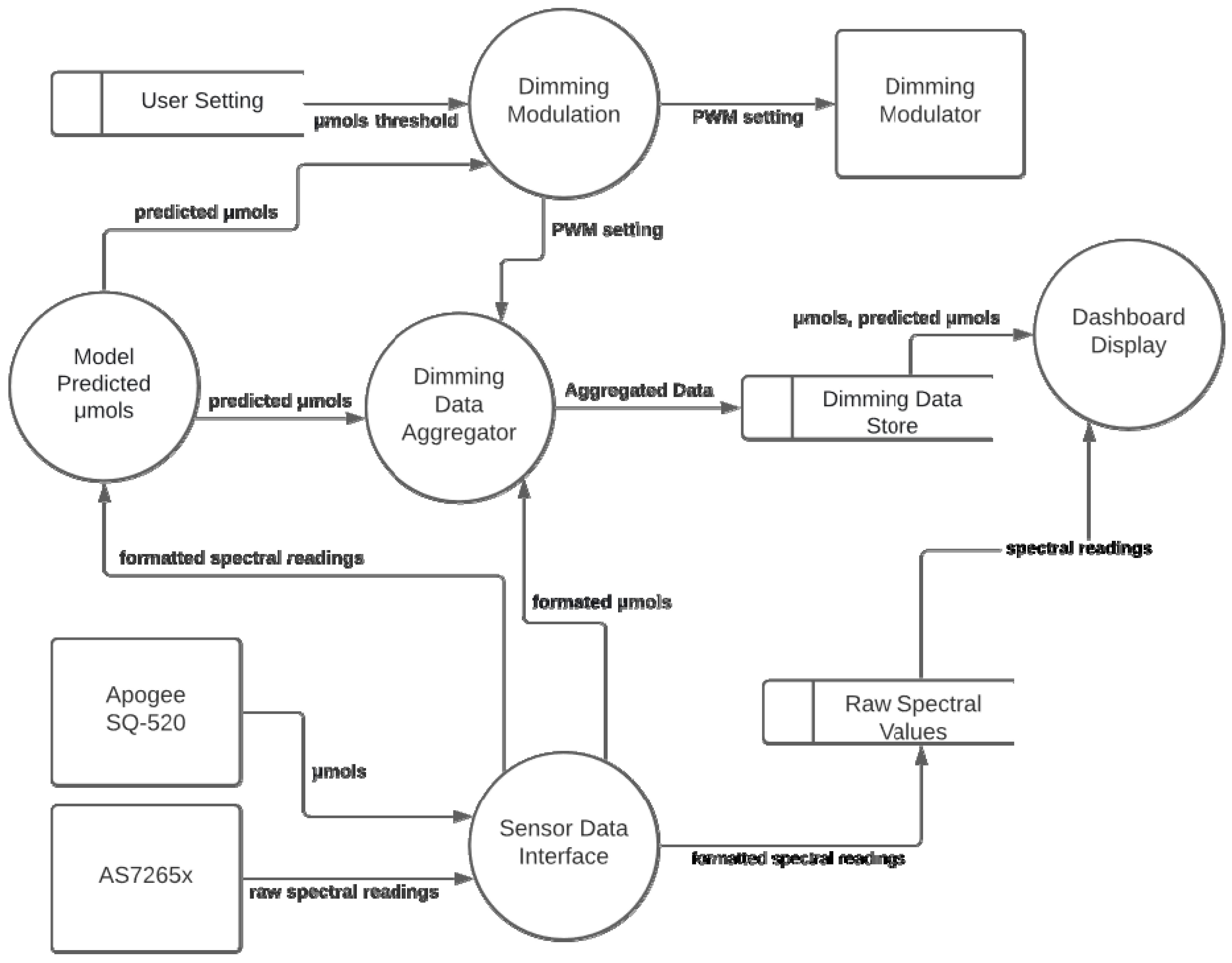
The Adaptalight system, in Figure 2, is made of five processes and three data stores. The system compares the real-time μmols to the desired user threshold. The user setting, stored in μmols, are stored directly in the database. To change the threshold, the database needs to be updated directly. In Figure 2, the sensor data from Apogee SQ-520 are referred to as μmols. The AS7265x provides 18 spectral channels readings, referred to in Figure 2 as the raw spectral readings.

Figure 2.
Data flow diagram of the Adaptalight system.
The sensor data interface creates three JSON objects from the data. The μmols and raw spectral readings are combined and sent with a timestamp to InfluxDB. Storing this data together eases access for analysis tools and populating the dashboard. The model predicted μmols process, in Figure 2, runs data through a trained model deployed in the standard multiple linear equation below.
P = A + C1 × X1 + … + C18 × X18
In the equation P is the predicted μmols, which is the result of adding A, the alpha intercept, to the product of C, the coefficient, and X, the raw spectral reading. There are 18 sets of corresponding spectral channels and coefficients that are used in calculating the predicted µmols. The predicted µmols is forwarded to the dimming data aggregator, and to the dimming modulation process.
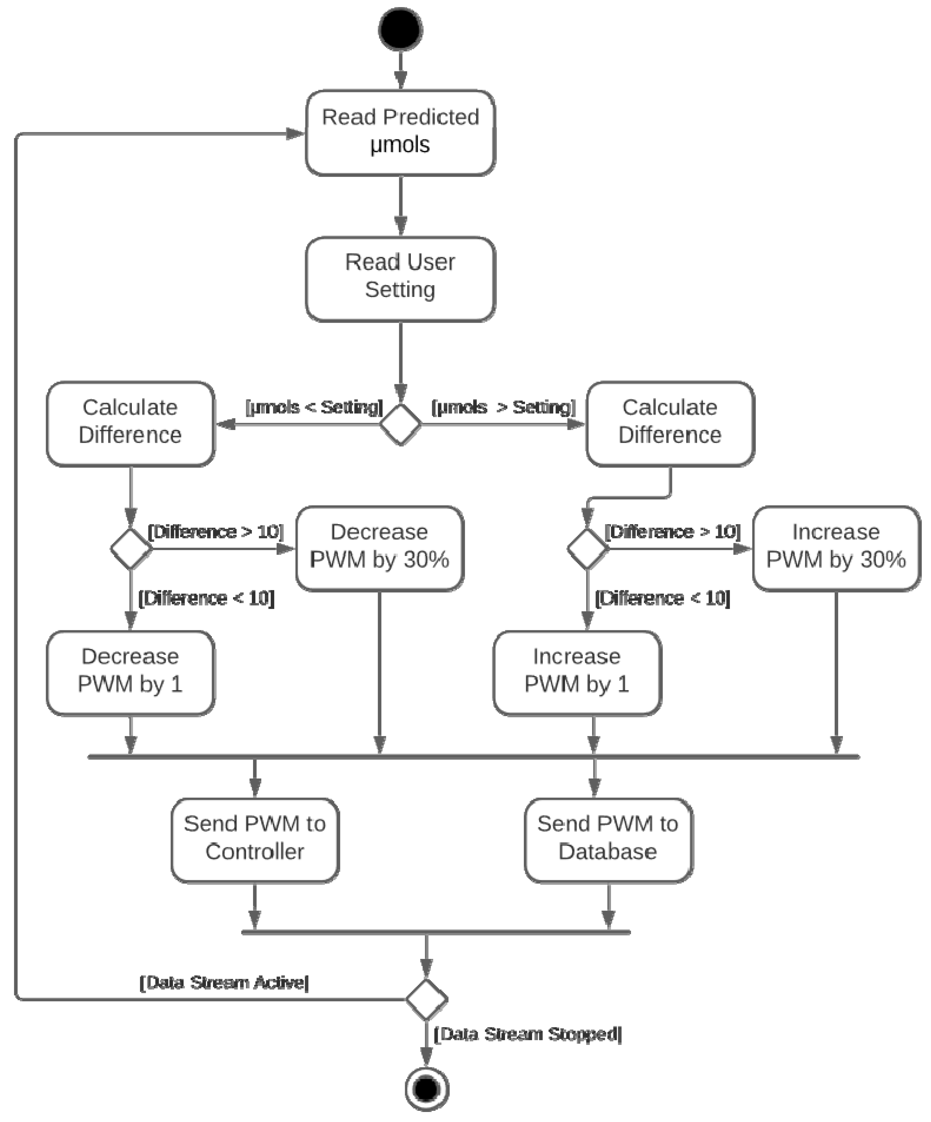
Dimming modulation uses the algorithm in Figure 3 to compare the predicted μmols to user setting μmols threshold. This will generate a PWM setting integer, which the dimming modulator uses to dim the lights accordingly. Finally, in Figure 2, the dimming data aggregator combines three JSON objects, the current PWM setting, the predicted μmols, and the μmols readings from the Apogee SQ-520. These are aggregated with a single timestamp to eliminate time drift, then sent to an InfluxDB table in the dimming data store.

Figure 3.
Dimming algorithm used in the PWM controller.
The dashboard display process, in Figure 2, uses Grafana to issue queries to the both the dimming data store and the raw spectral values to create an easy to monitor user interfaces pulling together all the data generated from the lighting system in one place.
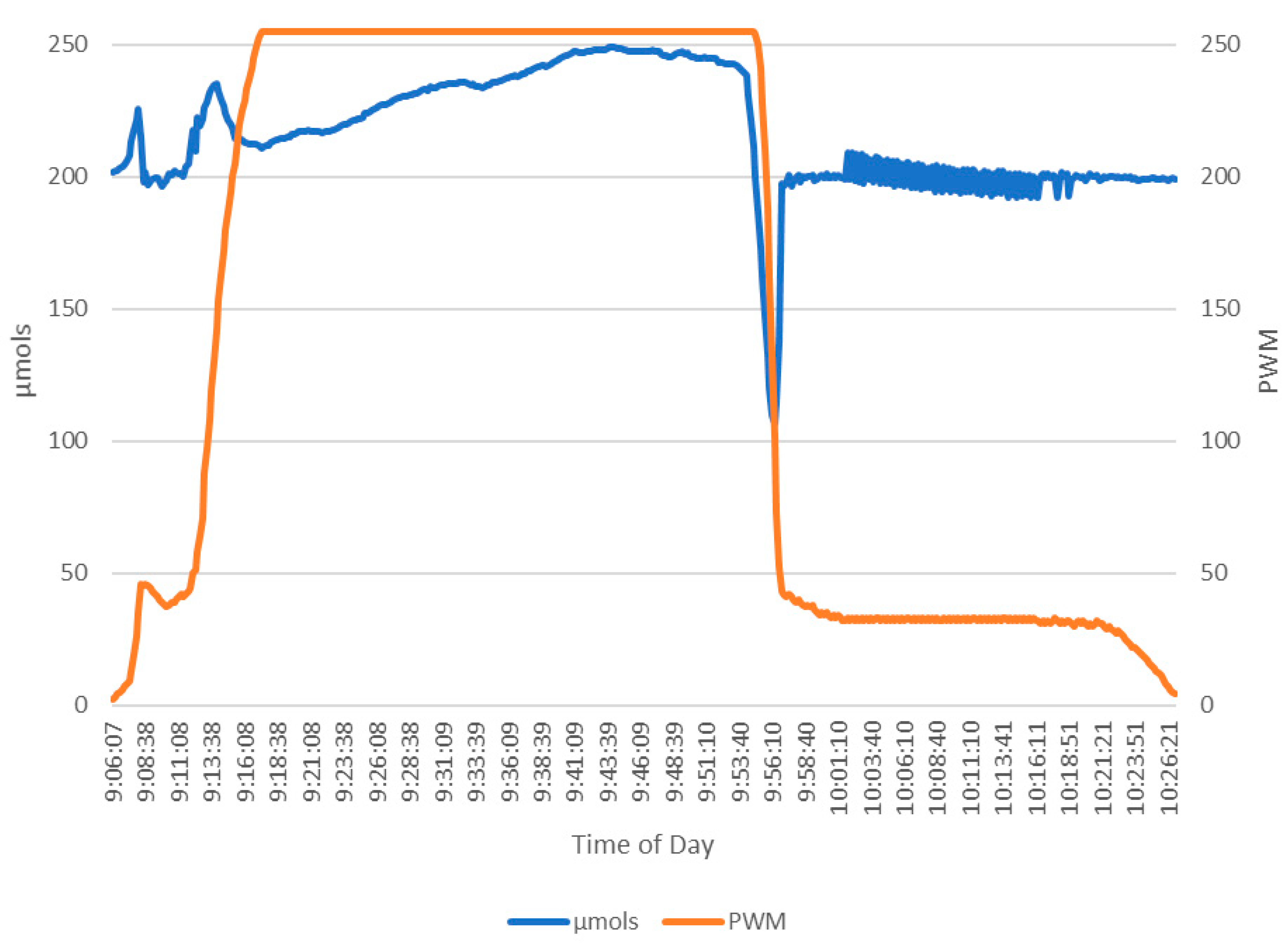
To evaluate the effectiveness of the dimming algorithm in Figure 3, the Apogee SQ-520 data were routed to the dimming modulation process in place of the predicted µmols. The user setting was set to 200 µmols. As expected, with an increase above 200 µmols, the PWM increases accordingly, causing the LED lights to dim. The dimming algorithm in Figure 3, is the second iteration. A 30% adjustment was added because the system processes data in 10 s intervals but adjusting the PWM by one step every 10 s did not provide the sufficient responsiveness in the first iteration. The effectiveness of the 30% PWM adjustment, in Figure 3, is clear. In Figure 4, the sunlight increases and the PWM signal closely tracks the sunlight. When the sudden spike of sunlight occurs at 09:07, the system quickly tracks moving from 9 PWM to 45 PWM. Again, when the sunlight finally drops at 09:55, within 60 s the PWM stabilizes at 162 and continues tracking. In testing, the PWM and µmols have a strong significant correlation (r(450) = 0.71, p < 0.001), successfully demonstrating the system and algorithm’s control abilities.
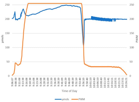
Figure 4.
Evaluating the Adaptalight dimming algorithm. The times shown are when the most ambient light comes into the system. The desired setting or 200 µmols was used. When PWM increases, the lights dim.
2.4. Sensor Evaluation
This section discusses the evaluation of two sensors and the suitability of linear modelling for calibration. The evaluation for each followed a three-step process. First, data were collected for model building, next the best model was selected, and finally the model was deployed for performance evaluation in the Adaptalight system.
2.4.1. Evaluating TCS34725 Sensor
First, a calibration approach for the TCS34725 was selected. Jiang et al. [33] and Mohagheghi and Moallem [34] both use this sensor but do not fully report methods for building a calibration model. Jiang et al. [33] used a mapping process while Mohagheghi and Moallem [34] uses an opaque calibration formula not readily available. Therefore, a linear modelling technique was selected based on Kuhlgert et al.’s [24] successful work with a similar sensor TCS34715N. To derive the standard linear model format Y = A + Bx. The Apogee SQ-520 µmols served as the dependent variable and TCS34725 as the independent predictors.
Three different models were constructed with different data sets. The sensor was mounted in the assigned location of the system near the window, collecting sensor readings every 30 s. The window faces eastward toward the courtyard on the first floor. Direct sun was present in the morning for around 120 min a day. Model 1, in line with Kuhlgert et al. [24], was built using only sunlight data recorded over 12 days. Model 2, in line with Jiang et al. [33], was constructed incorporating LED light in the data set over 15 days and used three permutations: exclusively LED light, exclusively sunlight, and a combination of LED and sunlight. Model 3 used a curated version of Model 2 data set. It included two of each value, for all permutations, covering the entire range. Based on the R2 and Mean Squared Error (MSE) in Table 2 Model 1 and Model 3 were selected for evaluation. The goodness of fit shows that Model 1 is the best. Model 3 was also evaluated based on Jiang et al.’s [33] success while using a model that incorporated the LED light in the calibration.
Table 2.
Goodness of fit matrix for TCS34725 calibration Models 1, 2 and 3. All models were significant with a p ≤ 0.000.
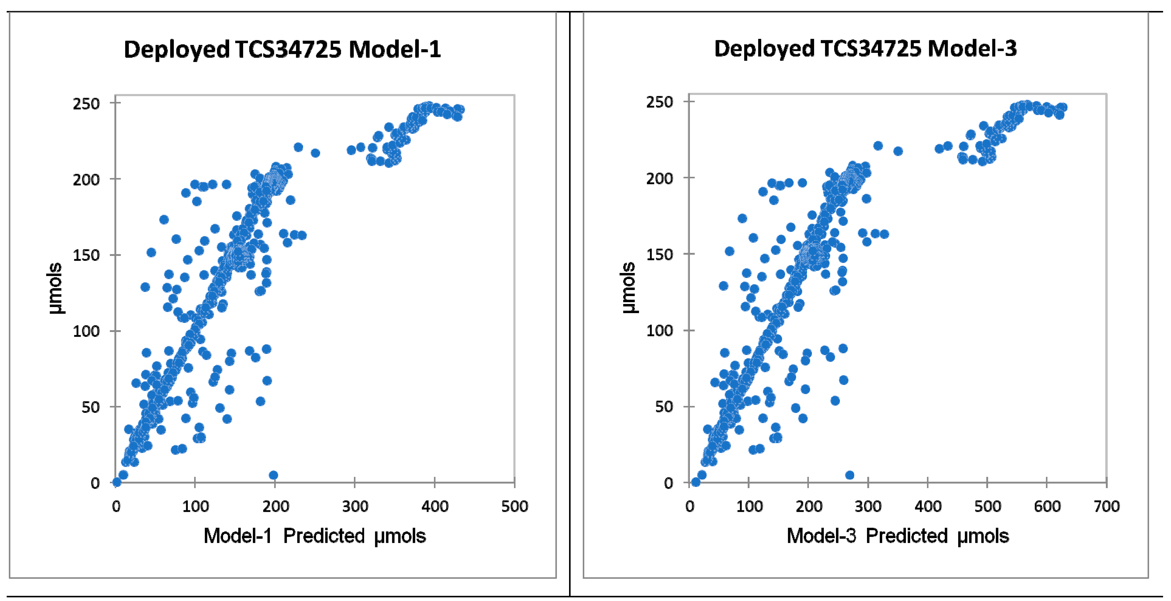
Model 1 and Model 3 were deployed during the evaluation of the PWM dimming algorithm discussed in Section 2.3. Observing the system’s response over 48 h showed that both Model 1 and Model 3 had issues predicting µmols to an acceptable level. Figure 5 shows clear evidence of a strong significant correlation. However, there is a clear gap where the sensor cannot perform. In Figure 5, the same performance gap can be seen for Model 1 and Model 3 despite different light intensities, exposing the sensor’s limitation. This will not work to dim lights accurately.
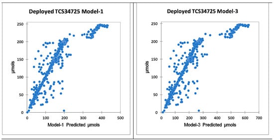
Figure 5.
These show the correlation of the deployed models over a 48 h period during the PWM dimming evaluation experiment. Model 1 had a correlation of 0.911 and Model 3 had a correlation of 0.886, both with p < 0.00.
Based on this analysis, the TCS34725 is not suitable to use in any setting for sensing PAR light. This is further supported by the limitation of the red LED spectrum for the TCS34725. It only measures up to 615 nm, while PAR goes to 700 nm. This sensor should be avoided when measuring PAR light. The Sparkfun AS7265x has a wider spectrum and accurate results as shown by Leon-Salas et al. [28].
2.4.2. Evaluating AS7265x Sensor
The AS7265x has three optical sensors, and each sensor has six channels. Each channel is 20 nm in width and covers the spectrum from 410 to 940 nm. Calibration data were captured over five days, in 30 s intervals, using the same combinations of light as Model 3. Two linear regression models were constructed using the Y = A + Bx. Model 4 using all 18 channels as coefficients and Model 5 using only 12 channels in the PAR spectrum. The Apogee SQ-520 was used for the dependent variable in the Y value, in units of µmols, and each of the channels served as the independent variable in X value. Based on the goodness of fit statistics in Table 3, Model 4 was selected for deployment evaluation, Appendix D shows the B coefficients for the model. These preliminary findings suggest an advantage using all 18 channels. This is in line with a previous study that used all 18 channels to measure PAR Leon-Salas et al. [28].
Table 3.
Goodness of fit matrix for AS7265x calibration Models 4 and 5. All models were significant with a p ≤ 0.000.
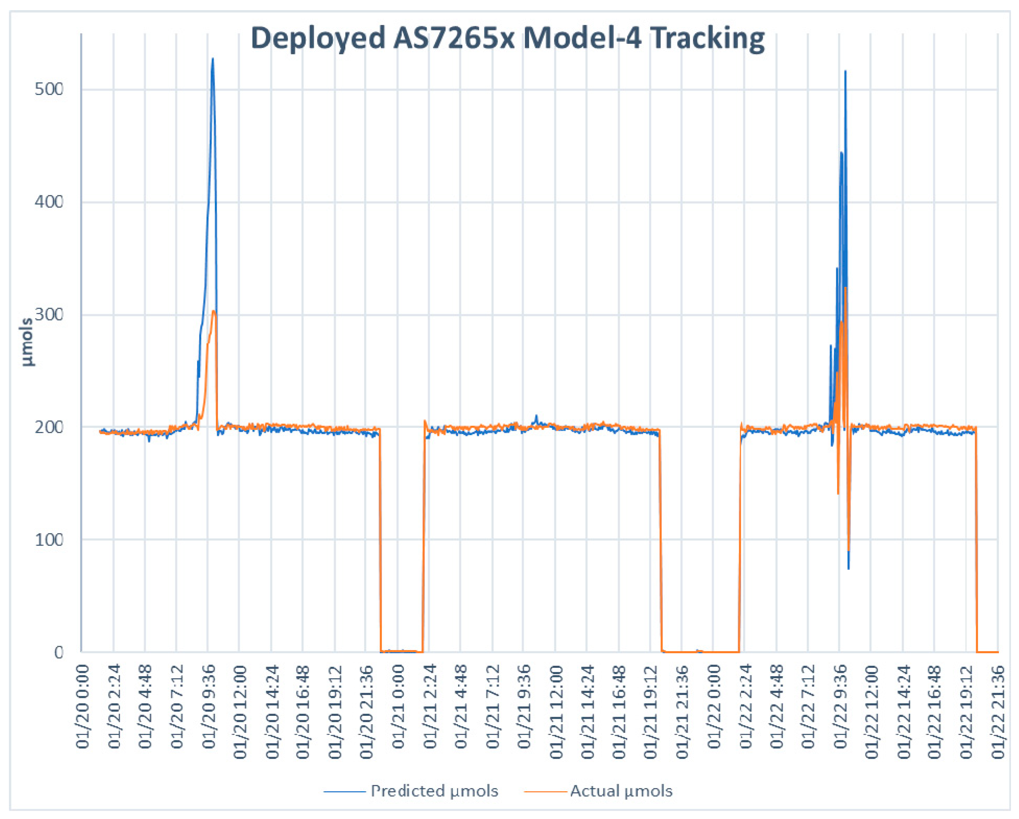
Model 4 was deployed for five days using the same settings used for performance evaluation of the TCS34725. Figure 6 shows the strong significant correlation (r(14,319) = 0.962, p < 0.000) between the predicted values of the AS7265x and the Apogee SQ-520. Figure 7 shows a dashboard tracking the predicted µmols against the actual µmols over three days. To demonstrate consistency, the date range selected included an overcast day, 21 January 2021. While there are some extreme outliers for the predicted µmols in both Figure 6 and Figure 7, overall, the pattern shows a sensitivity that responds in the same manner as the Apogee SQ-520. These findings are in line with Leon-Salas et al. [28] and combine as strong evidence for this method of model building and show that the sensor is well suited to be deployed in the system.
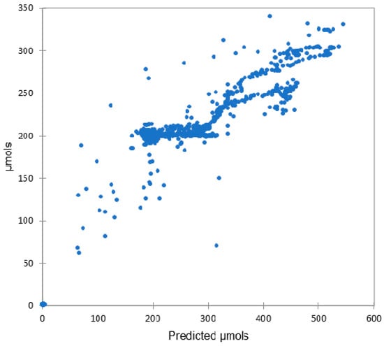
Figure 6.
Evaluation of AS7265x using Model 4, shown as predicted µmols correlated with Apogee SQ-520, shown as µmols. The results were a strong correlation of 0.964 with a p < 0.000.
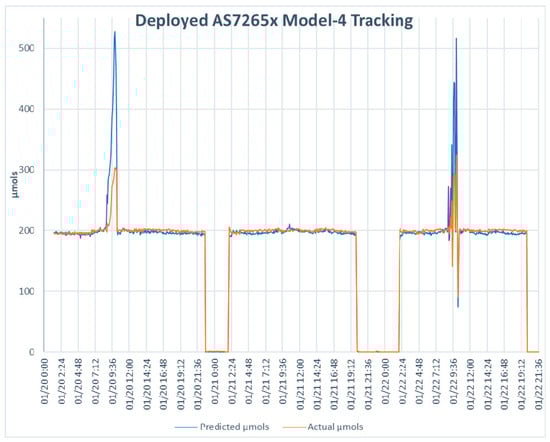
Figure 7.
The deployed AS7265x with Model 4 tracked against the µmols readings of the Apogee SQ-520 over the three days of the sensor evaluation. Note, 21 January 2021 was an overcast day.
After this evaluation, the AS7265x was permanently mounted to conduct the two-phase experiment shown in Figure 8. Once the sensor was permanently relocated, Model 4 no longer worked. The sensor produced extremely inaccurate predictions, leading to the conclusion that the sensor must be placed where it is to be mounted, then data must be collected to build the model. Only then will the sensor be able to accurately predict µmols using linear modelling. The next section presents the methodology used to conduct the two-phase experiment.
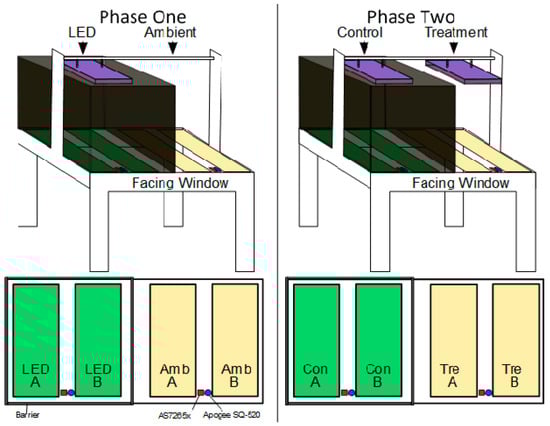
Figure 8.
Phase one shows the system setup for comparing the two sensors, trays are denoted with A and B in each chamber. Phase two shows the system setup for implementing Adaptalight light system on the ambient chamber. The LED chamber uses a barrier to block ambient light. The sensor placement is at the edge to best capture the ambient light.
2.5. Adaptalight Experiment Methodology
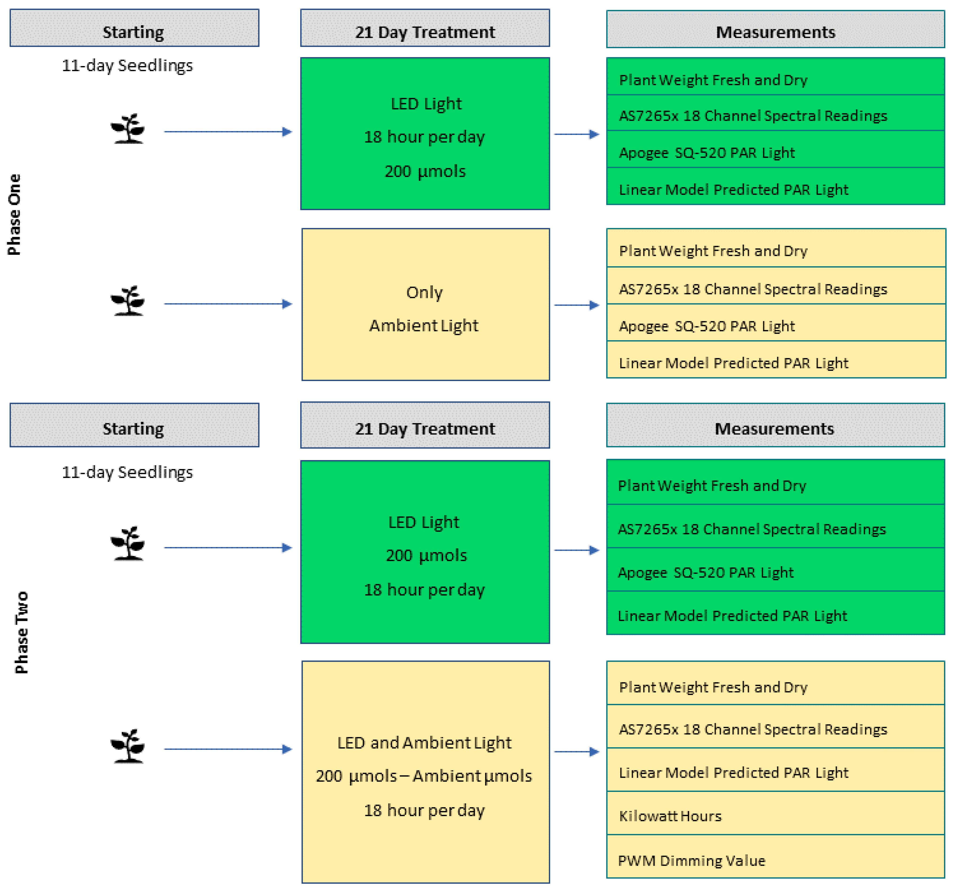
This section presents the methods for the experiments carried out in the evaluation phase of the Design Science Research Methodology (DRSM). This was a two-phase experiment as shown in Figure 8 and Figure 9. During system testing, it was demonstrated that the Adaptalight smart lighting system works well with an industrial-grade PAR sensor. The next step was to tune the system and replace the industrial sensor with the inexpensive IoT sensor. This was done through a two-phase experiment. Phase one examined the ability of the calibrated AS7265x to accurately measure PAR light compared with the Apogee SQ-520, and served as control for phase two, while identifying adjustments. The second phase used the calibrated AS7265x implemented in the Adaptalight MISH system to harvest ambient light. Both phases are conducted on the apparatus described in Section 2.1. Shown in Figure 8, the flood table is placed facing the only window to allow ambient light to come into the system.
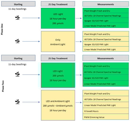
Figure 9.
This shows two treatments and the measurements collected for the operationalised variables. PAR light indicates the Apogee SQ-520 sensor, and the predicted PAR light is the calibrated AS7265x, both measured in µmols. The spectral readings are the raw values of the AS7265x 18 spectral channels of the. Phase two is similar to phase one, with notable exceptions. Only the calibrated AS7265x is used to measure PAR light on both sides. The measurement of kilowatt hours is added as is the PWM dimming signal sent to the lights.
Lettuce (Lactuca sativa) was selected for both phases of the experiment. It is a thoroughly researched crop for hydroponic systems and evaluating lighting [13,41,42,43,44]. Grow specification were from Brechner et al. [45] Frequency of flooding the benches was once every 12 h. The nutrient electrical conductivity (EC) was maintained at 1150–1250 above the baseline EC of the water. The pH was maintained at a level between 5.6 and 6.0. EC and pH were monitored daily. The nutrient solution is a locally available commercial-grade A/B solution. A standard aquarium solution was used to adjust pH. Each growth was started with 11-day-old seedlings and lasted 21 days in the system (Figure 9). Every 2 days, the Apogee SQ-520 was alternately moved between the control and experimental chambers. On day 10, trays A and B, in Figure 8, swapped places, to ensure even coverage. On day 21, the plants were harvested and dried in an oven for 72 h.
Phase one, seedlings were transplanted into the grow trays. The height of grow light was adjusted so all the plants received 200 µmols at the edge of the tray resulting in 230 µmols at the centre. A photoperiod of 18 h to meet the recommended daily light integral (DLI) for lettuce was set to maintain DLI of 14 [46,47,48]. A functional DLI was chosen, which can easily be used as a threshold for dimming. Using 200 µmols also allows the system more sensitivity to ambient light.
Phase two added a LED grow light to the ambient light side, with the same specifications from phase one including height and photoperiod settings. The ambient side grow light was connected to the Adaptalight modulation system. Both the lights were connected to a smart meter to track the amount of kilowatt hours. The lighting modulation system was set to monitor the ambient light coming into system and dim the grow lights accordingly. A minimum threshold of 200 µmols was set. When ambient light caused readings to exceed 200 µmols, the grow lights were dimmed accordingly.
Due to regional product availability and time constraints, only one Apogee SQ-520 was procured. Because of this, the sensor was alternated between chambers during the experiment rather than having one for each side. Since the experiments were conducted in a real-world application, the quality of ambient light varied from day to day depending on the cloud cover and air quality index of Dubai. The sensor placement was oriented to optimally capture the ambient light coming through the window. Because the LED light is predictable, the focus was optimally on measuring the light entering the window. Additionally, due to availability and time constraints, only two AS7265x were procured.
3. Results
This section presents the findings for both phases of the Adaptalight system experiments carried out between 18 March and 9 May 2021. The results are organized by sensor results, plant growth results, and power consumption results.
3.1. Sensor Results
A new linear model was created after mounting the sensors. Data were captured for both the ambient and LED chambers, shown in Figure 8, for five days. This was used to construct the prediction models used in phase one. It is important to note that no light modulation was carried out in phase one, only the observation of the models’ performance and plant growth. Appendix A shows the goodness of fit statistics and the coefficients used for both sides. The ambient model (R2 = 88.7 MSE = 56.945) was less accurate than the LED (R2 = 99.8 MSE = 22.78).
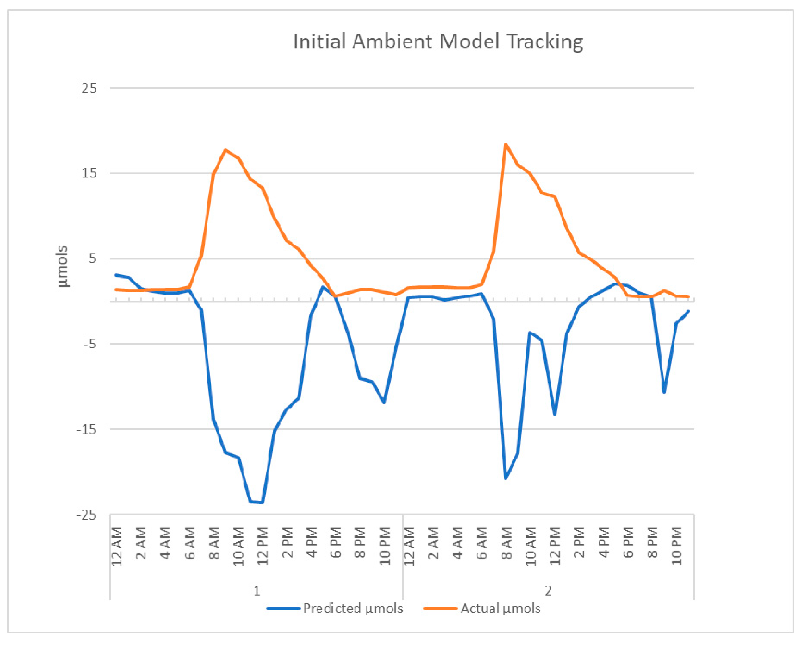
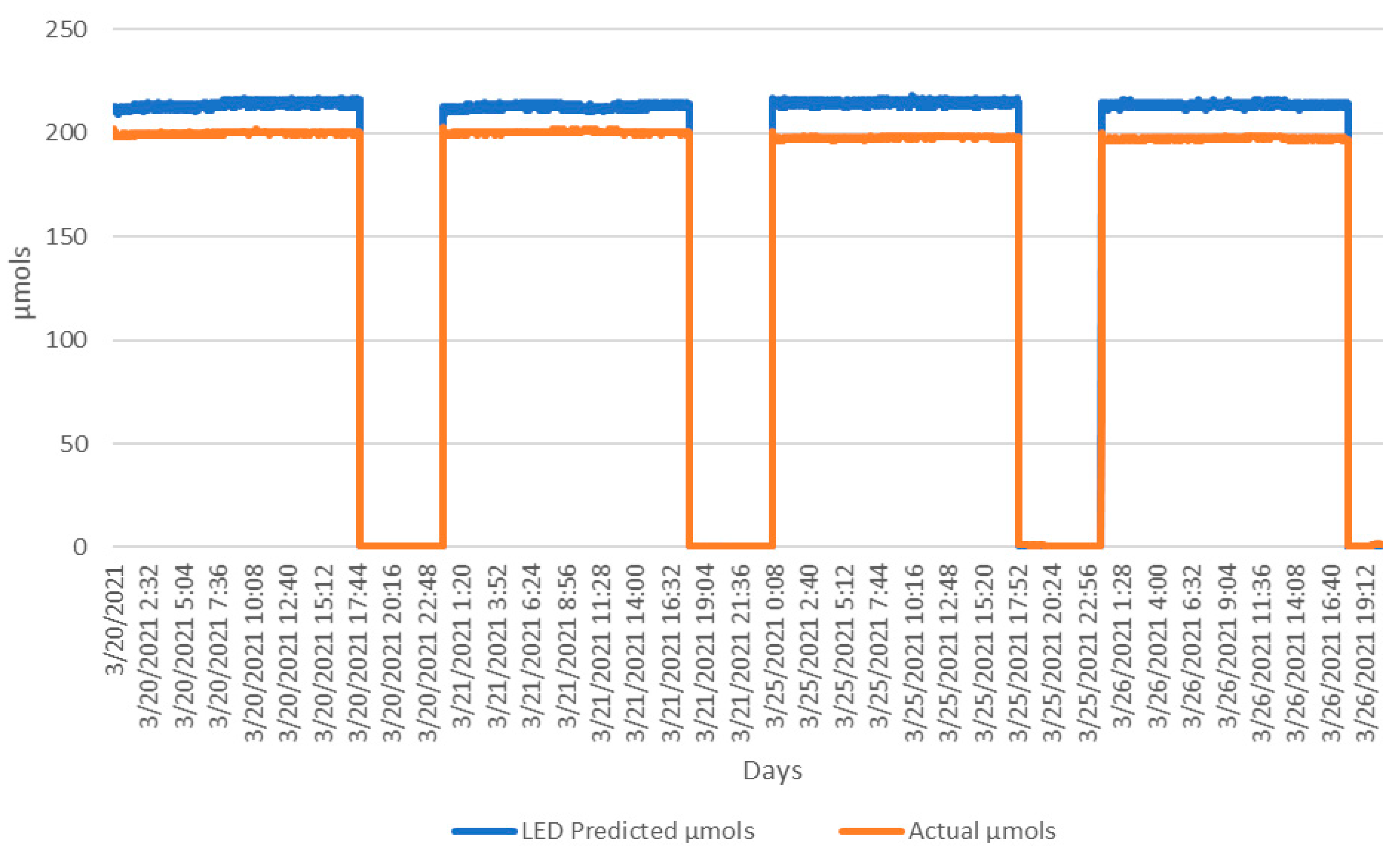
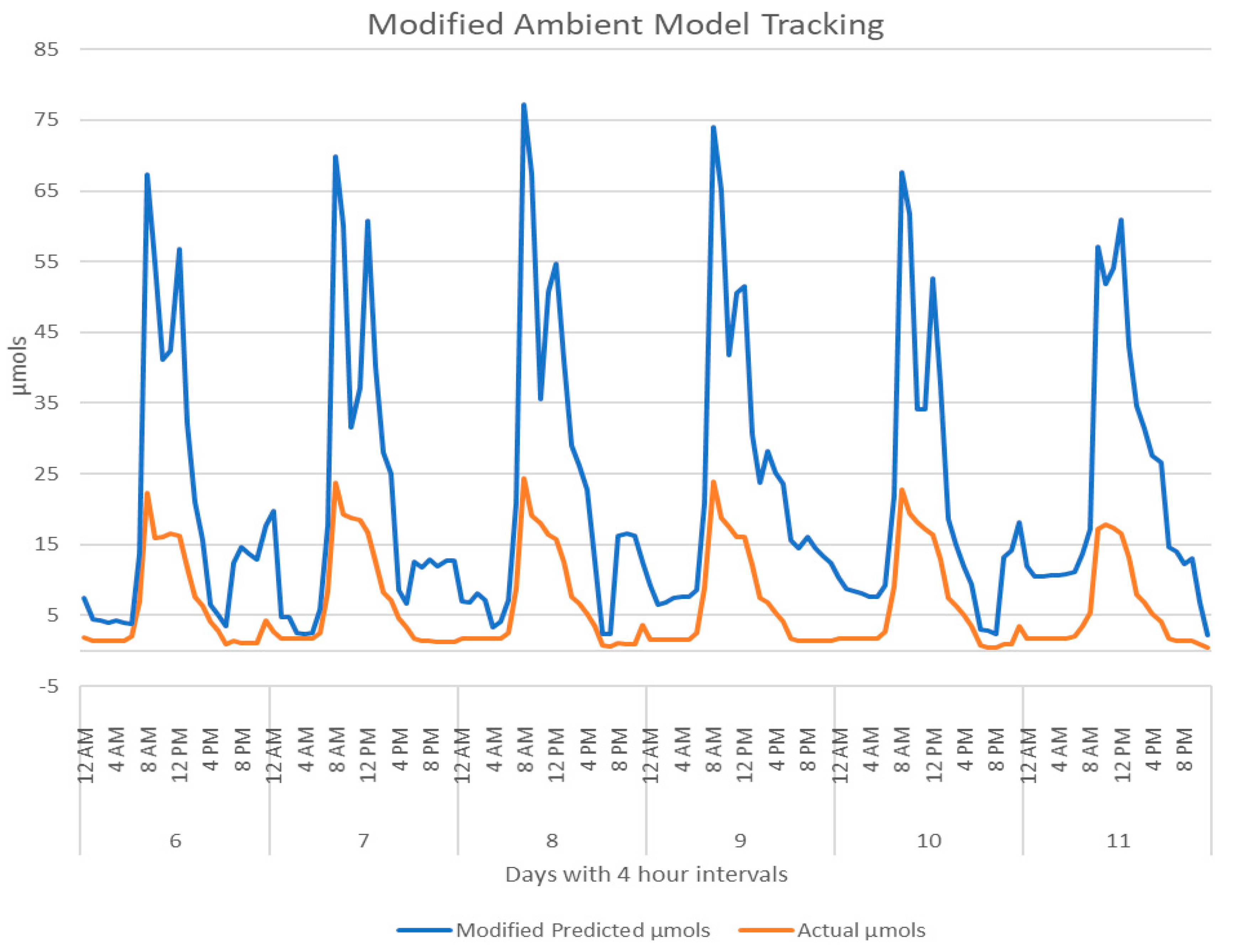
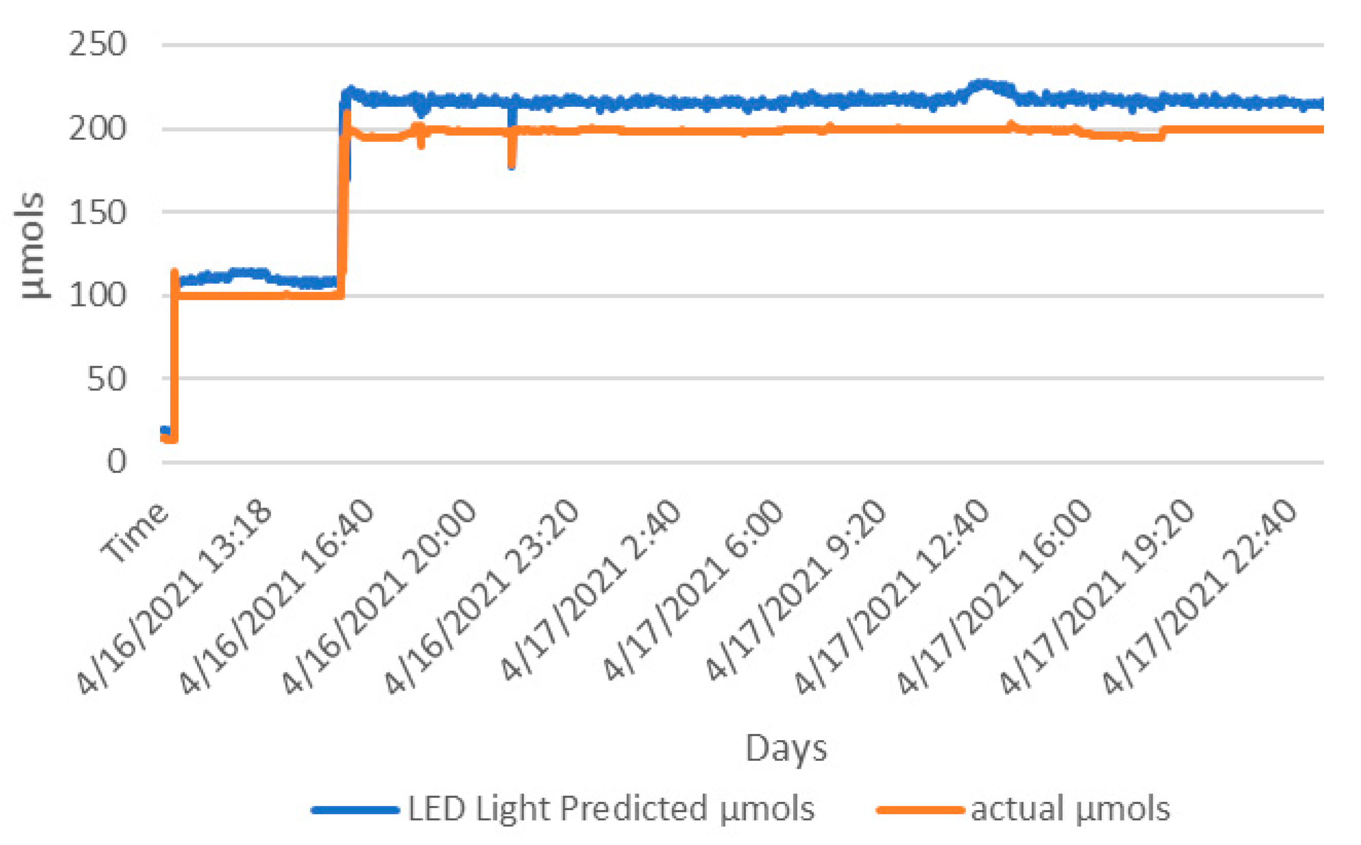
Figure 10 shows the AS7265x with the phase-one LED light model tracking against the Apogee SQ-520. The light was calibrated with only the LED spectral values and consistently reported a small percentage over the actual values. The initial deployment of the phase-one ambient model, in Appendix B, immediately flagged an issue and corrective measures were taken. The model produced the inverse predictions of the actual µmols. A simple inversion modification was created with a negative factor of one. Figure 11 shows the tracking for the ambient light model after the adjustment was made.
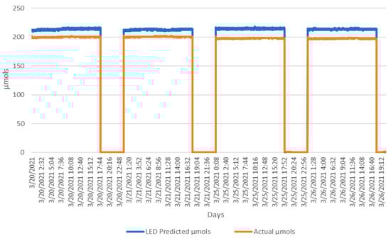
Figure 10.
The four days of the deployed LED light model predicting µmols against the actual µmols values.
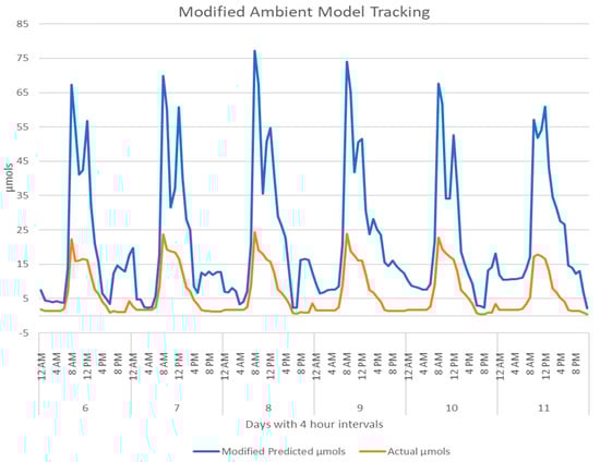
Figure 11.
The modified calibration results for the AS7265x in the ambient chamber compared to the Apogee SQ-520 for days six to 11.
For phase-one results, the mean PAR light values of the calibrated AS7265x on the LED light treatment side (M = 152.90, SD = 98.48) was 19.24 µmols greater than the actual µmols from the Apogee SQ-520 (M = 133.65, SD = 86.60). This small but significant difference (t(63,358) = 1.96, p < 0.001), supports the capability of the AS7265x of measuring PAR light consistently. Similar results are demonstrated on the ambient side. The PAR light values of the calibrated AS7265x with modifier (M = 11.92, SD = 12.36) were 5.96 µmols greater when compared to the actual µmols (M = 5.96, SD = 7.06). This significant difference (t(63,198) = 1.96, p < 0.001) is in line with the LED light chamber and further supports the calibrated AS7265x.
Tracking models in Figure 10 and Figure 11 show both calibrated sensor deployments align closely to the commercial PAR sensor readings. As expected, based on the R2 and MSE results of the linear modelling, the phase-one LED model performed better than the phase-one ambient model. A Pearson’s Correlation was used to test the relationships between the sensors. There was a significantly strong positive correlation (r(63,358) = 0.988, p< 0.001) between the calibrated AS726x on the LED light side and the Apogee SQ-520. On the ambient light side, the calibrated AS7265x also showed a significant strong positive correlation with the Apogee SQ-520 (r(63,198) = 0.726, p < 0.001), although slightly less. These two correlation statistics, along with the significant results of the t tests, strongly support the use of a calibrated AS7265x in place of a commercial PAR meter for measuring PAR light.
The LED model of phase one performed well and was deployed in phase two. To validate the model and check for adjustments, prior to deployment, 30 h of LED data were captured. The LED light was set to 100 µmols for six hours and then 200 µmols for 24 h shown as in Figure 12. The significant difference of means (t(2338) = 1.96, p < 0.001) showed the predicted model (M = 199.678, SD = 41.742) was 8% greater than the actual µmols values (M = 182.792, SD = 38.624) of the Apogee SQ-520. This difference was considered and a reduction of 8% was applied to the LED model from phase one and then deployed to both chambers of phase two, as shown in Figure 8.
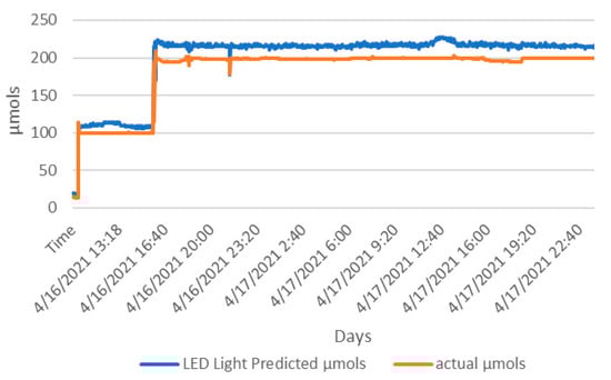
Figure 12.
Deploying the phase-one LED model to the ambient side sensor for 30 h for calibration. The Apogee SQ-520 is shown as actual µmols and the AS7265x with phase-one LED model is the LED light predicted µmols.
As expected, over the course of the 21 day experiment, the calibrated sensor in phase two performed similar to phase one. The mean of the treatment chamber’s AS7265x (M = 149.71, SD = 86.15) with the calibrated adjustment was 12.88 µmols significantly greater (t(43,796) = 1.96, p < 0.001) than the Apogee SQ-520 (M = 136.829, SD = 86.468). Compared to the control side the AS7265x (M = 182.979, SD = 104.242), with no adjustment, had a significantly greater mean of 33.56 µmols (t(63,358) = 1.96, p < 0.001) than the Apogee SQ520 (M = 149.410, SD = 85.023). This demonstrates the effectiveness of the calibration adjustment and further supports the use of the AS7265x sensor in place of a commercial PAR sensor.
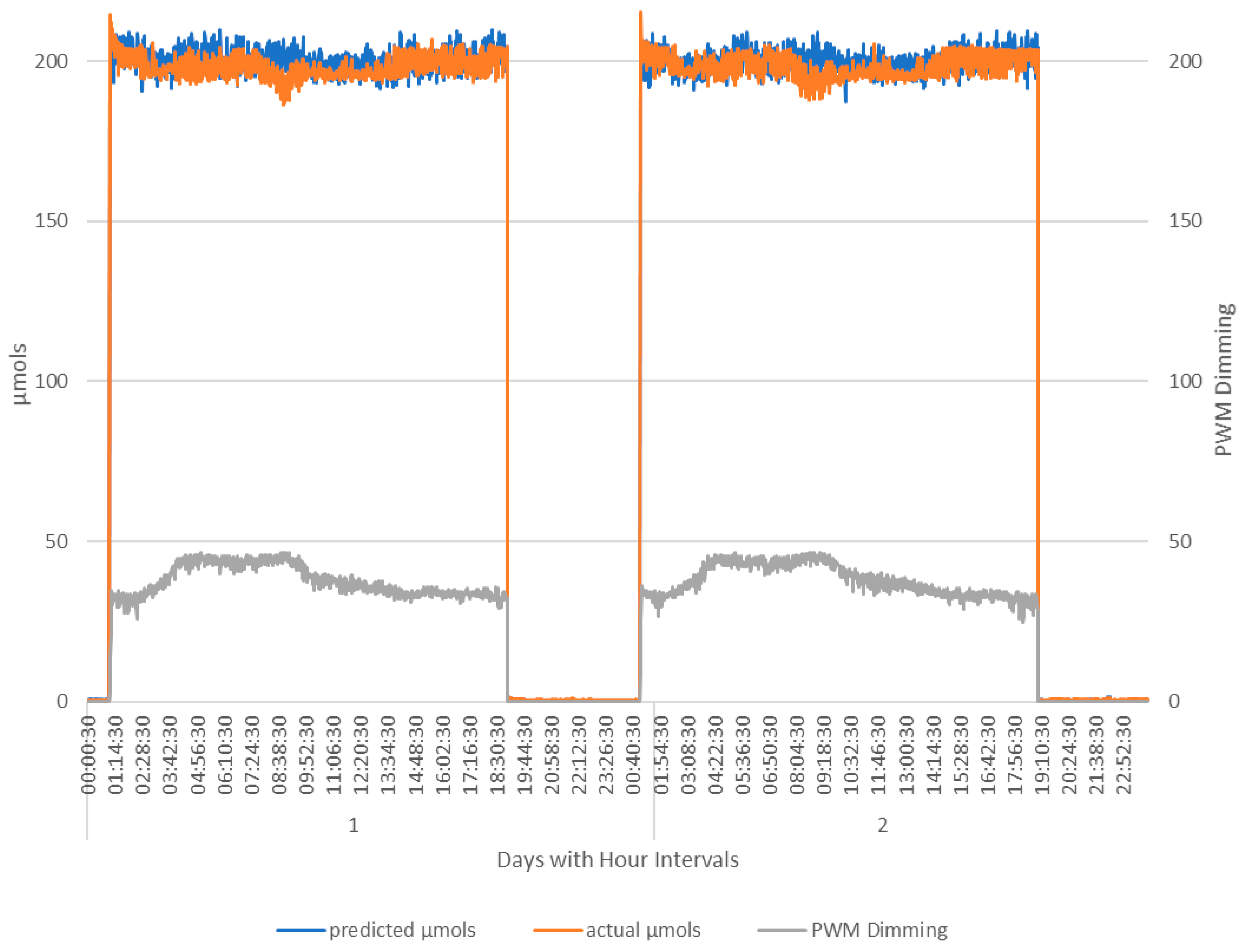
The AS7265x was used as the input for the PWM controller. Figure 13 tracks the sensor values with the PWM signal over two days. As the PAR light increases above 200 µmols, the PWM signal increases to dim lighting. When the PAR light comes back down to the threshold, the PWM signal also decreases maintaining a homeostasis. A Pearson’s Correlation was used to analyse this relationship and a strong positive correlation (r(60,480) = 0.963, p < 0.001) was found between the predicted µmols and the PWM dimming signal.
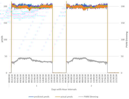
Figure 13.
Day one and two of phase two showing the system fully functional, with PWM Diming tracking closely with the PAR light readings. Note PWM increase during morning sunlight hours. PWM values are in the range 0–255. At 255, the lights are off. At 0, the lights are at full power.
The PWM’s strong significant correlation with the predicted µmols along with the evidence from phase one and minor differences between the AS7265x and Apogee SQ-520 combine to corroborate that a calibrated inexpensive IoT sensor can effectively replace the commercial-grade PAR light meter.
3.2. Plant Growth Results
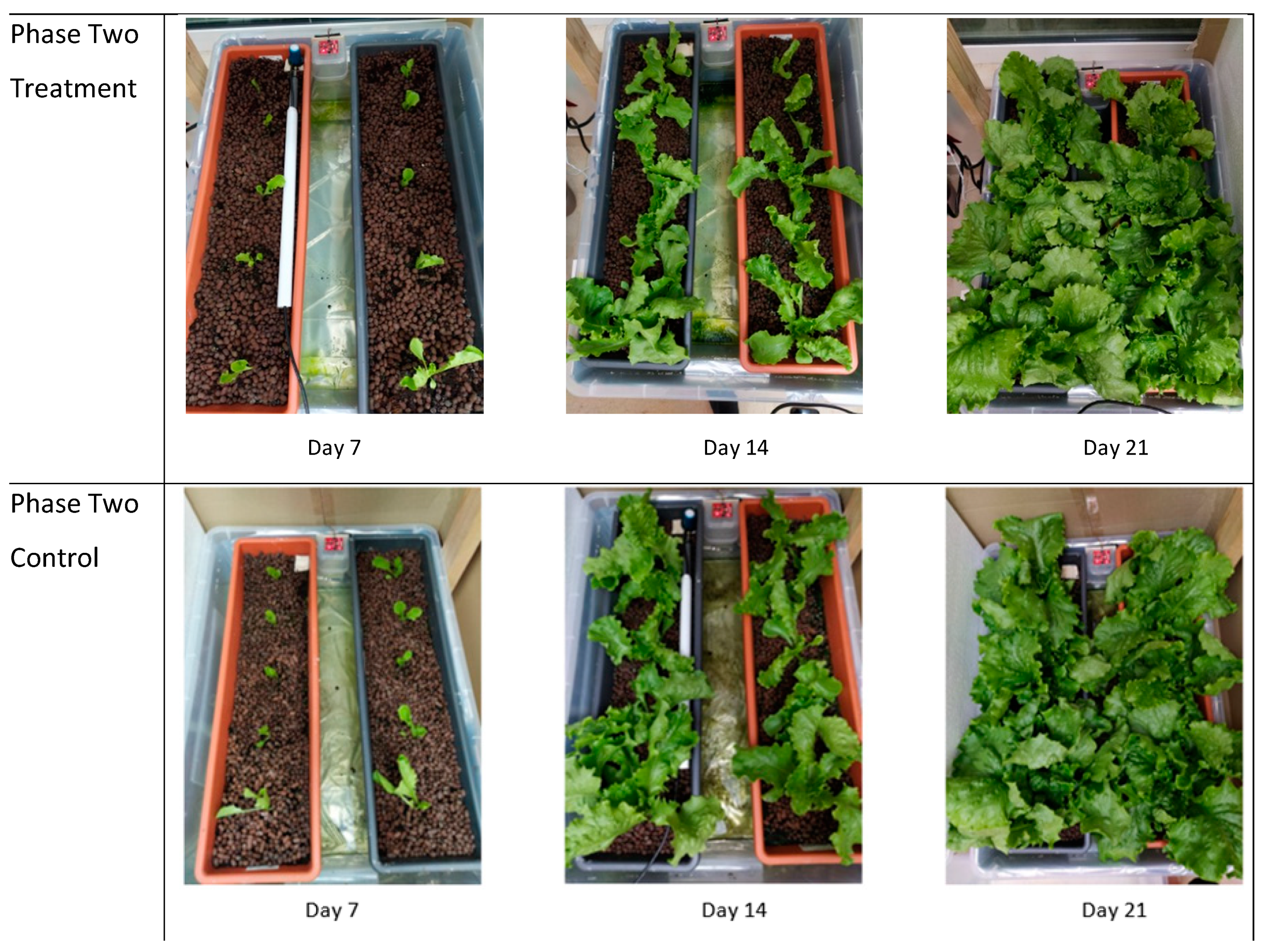
Plant growth performance for both phases, shown in Figure 14 and Figure 15, is reported in Table 4, which shows the total yield for fresh and dry weights along with the individual tray weights. The total yield for phase-one chambers differed greatly, while phase-two chambers were similar. A one-way ANOVA was used to determine if these differences were significant for both fresh and dry weights. The four lighting conditions resulted in a significant difference between the fresh weights (f(3, 36) = 63.68 p ≤ 0.001) and the dry weights (f(3, 36) = 87.54 p ≤ 0.001). A post hoc comparison was conducted using Tukey HSD, in Appendix C, to compare the means between chambers and yield measurement types. As expected, there is a large significant difference between fresh and dry yields in phase one, as noted in Table 5. The phase-two results were also as expected, with no significant difference between the fresh and dry weights. There was also no significant difference between the phase-one LED fresh weights and the phase-two treatment fresh weights. However, there was a small significant difference between the dry weights of the phase-one LED and the phase-two treatment. These results show the Adaptalight dimming system produces similar results as a standard light regime.
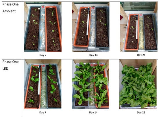
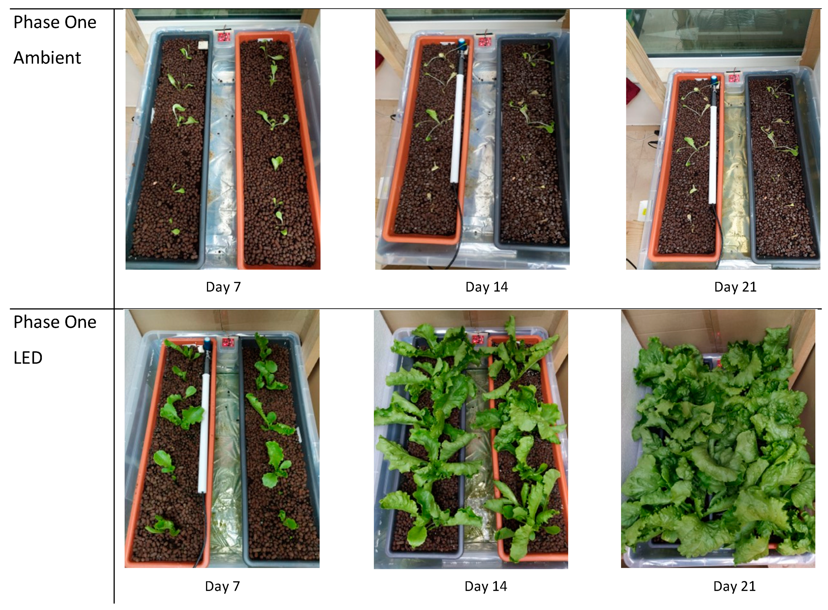
Figure 14.
Weekly pictures from the phase one, 21 day experiment.
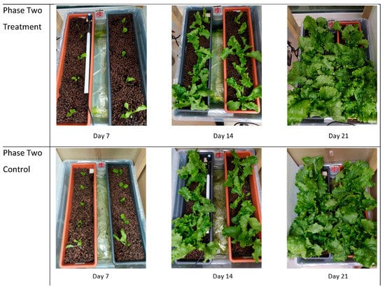
Figure 15.
Weekly pictures from the phase two, 21 day experiment.
Table 4.
Plant growth totals for phases one and two.
Table 5.
Means of the fresh and dry weight plant yields for phases one and two.
3.3. Power Consumption Results
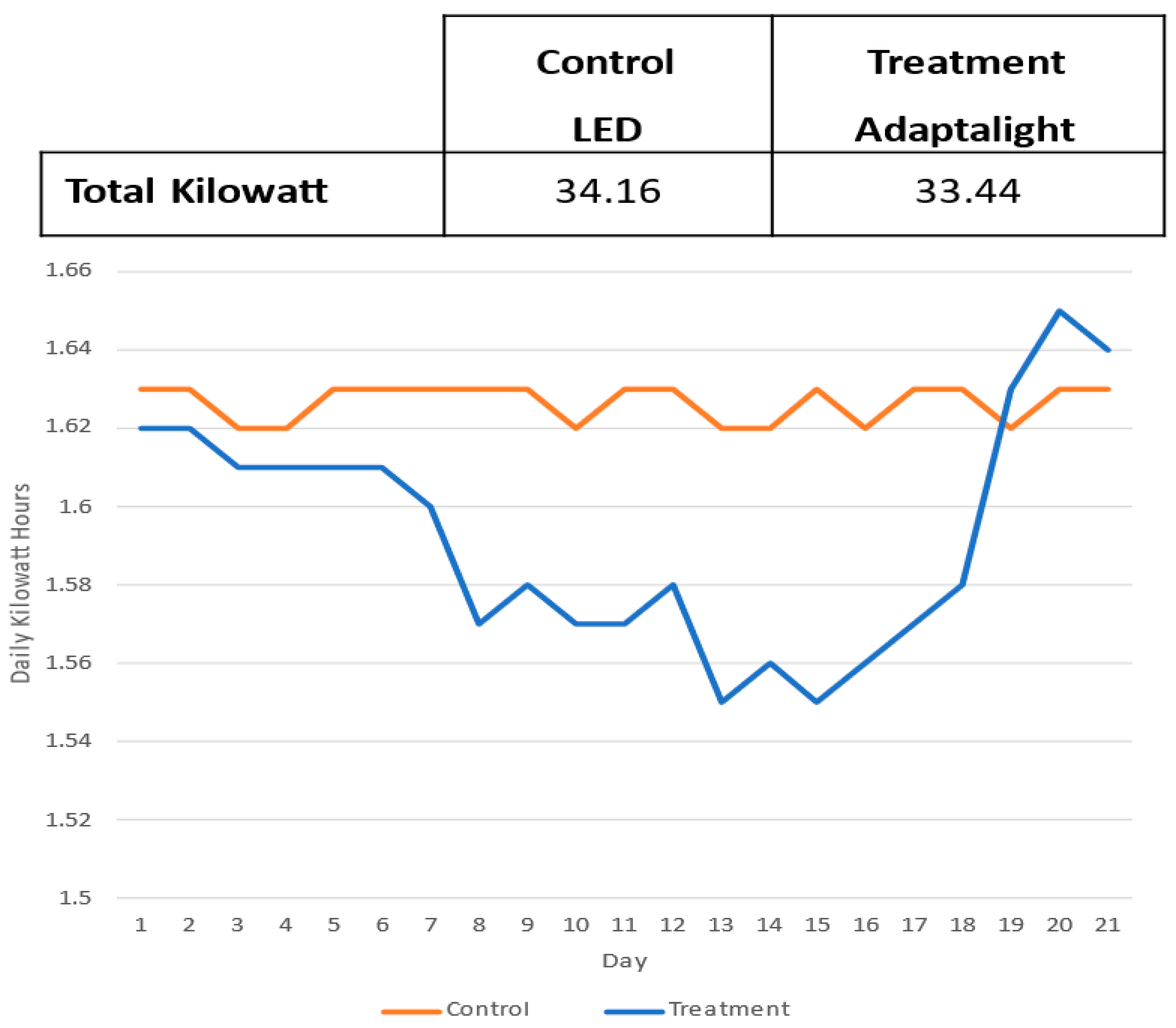
To determine if the Adaptalight dimming system was able to conserve power by modulating the lights, kilowatt hours were tracked and analysed in phase two between control and treatment chambers. Figure 16 shows the total kilowatts consumed each day of the experiment over the 21 day period. The LED luminaire in the control chamber was manually set to 200 µmols using an analogue potentiometer. It performed as expected, staying around 1.62 kWh and 1.63 kWh. The treatment was completely modulated from the system based on the amount of ambient light coming into the system. From day one to four, the Adaptalight system showed very slight differences of 0.01 kWh. However, as the experiment went on, the power conservation increased until the last three days when the ambient light was less, and the power increased to compensate. Over the 21 days, the total power consumption for the Adaptalight system was 0.72 kWh less than the control. In a scenario with more ambient light the power savings would have been greater.
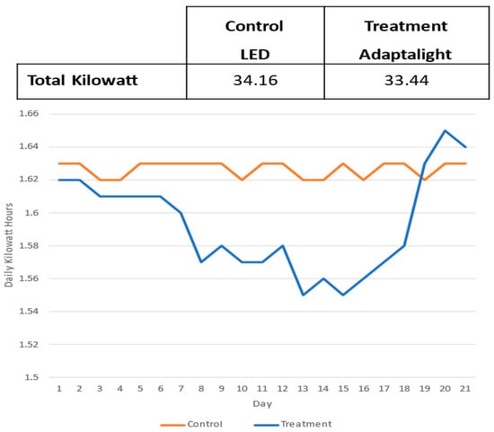
Figure 16.
Tracking the daily sum of kilowatt hour and the total kilowatt hours of control LED and the Adaptalight system treatment.
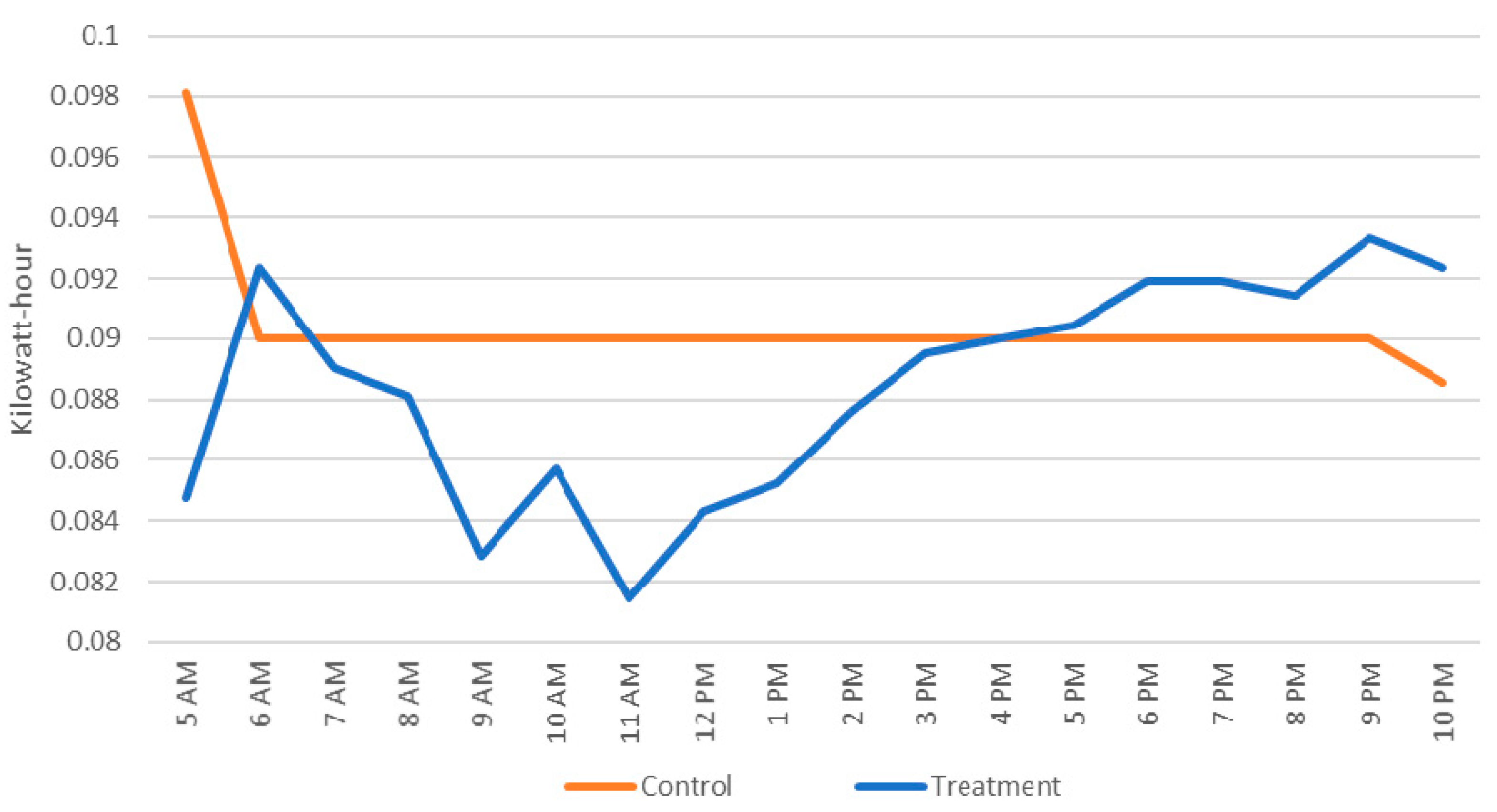
Figure 17 shows the hourly mean of each hour, across the 18 h photoperiod. As expected, the power consumption for the treatment drops in the afternoon and increases as the sun goes down. This is consistent with the PWM modulation shown in Figure 13. A two-sample t-test was used to determine if the Adaptalight system reduced the amount of power consumed compared to set standard lighting regime. The total mean of the treatment (M = 0.089, SD = 0.005) was significantly lower (t(754) = 6.108, p < 0.001) than the control (M = 0.090, SD = 0.002). While the difference is slight, it is significant, showing that the system does conserver power. To further eliminate other contributing factors that may be responsible for the reduction in power consumption, a two-way ANOVA was performed on the means of each hour by chamber. The results showed that there was significant interaction between the time of day and the chamber on the power consumption (f(17,720) = 20.76, p < 0.001). This further supported the notion that the time of day in the treatment chamber was responsible for the decreased power consumption.
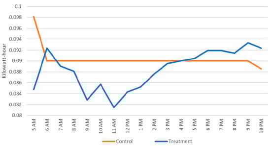
Figure 17.
The 21 day mean of each hour over the experiment.
4. Discussion
The results show that inexpensive IoT sensors work comparably to commercial sensors for measuring PAR in MISH systems. These results contribute to previous efforts, as shown in Table 1, to find PAR sensor alternatives. This enables citizen science and opens avenues of research into MISH systems, by increasing low-cost access to important metrics for building MISH lighting solutions. The results specifically favor the AS7265x sensor for measuring PAR light from various sources, supporting the findings of Leon-Salas et al. [28]. The limitations found of the TCS34725, in combination with the performance of models that included spectrums up to 910 nm, emphasize that an inexpensive sensor alternative must at minimum, cover the entire PAR spectrum range, and suggests that including far red and infra-red increases model accuracy.
A method for building calibration models was created. Unlike Lork et al. [30] and Mohagheghi and Moallem [34], the method of calibration does not require the knowledge of power consumption or the spectral composition of the light source. However, it does require a commercial sensor for initial calibration and recalibration when the sensor is repositioned. The results suggest the accuracy of the AS7265x to measure PAR is possibly attributed to the quality of the instrument that it is calibrated against. Leon-Salas et al. [28] used a single model to accurately measure ten different types of light sources, suggesting that a single calibration for the sensor to measure PAR light under all conditions is possible. The Adaptalight results show a pattern supporting this possibility. The phase-one LED model used for phase-two treatment chamber with only small adjustments successfully measured two different light sources simultaneously. While linear modelling calibration did not achieve the same accuracy as Leon-Salas et al.’s [28] vector quantization, one difference that may account for the accuracy gap was the lack of a light diffuser on the Adaptlight sensors.
The Adaptalight system used the SparkFun version of the AS7265x, it does not come with a dome light diffuser, like the AMS AS7265x evaluation kit used in Leon-Salas et al. [28]. This may be responsible for the exaggerated sensitivity observed while measuring sunlight, shown in Figure 11. At points, in Figure 16 and Figure 17, the power consumption surpasses that of the control lighting regime. This is likely due to the model values being anywhere from 8% to 18% greater than the actual values. This may have been reduced with the application of a diffuser. Additionally, calibrating the sensor with only LED light was the most effective way of harvesting daylight, any light beyond the baseline was easily identified and the system dimmed, even without the diffuser. However, irrespective of the diffuser, there is no question that this sensor can accurately measure PAR, possibly better than any other sensor at the time of this writing.
The Adaptalight system produced similar yields results to a standard lighting regime. It was noted that the yield from the LED chamber of the phase one is slightly higher than both chambers of phase two. While there were no significant differences in the fresh weights, the dry weights showed a small significant difference. This is most likely attributed to the size of the seedlings when transplanted into the system. Though all phases used 11-day-old seedlings grown from the same seed packet, seedlings for phase one were slightly larger as can be seen in the day seven images in Figure 14 and Figure 15. This would account for the small differences of dry weights.
The first-floor apartment had sun in a small area for a brief period of the day, during that time of the year. The goal was to measure this light and take it into account in the system. The sunlight had most affect near the window as seen in Figure 14 and Figure 15. The sensor was positioned nearest the window to harvest this light to save power. Placing additional sensors in the system to measure the back and side, as in Jiang et al. [33] and Mohagheghi and Moallem [34] would not contribute to this and was beyond the scope of this study. Even under these minimal conditions, the system harvested the small bit of daylight coming into the system. This is promising for the future of daylight harvesting in MISH-O systems. Future work may re-run these tests in different locations to further document the power savings capabilities.
It was beyond the scope of this study to address the nutrient aspect of the plant growth. To control for this, both chambers were given nutrient solutions from the same reservoir. The nutrient reservoir was large enough that there was no need to adjust the pH or EC through the experiments. Another aspect beyond the scope of this study was to examine the affects of the apartment window glazing on the PAR light coming into the system, as noted in Dangol et al. [49]. Finally, temperatures during sunlight hours were also considered beyond the scope of this study. Because it is an open system and was conducted in the living room of an apartment where the thermostat regulated the temperature to 23 °C, all phases of the experiment were maintained at the same temperature.
5. Conclusions
This study proposed the Adaptalight MISH-O system, using inexpensive IoT sensors for measuring PAR accurately and harvesting ambient light to save energy. The system was constructed using entirely locally sourced components and was successfully demonstrated in a home setting in Dubai, UAE. This study shows that the low-cost solutions can sufficiently measure PAR values from artificial and natural light simultaneously. Using a $50 commodity IoT sensor to perform in place of a $500 commercial PAR sensor. The Adaptalight system modified LED light according to PAR values from the calibrated AS7265x, to maintain threshold settings. There was no significant difference between the plant yields when compared to the controls. The system design and inexpensive PAR sensor alternative enables ordinary citizens to build energy efficient MISH-O systems to grow food at home. The findings also support the AS7265x sensor as the best suited sensor to economically measure PAR.
Further research is required to improve the calibration methodology to establish a one-time calibration for the AS7265x. Additionally, more research is needed to determine if there is a need for a PAR level of precision in MISH-O settings.
Author Contributions
Conceptualization, J.D.S., D.M., D.D. and D.T.; methodology, J.D.S., D.M., D.D. and D.T.; investigation, J.D.S.; formal analysis, J.D.S.; writing—original draft preparation, J.D.S.; writing—review and editing, J.D.S., D.M. and D.T. All authors have read and agreed to the published version of the manuscript.
Funding
This research received no external funding.
Institutional Review Board Statement
Not applicable.
Informed Consent Statement
Not applicable.
Conflicts of Interest
The authors declare no conflict of interest.
Appendix A
Table A1.
Model coefficients deployed in phase one that were produced with a data set collected over 5 days. For this phase, the sun side used a separate data set from the LED side.
Table A1.
Model coefficients deployed in phase one that were produced with a data set collected over 5 days. For this phase, the sun side used a separate data set from the LED side.
| Phase-One Deployed Linear Models | ||
|---|---|---|
| Ambient Light | LED Light | |
| Goodness of fit | R2 = 88.7 MSE = 56.945 | R2 = 99.8 MSE = 22.78 |
| Intercept | 0.579 | 0.417 |
| 410 nm | −1.87 | 0.833 |
| 435 nm | 1.925 | −0.015 |
| 460 nm | −0.918 | 0.008 |
| 485 nm | 2.053 | −0.037 |
| 510 nm | −1.32 | 0.064 |
| 535 nm | −0.378 | −0.070 |
| 560 nm | 0.528 | 0.033 |
| 585 nm | −1.984 | −0.036 |
| 610 nm | 0.319 | 0.009 |
| 645 nm | 0.814 | 0.008 |
| 680 nm | 0.143 | 0.069 |
| 705 nm | 0.987 | −0.235 |
| 730 nm | −0.943 | 0.135 |
| 760 nm | 3.159 | −0.060 |
| 810 nm | −3.653 | −0.657 |
| 860 nm | 0.105 | 0.721 |
| 900 nm | 0.524 | −0.446 |
| 940 nm | 2.234 | −0.244 |
Appendix B
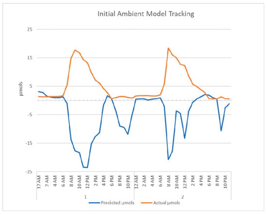
Figure A1.
The first two days of the deployed ambient model, the inverse relationship between the actual results and the predicted results are shown here.
Figure A1.
The first two days of the deployed ambient model, the inverse relationship between the actual results and the predicted results are shown here.
Appendix C
Table A2.
Phases One and Two Fresh Weight ANOVA Tukey Post hoc HSD.
Table A2.
Phases One and Two Fresh Weight ANOVA Tukey Post hoc HSD.
| (I) Chamber | (J) Chamber | Mean Difference (I–J) | Std. Error | Sig. | Lower Bound | Upper Bound |
|---|---|---|---|---|---|---|
| P1-Ambient-Control | P1-LED Treatment | −91.40 | 7.96 | 0.00 | −112.83 | −69.98 |
| P2-Ambient + LED-Treatment | −89.24 | 7.96 | 0.00 | −110.66 | −67.81 | |
| P2-LED-Control | −88.62 | 7.96 | 0.00 | −110.04 | −67.19 | |
| P1-LED Treatment | P1-Ambient-Control | 91.40 | 7.96 | 0.00 | 69.98 | 112.83 |
| P2-Ambient + LED-Treatment | 2.17 | 7.96 | 0.99 | −19.26 | 23.59 | |
| P2-LED-Control | 2.79 | 7.96 | 0.99 | −18.64 | 24.21 | |
| P2-Ambient + LED-Treatment | P1-Ambient-Control | 89.24 | 7.96 | 0.00 | 67.81 | 110.66 |
| P1-LED Treatment | −2.17 | 7.96 | 0.99 | −23.59 | 19.26 | |
| P2-LED-Control | 0.62 | 7.96 | 1.00 | −20.81 | 22.05 | |
| P2-LED-Control | P1-Ambient-Control | 88.62 | 7.96 | 0.00 | 67.19 | 110.04 |
| P1-LED Treatment | −2.79 | 7.96 | 0.99 | −24.21 | 18.64 | |
| P2-Ambient + LED-Treatment | −0.62 | 7.96 | 1.00 | −22.05 | 20.81 | |
| Phases One and Two Dry Weight ANOVA Tukey Post hoc HSD | ||||||
| (I) Chamber | (J) Chamber | Mean Difference (I–J) | Std. Error | Sig. | Lower Bound | Upper Bound |
| P1-Ambient-Control | P1-LED Treatment | −4.47 | 0.28 | 0.000 | −5.23 | −3.70 |
| P2-Ambient + LED-Treatment | −3.04 | 0.28 | 0.000 | −3.80 | −2.27 | |
| P2-LED-Control | −3.01 | 0.28 | 0.000 | −3.77 | −2.24 | |
| P1-LED Treatment | P1-Ambient-Control | 4.47 | 0.28 | 0.000 | 3.70 | 5.23 |
| P2-Ambient + LED-Treatment | 1.43 | 0.28 | 0.000 | 0.66 | 2.20 | |
| P2-LED-Control | 1.46 | 0.28 | 0.000 | 0.69 | 2.23 | |
| P2-Ambient + LED-Treatment | P1-Ambient-Control | 3.04 | 0.28 | 0.000 | 2.27 | 3.80 |
| P1-LED Treatment | −1.43 | 0.28 | 0.000 | −2.20 | −0.66 | |
| P2-LED-Control | 0.03 | 0.28 | 1.000 | −0.74 | 0.80 | |
| P2-LED-Control | P1-Ambient-Control | 3.01 | 0.28 | 0.000 | 2.24 | 3.77 |
| P1-LED Treatment | −1.46 | 0.28 | 0.000 | −2.23 | −0.69 | |
| P2-Ambient + LED-Treatment | −0.03 | 0.28 | 1.000 | −0.80 | 0.74 | |
Appendix D
Table A3.
Model 4 coefficients for AS7265x produced with the 5 day combined data set. This was the model used in the full system deployment.
Table A3.
Model 4 coefficients for AS7265x produced with the 5 day combined data set. This was the model used in the full system deployment.
| AS7265x Model 4 Linear Model Coefficients | |
|---|---|
| Intercept | −1.101 |
| 410 nm | 0.647 |
| 435 nm | −0.044 |
| 460 nm | −0.146 |
| 485 nm | 0.074 |
| 510 nm | 0.384 |
| 535 nm | −0.385 |
| 560 nm | 0.472 |
| 585 nm | −0.282 |
| 610 nm | 0.067 |
| 645 nm | −0.182 |
| 680 nm | 0.003 |
| 705 nm | 0.602 |
| 730 nm | −0.093 |
| 760 nm | −0.737 |
| 810 nm | 0.542 |
| 860 nm | 0.770 |
| 900 nm | 0.091 |
| 940 nm | −2.785 |
References
- United Nations Global Issues Overview. Available online: https://www.un.org/en/sections/issues-depth/global-issues-overview/index.html (accessed on 16 August 2020).
- Knorr, D.; Khoo, C.S.H.; Augustin, M.A. Food for an Urban Planet: Challenges and Research Opportunities. Front. Nutr. 2018, 4, 73. [Google Scholar] [CrossRef]
- Food and Agriculture Organization of the United Nations. The Future of Food and Agriculture: Trends and Challenges; FAO: Rome, Italy, 2017; ISBN 9789251095515. [Google Scholar]
- Dongyu, Q. Senior Officials Sound Alarm over Food Insecurity, Warning of Potentially ‘Biblical’ Famine, in Briefings to Security Council. Available online: https://www.un.org/press/en/2020/sc14164.doc.htm (accessed on 20 January 2022).
- Katz, H. Crisis gardening: Addressing barriers to home gardening during the COVID-19 pandemic. Austrailan Food Netw. Melb. Aust. 2020, 1–47. Available online: https://sustain.org.au/media/blog/Crisis-Gardening-Addressing-Barriers-to-Home-Gardening-during-the-COVID-19-Pandemic.-.pdf (accessed on 20 January 2022).
- Lal, R. Home gardening and urban agriculture for advancing food and nutritional security in response to the COVID-19 pandemic. Food Secur. 2020, 12, 871–876. [Google Scholar] [CrossRef]
- Nicola, S.; Ferrante, A.; Cocetta, G.; Bulgari, R.; Nicoletto, C.; Sambo, P.; Ertani, A. Food Supply and Urban Gardening in the Time of COVID-19. Bull. UASVM Hortic. 2020, 77, 141. [Google Scholar] [CrossRef]
- Mullins, L.; Charlebois, S.; Finch, E.; Music, J. Home food gardening in Canada in response to the COVID-19 pandemic. Sustainability 2021, 13, 3056. [Google Scholar] [CrossRef]
- Pulighe, G.; Lupia, F. Food First: COVID-19 Outbreak and Cities Lockdown a Booster for a Wider Vision on Urban Agriculture. Sustainability 2020, 12, 5012. [Google Scholar] [CrossRef]
- Stevens, J.D.; Shaikh, T. MicroCEA: Developing a Personal Urban Smart Farming Device. In Proceedings of the 2018 2nd International Conference on Smart Grid and Smart Cities (ICSGSC), Kuala Lumpur, Malaysia, 12–14 August 2018. [Google Scholar]
- Harper, C.; Siller, M. OpenAG: A Globally Distributed Network of Food Computing. IEEE Pervasive Comput. 2015, 14, 24–27. [Google Scholar] [CrossRef]
- AeroGrow Interanational Inc. Bounty Basic. Available online: https://www.aerogarden.com/aerogarden-bounty-basic.html (accessed on 26 July 2020).
- Bhuiyan, R.; van Iersel, M.W. Only Extreme Fluctuations in Light Levels Reduce Lettuce Growth Under Sole Source Lighting. Front. Plant Sci. 2021, 12, 24. [Google Scholar] [CrossRef]
- Arcel, M.M.; Lin, X.; Huang, J.; Wu, J.; Zheng, S. The application of LED illumination and intelligent control in plant factory, a new direction for modern agriculture: A Review. J. Phys. Conf. Ser. 2021, 1732, 012178. [Google Scholar] [CrossRef]
- Silvertown, J. A new dawn for citizen science Jonathan. Trends Ecol. Evol. 2009, 24, 467–471. [Google Scholar] [CrossRef]
- Ferreira, A.J.D.; Guilherme, R.I.M.M.; Ferreira, C.S.S.; de Oliveira, M.d.F.M.L. Urban agriculture, a tool towards more resilient urban communities? Curr. Opin. Environ. Sci. Health 2018, 5, 93–97. [Google Scholar] [CrossRef]
- Edmondson, J.L.; Blevins, R.S.; Cunningham, H.; Dobson, M.C.; Leake, J.R.; Grafius, D.R. Grow your own food security? Integrating science and citizen science to estimate the contribution of own growing to UK food production. Plants People Planet 2019, 1, 93–97. [Google Scholar] [CrossRef]
- Pollard, G.; Roetman, P.; Ward, J. The case for citizen science in urban agriculture research. Future Food J. Food Agric. Soc. 2017, 5, 9–20. [Google Scholar]
- Ryan, S.F.; Adamson, N.L.; Aktipis, A.; Andersen, L.K.; Austin, R.; Barnes, L.; Beasley, M.R.; Bedell, K.D.; Briggs, S.; Chapman, B.; et al. The role of citizen science in addressing grand challenges in food and agriculture research. Proc. R. Soc. B Biol. Sci. 2018, 285, 20181977. [Google Scholar] [CrossRef]
- Lopez-Novoa, U.; Morgan, J.; Jones, K.; Rana, O.; Edwards, T.; Grigoletto, F. Enabling citizen science in rural environments with IoT and mobile technologies. CEUR Workshop Proc. 2019, 2530, 50–56. [Google Scholar]
- Woodward, F.I. Instruments for the Measurement of Photosynthetically Active Radiation and Red, Far-Red and Blue Light. J. Appl. Ecol. 1983, 20, 103. [Google Scholar] [CrossRef]
- Fielder, P.; Comeau, P. Construction and Testing of an Inexpensive PAR Sensor: Peter Fielder and Phil Comeau; Crown Publications: Victoria, BC, Canada, 2000; pp. 1–32.
- Barnard, H.R.; Findley, M.C.; Csavina, J. PARduino: A simple and inexpensive device for logging photosynthetically active radiation. Tree Physiol. 2014, 34, 640–645. [Google Scholar] [CrossRef]
- Kuhlgert, S.; Austic, G.; Zegarac, R.; Osei-Bonsu, I.; Hoh, D.; Chilvers, M.I.; Roth, M.G.; Bi, K.; TerAvest, D.; Weebadde, P.; et al. MultispeQ Beta: A tool for large-scale plant phenotyping connected to the open PhotosynQ network. R. Soc. Open Sci. 2016, 3, 160592. [Google Scholar] [CrossRef] [Green Version]
- Caya, M.V.C.; Alcantara, J.T.; Carlos, J.S.; Cereno, S.S.B. Photosynthetically Active Radiation (PAR) Sensor Using an Array of Light Sensors with the Integration of Data Logging for Agricultural Application. In Proceedings of the 2018 3rd International Conference on Computer and Communication Systems (ICCCS), Nagoya, Japan, 27–30 April 2018; pp. 431–435. [Google Scholar] [CrossRef]
- Kutschera, A.; Lamb, J.J. Light Meter for Measuring Photosynthetically Active Radiation. Am. J. Plant Sci. 2018, 9, 2420–2428. [Google Scholar] [CrossRef] [Green Version]
- Adhiwibawa, M.A.; Kurniawan, J.M. Simple Photometer Development For Educational Purposes in Natural Pigment Analysis. Indones. J. Nat. Pigment. 2020, 2, 17. [Google Scholar] [CrossRef]
- Leon-Salas, W.D.; Rajendran, J.; Vizcardo, M.A.; Postigo-Malaga, M. Measuring Photosynthetically Active Radiation with a Multi-Channel Integrated Spectral Sensor. In Proceedings of the 2021 IEEE International Symposium on Circuits and Systems (ISCAS), Daegu, Korea, 22–28 May 2021; pp. 1–5. [Google Scholar] [CrossRef]
- Nedbal, J.; Gao, L.; Suhling, K. Bottom-illuminated orbital shaker for microalgae cultivation. HardwareX 2020, 8, e00143. [Google Scholar] [CrossRef] [PubMed]
- Lork, C.; Cubillas, M.; Kiat Ng, B.K.; Yuen, C.; Tan, M. Minimizing Electricity Cost through Smart Lighting Control for Indoor Plant Factories. In Proceedings of the IECON 2020 the 46th Annual Conference of the IEEE Industrial Electronics Society, Singapore, 18–21 October 2020; pp. 297–302. [Google Scholar] [CrossRef]
- Johnson, A.J.; Meyerson, E.; de la Parra, J.; Savas, T.; Miikkulainen, R.; Harper, C. Flavor-Cyber-Agriculture: Optimization of plant metabolites in an open-source control environment through surrogate modeling. PLoS ONE 2019, 14, e0213918. [Google Scholar] [CrossRef] [PubMed] [Green Version]
- Thimijan, R.; Heins, R. Photometric, radiometric, and quantum light units of measure: A review of procedures for interconversion. HortScience 1983, 18, 818–822. [Google Scholar]
- Jiang, J.; Moallem, M.; Zheng, Y. An intelligent iot-enabled lighting system for energy-efficient crop production. J. Daylighting 2021, 8, 86–99. [Google Scholar] [CrossRef]
- Mohagheghi, A.; Moallem, M. Intelligent Spectrum Controlled Supplemental Lighting for Daylight Harvesting. IEEE Trans. Ind. Inform. 2021, 17, 3263–3272. [Google Scholar] [CrossRef]
- Chang, C.-W.; David, A.L.; Maurice, J.M.; Charles, R.H. Near-Infrared Reflectance Spectroscopy–Principal Components RegressionAnalyses of Soil Properties. Soil Sci. Soc. Am. J. 2001, 65, 480–490. [Google Scholar] [CrossRef] [Green Version]
- Attarchi, S.; Moallem, M. Set-point control of LED luminaires for daylight harvesting. In Proceedings of the 2017 5th International Conference on Control, Instrumentation, and Automation (ICCIA), Shiraz, Iran, 21–23 November 2017; pp. 244–248. [Google Scholar] [CrossRef]
- González-Amarillo, C.A.; Cárdenas-García, C.L.; Caicedo-Muñoz, J.A.; Mendoza-Moreno, M.A. Smart Lumini: A Smart Lighting System for Academic Environments Using IOT-Based Open-Source Hardware. Rev. Fac. Ing. 2020, 29, e11060. [Google Scholar] [CrossRef]
- Ryer, A. Light Measurement Handbook, 2nd ed.; International Light: Newburyport, MA, USA, 1997; ISBN 0-9658356-9-3. [Google Scholar]
- Peffers, K.; Tuunanen, T.; Rothenberger, M.A.; Chatterjee, S. A design science research methodology for information systems research. J. Manag. Inf. Syst. 2007, 24, 45–77. [Google Scholar] [CrossRef]
- Adamson, H.P.; Kruglak, I.T. Adaptive Photosynthetically Active Radiation (PAR) Sensor with Daylight Integral (DLI) Control System Incorporating Lumen Maintenance. U.S. Patent 16/384,573, 24 October 2019. [Google Scholar]
- Wojciechowska, R.; Dugosz-Grochowska, O.; Koton, A.; Zupnik, M. Effects of LED supplemental lighting on yield and some quality parameters of lamb’s lettuce grown in two winter cycles. Sci. Hortic. 2015, 187, 80–86. [Google Scholar] [CrossRef]
- Hang, T.; Lu, N.; Takagaki, M.; Mao, H. Leaf area model based on thermal effectiveness and photosynthetically active radiation in lettuce grown in mini-plant factories under different light cycles. Sci. Hortic. 2019, 252, 113–120. [Google Scholar] [CrossRef]
- Loconsole, D.; Cocetta, G.; Santoro, P.; Ferrante, A. Optimization of LED lighting and quality evaluation of Romaine lettuce grown in an innovative indoor cultivation system. Sustainability 2019, 11, 841. [Google Scholar] [CrossRef] [Green Version]
- Palmer, S.; van Iersel, M.W. Increasing growth of lettuce and mizuna under sole-source LED lighting using longer photoperiods with the same daily light integral. Agronomy 2020, 10, 1659. [Google Scholar] [CrossRef]
- Brechner, M.; Both, A.; Cornell CEA Staff. Hydroponic Lettuce Handbook; Cornell University: Ithaca, NY, USA, 1996. [Google Scholar]
- Kozai, T.; Niu, G.; Takagaki, M. Plant Factory: An Indoor Vertical Farming System for Efficient Quality Food Production, 2nd ed.; Academic Press: Cambridge, MA, USA, 2019; ISBN 9780128017753. [Google Scholar]
- Zhang, X.; He, D.; Niu, G.; Yan, Z.; Song, J. Effects of environment lighting on the growth, photosynthesis, and quality of hydroponic lettuce in a plant factory. Int. J. Agric. Biol. Eng. 2018, 11, 33–40. [Google Scholar] [CrossRef]
- Paz, M.; Fisher, P.R.; Gómez, C. Minimum Light Requirements for Indoor Gardening of Lettuce. Urban Agric. Reg. Food Syst. 2019, 4, 1–10. [Google Scholar] [CrossRef] [Green Version]
- Dangol, R.; Kruisselbrink, T.; Rosemann, A. Effect of window glazing on colour quality of transmitted daylight. J. Daylighting 2017, 4, 37–47. [Google Scholar] [CrossRef] [Green Version]


Publisher’s Note: MDPI stays neutral with regard to jurisdictional claims in published maps and institutional affiliations. |
© 2022 by the authors. Licensee MDPI, Basel, Switzerland. This article is an open access article distributed under the terms and conditions of the Creative Commons Attribution (CC BY) license (https://creativecommons.org/licenses/by/4.0/).