The U.S. Sweet Potato Market: Price Response and Impact of Supply Shocks

Abstract

Sweet potatoes have become increasingly popular among consumers due to their health benefits, and, as a result, sweet potato production has been growing rapidly over the last decade in the United States. However, the industry is facing major challenges, including the risk of disease outbreaks and adverse weather events, which could potentially have a significant impact on the market. However, the economic literature on the sweet potato commodity is limited. This study models the U.S. sweet potato market price response to supply changes and derives elasticity estimates. This information is essential for understanding the sweet potato market and for simulating the impacts of potential supply shocks, given the challenges that the industry is facing. We found that prices are highly sensitive to supply. North Carolina, the largest sweet potato producer in the country, dominates the domestic market and exerts significantly larger influences on market prices than other producing states.

1. Introduction

The United States is one of the major sweet potato suppliers in the world, and produced 1,624,277 tons of sweet potatoes in 2019 [1]. According to the export statistics published by the Food and Agriculture Organization of the United Nations [1], the United States is the country with the largest quantity of sweet potato exports over the past decade. The total quantity of U.S. sweet potato exports reached 261,452 tons in 2019, valued at $188.3 million. U.S. exports account for about 27% of the total sweet potato exports in the world. North Carolina is the top ranked state of sweet potato production in the U.S., accounting for 61.1% of the total U.S. production in 2019 [2].

In recent years, sweet potato production in the U.S. has encountered several challenges, including trade disputes, volatile weather, and pest and disease issues, which could significantly impact the growth of the industry. For instance, a new nematode pest called the guava root knot nematode (Meloidogyne enterolobii) has been found across the southeastern states in recent years, which could cause severe damage to the production of sweet potatoes and threaten the sustainability of the local farming sector. These challenges have received attention from both growers and policymakers. Yield loss due to production challenges will result in supply shocks in the market, which will drive market price fluctuations. As the total quantity of sweet potatoes produced decreases, the market price would increase, which could alleviate the economic impact of yield declines. On the other hand, a spike in production (market supply) could cause prices to drop, thus dampening the benefits of increased production or yield. As a result, to accurately assess the economic impacts of changes in the sweet potatoes supply, it is important to estimate market price responses, which is essential information for assessing the economic impacts of shocks or changes in the industry.

For centuries, the sweet potato has been a fundamental part of the human diet and is still an important food for underdeveloped countries today [3,4]. Interestingly, sweet potatoes have only become a highly consumed product recently in developed countries [4,5], even though the total production has shown a decline over the past few decades [6]. Although China, Bangladesh, and several countries on the African continent are also among the world’s major producers [4,7], sweet potatoes have long been cultivated throughout the American continent since before colonial times [4]; and today, sweet potatoes are an increasingly popular vegetable in developed economies due to their health benefits [7].

China has had a prominent role in sweet potato production since the 1960s, where the sweet potato is a substitute for potatoes and is less sensitive to changes in consumer income [8]. In the U.S., sweet potato consumption has been increasing, and it is a crop consumed throughout the year [5]. Despite the popularity that this crop has gained in recent years, we know very little about the behavior of sweet potato consumers in the U.S.

In the U.S., the high level of geographical concentration for the production of sweet potatoes means that diseases and adverse weather events could have serious impacts on production, and thus threaten supplies [4]. The goal of this study is to quantify the effect of quantity changes on the market price of sweet potatoes in the U.S. market. This is the first research that examines the relationship between the supply and market prices of sweet potatoes in the U.S. market. Using sweet potato production information in the United States, the relationship between market prices and supply changes across different regions is investigated. The study shows how the yield changes in one state would affect the market prices of sweet potatoes in its own state, as well as in other states.

In this research, we use an inverse demand system to answer the question: how would sweet potato consumers react in terms of the prices they would pay if there were a supply shock? Such shocks could be the result of disease outbreaks or weather events. As sweet potatoes become one of the important crops in the U.S. farming sector, particularly in major producing states such as North Carolina, California, Mississippi, and Louisiana, the analysis of the linkage between supply and price is important and of high demand among growers and policymakers. As climate change accelerates, challenges to sweet potato cultivation, such as volatile weather and high disease pressure, could pose increasing threats to the industry. This study could provide growers and policymakers with useful information and insights into the potential economic ramifications of these challenges and inform policymaking.

The Sweet Potato Market in the U.S.

Sweet potato is an important food crop worldwide, along with other crops such as rice, corn, wheat, and potatoes [9]. Sweet potatoes are hardy crops that are rich in carbohydrates, vitamins, and minerals; they are also high in edible energy compared to other food crops such as rice and wheat [9]. As a result, sweet potatoes are widely grown all over the world, and due to the large demand in the international market, the export of sweet potatoes has continued to grow over the years [1]. Moreover, because of characteristics such as versatility, adaptability to various climates, and importance for food security and farm income, sweet potatoes have received increasing attention in research [10]. There are about 117 countries growing sweet potatoes, and the total production was about 91.95 million tons [1]. China is the largest sweet potato producing country, with a total of 53.01 million tons in 2018 [1], and the United State is the largest sweet potato exporting country, with a total of 300,981 tons exported in 2018 [1]. The main destinations of U.S. exported sweet potatoes were the European Union (40%), UK (30%), and Canada (24%).

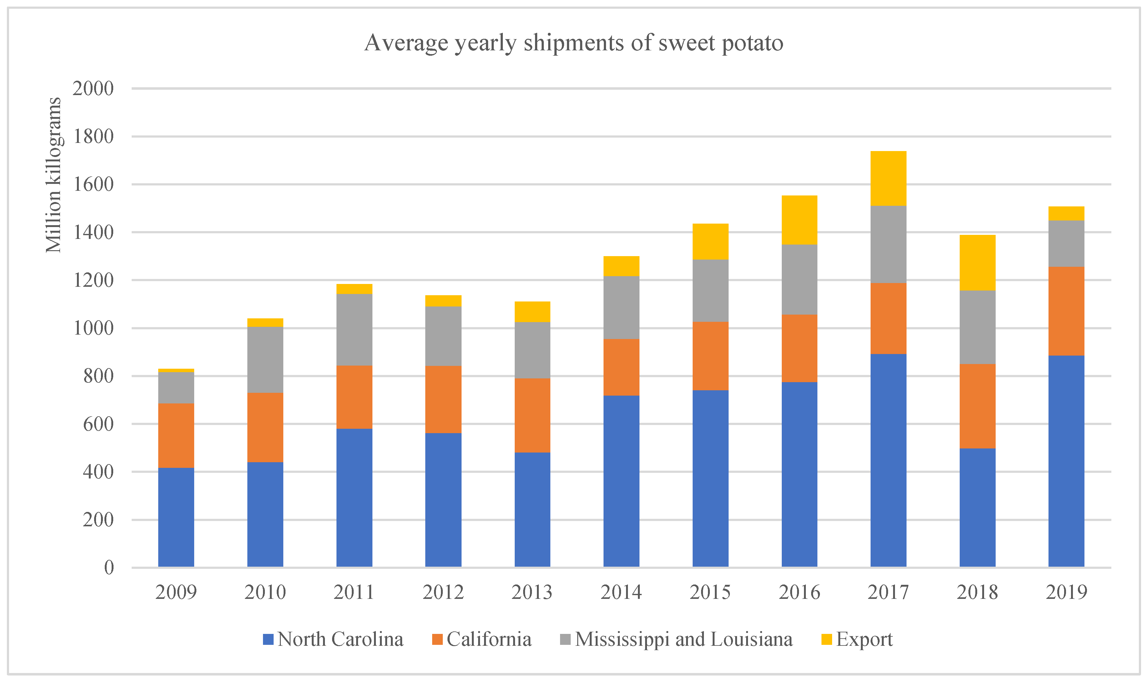
Figure 1 shows the statistics of U.S. sweet potato production and exports over the period 2009–2019. As can be seen, the total shipment of sweet potatoes in the U.S. has been increasing over the years, from about 800 million kg in 2009 to over 1700 million kg in 2017. The total amount of sweet potato production decreased notably to about 1400 million kg in 2018 because North Carolina was hit by the destructive Hurricane Michael, which severely affected production. The total production of sweet potatoes dropped by more than 40% in North Carolina [11], marking the lowest level of production in 5 years. The results in Figure 1 show that the production of sweet potatoes is quite vulnerable to severe weather damage. Similar weather events may occur more frequently in the future as climate change accelerates.

The results in Figure 1 also show that the largest supplier of sweet potatoes in the U.S. is North Carolina, which contributed to more than half of the sweet potato production over the years. Other states such as California, Mississippi, and Louisiana take a relatively smaller share of the total production, and the quantity of these states are similar and have remained stable over the years. The export of sweet potatoes, as mentioned before, has made the U.S. a major competitor and supplier in the global market. However, exports were clearly affected in 2019 due to the fact that North Carolina was hit by hurricanes and experienced a significant reduction in sweet potato production.

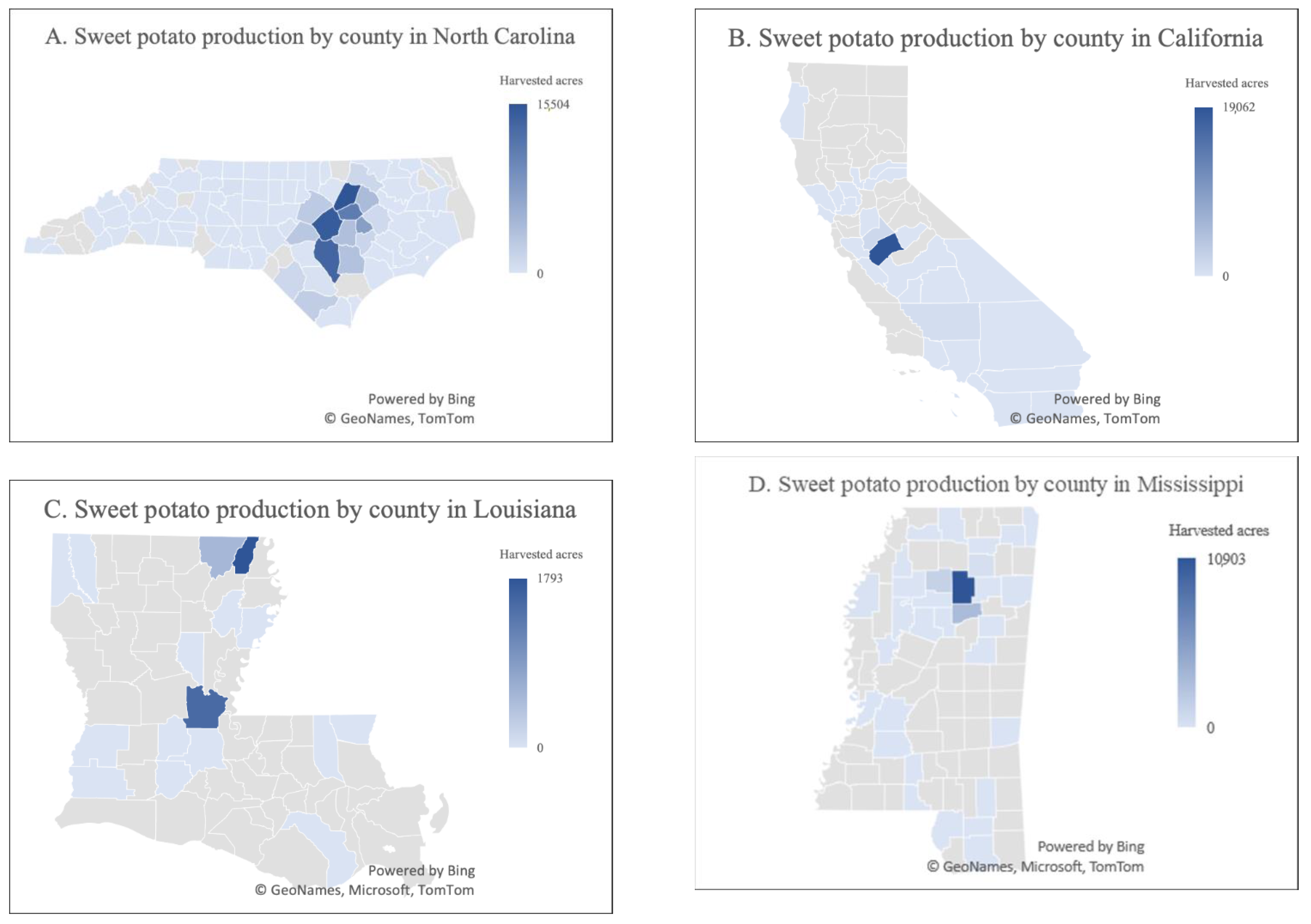
Figure 2 shows the distribution of sweet potato production in four major states. As can be seen, the growing of sweet potato is generally concentrated within one or a few counties in these states. The counties in North Carolina with the highest levels of sweet potato production are Sampson county, Johnston county, and Nash county. Meanwhile, the counties that are adjacent to these three counties are also sweet potato production counties, but with a smaller production scale. California and Mississippi share the same spatial patterns; only one county stands out as the major supplier for the whole state, while other counties produce at a significantly smaller scale. The production of sweet potatoes in Louisiana is concentrated in two counties that are distant from each other.

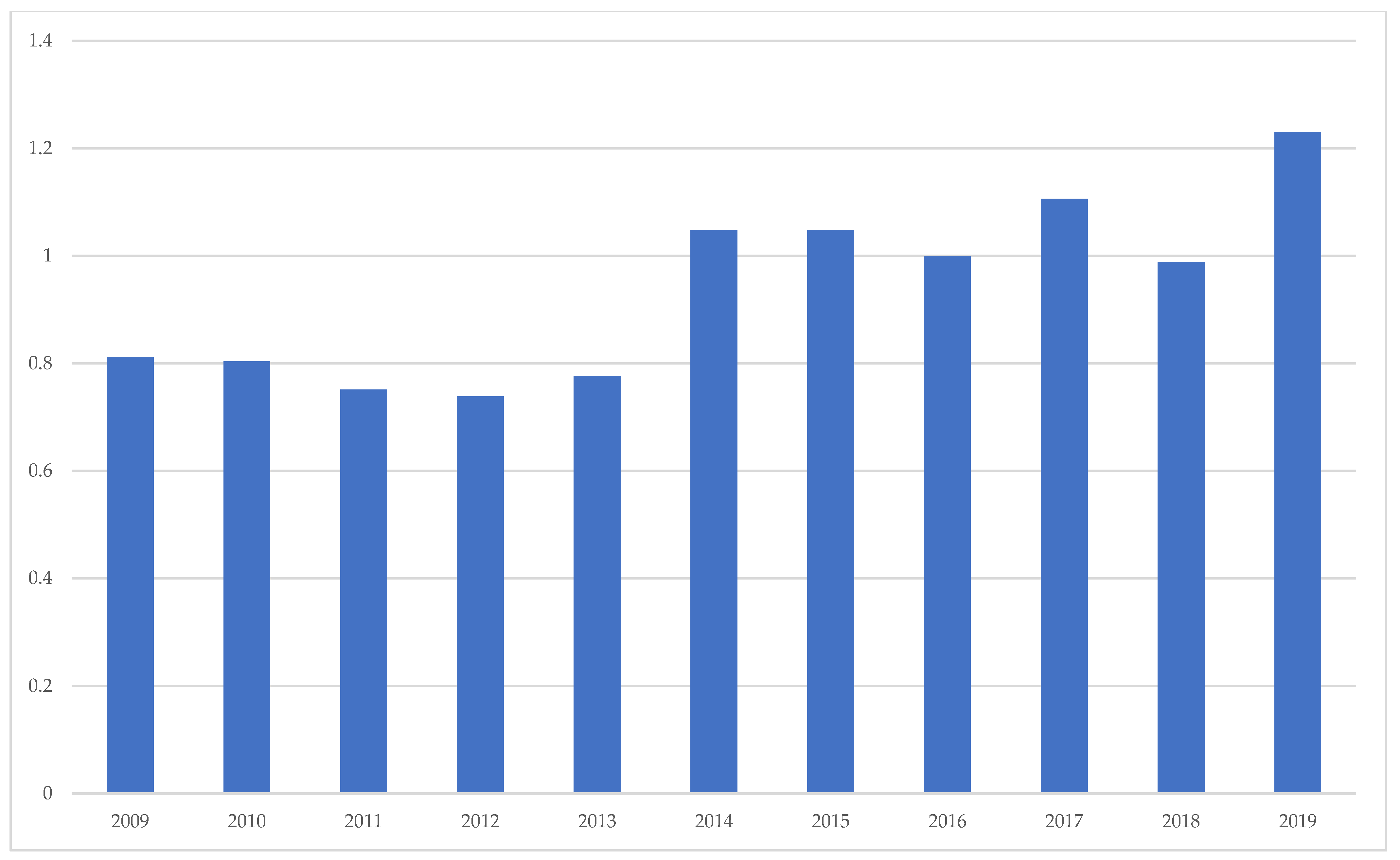
As the scale of sweet potato production has expanded over the years, the price of sweet potatoes has also experienced a gradual increase following the growth of the industry. As shown in Figure 3, the price of sweet potatoes was $0.81 per kg in 2009, and it increased to about $1.23 per kg in 2019. The increased unit price further suggests a growing demand for sweet potatoes [8,12,13].

2. Materials and Methods

The inverse demand models have been widely used in the literature to estimate the demand for perishable commodities, particularly fruit and vegetables [14,15]. In an inverse demand system, the quantities taken to the market are considered to be predetermined by the production because of perishability. Developed by Brown et al. [16], the Synthetic Inverse Demand System (SIDS), a model that nests four other inverse demand systems, will be employed in this study to examine how the sweet potato prices respond to changes in quantity. Starting with the consumer utility maximization problem, we have:

$$\max U\left(q\right) st.\sum p_i{q}_i=M$$

(1)

where $q$ is a vector of quantities for $i$ goods, $p$ is the vector of prices and the income is represented by $M$. The problem at Equation (1) produces the following two first-order conditions, where $\lambda$ is the Lagrange multiplier:

$$\begin{gathered} \sum p_i{q}_i=M \\ \frac{\partial U}{\partial p_i}=\lambda p_i \end{gathered}$$

Using the Wold’s identity, we obtain uncompensated inverse demand equations:

$$\frac{p_i}{M}=\frac{\frac{\partial U}{\partial q_i}}{{{\displaystyle \sum }}_j\left(\frac{\partial U}{\partial q_j}\right)q_j}\forall i\ne j \mathrm{and} i=1,\dots ,n.$$

Taking the dual of Equation (1) and rewriting the problem in terms of distance functions, we define $d\left(U,q\right)$ as the amount by which the quantity vector must be divided to reach the utility level $U$. Then, differentiating $d\left(\cdot \right)$ with respect to the quantities, we obtain a system of compensated inverse demands.

$$\frac{p_i}{M}=\frac{\partial d\left(U,q\right)}{\partial q_i}\equiv {\pi }_i\left(U,q\right).$$

(2)

Differentiating Equation (2) and a series of algebraic transformations yields the first demand system, the Rotterdam Inverse Demand System (RIDS) [17]:

$$w_{i}d\log \left({\pi }_i\right)=\left(w_i\frac{\partial \log \left({\pi }_i\right)}{\partial \log k}\right)\left[\sum w_{j}d\log \left(q_j\right)\right]+\sum \left(w_i\frac{\partial \log \left({\pi }_i\right)}{\partial \log \left(q_j\right)}\times \log \left(q_j\right)\right).$$

(3)

Here $k$ is a scalar and $w$ is the consumer’s budget share. We can define $d\log \left(Q\right)$ as $\sum w_{j}d\log \left(q_j\right)$, and also $h_i$ as $w_i\frac{\partial \log \left({\pi }_i\right)}{\partial \log k}$ and $h_{ij}$ as $w_i\frac{\partial \log \left({\pi }_i\right)}{\partial \log \left(q_j\right)}$. Adding $w_{i}d\log Q$ to both sides of Equation (3), we obtain the second system, the Laitinen and Theil Inverse Demand System (LTIDS):

$$w_i\left(d\log \left({\pi }_i\right)+d\log \left(Q\right)\right)=\left(w_i+h_i\right)d\log \left(Q\right)+\sum h_{ij}d\log \left(q_j\right).$$

(4)

Subsequently, Brown et al. [16] shows that by adding a specific term into Equation (4) and some other transformations, it is possible to obtain the Almost Ideal Inverse Demand System (AIIDS) [18]:

$${\mathit{dw}}_i=\left(w_i+h_i\right)d\log \left(Q\right)+{\displaystyle \sum }_j{\beta }_{\mathit{ij}}d\log \left(q_j\right).$$

(5)

where ${\beta }_{ij}$ can be treated as a parameter. Finally, if we subtract $w_{i}d\log \left(Q\right)$ from both sides of Equation (5), we obtain the fourth inverse demand system, specifically, the Rotterdam Almost Ideal Inverse Demand System (RAIIDS) that has the RIDS scale effects, and the AIIDS quantity effects:

$${\mathit{dw}}_i-w_{i}d\log \left(Q\right)=h_{i}d\log \left(Q\right)+\sum {\beta }_{\mathit{ij}}d\log \left(q_j\right).$$

(6)

At this point, Brown et al. (1995) follows the derivation of a synthetic demand system from Barten [19], which takes into account that the right-hand-side variables in models Equations (3)–(6) are the same, to obtain the SIDS after some reorganization of the variables:

$$w_{i}d\log \left({\pi }_i\right)=\left(c_i-d_1{w}_i\right)d\log \left(Q\right)+{\displaystyle \sum }_i\left(c_{ij}-d_2{w}_i\left({\delta }_{ij}-w_j\right)\right)d\log \left(q_j\right).$$

(7)

Here, ${\delta }_{ij}$ is the Kronecker-delta term that is equal to 1 if $i=j$, and zero otherwise; $c_i$ and $c_{ij}$ are the parameters to estimate. The above function meets the standard assumptions, such as adding-up, homogeneity, and symmetry, when ${{\displaystyle \sum }}_i{c}_i=-1+d_1$ and ${{\displaystyle \sum }}_i{c}_{ij}=0$, ${{\displaystyle \sum }}_j{c}_{ij}=0$, and $c_{ij}=c_{ji}$, respectively.

From Equation (7), it is possible to recover each one of the inverse demand systems nested in the synthetic model; i.e., when $d_1=d_2=0$, the RIDS model is identified, while if $d_1=d_2=1$, then the AIIDS model is identified. If $d_1=1$ and $d_2=0$, the LTIDS model is derived, and when $d_1=0$ and $d_2=1$, the RAIIDS model arises.

The flexibilities derived from Equation (7) are obtained in a very straightforward way. Taking the partial derivative of $\log \left({\pi }_i\right)$ with respect to $\log \left(Q\right)$ and $\log \left(q_j\right)$ will yield the scale and compensated quantity elasticities, respectively.

$${\epsilon }_i\equiv \frac{\partial \log \left({\pi }_i\right)}{\partial \log \left(Q\right)}=\frac{c_i-d_1{w}_i}{w_i}, and$$

(8)

$$f_{\mathit{ij}}\equiv \frac{\partial \log \left({\pi }_i\right)}{\partial \log \left(q_j\right)}=\frac{c_{\mathit{ij}}-d_2{w}_i\left({\delta }_{\mathit{ij}}-w_j\right)}{w_i}.$$

(9)

Furthermore, the uncompensated elasticity is obtained by combining Equations (8) and (9):

$$f_{ij}^{\ast }\equiv f_{ij}+w_i{\epsilon }_i.$$

(10)

In our analysis, the shipping point prices and market shares of sweet potatoes supplied by each state are used to create the dependent variable of Equation (7), while the quantities of sweet potatoes shipped by each state are used to compute the independent variables. Finally, the Divisia volume index is prepared via the sum of the market share multiplied by the respective quantity volume.

This study uses the price and quantity data of North Carolina, California, Mississippi, and Louisiana, obtained from the Agricultural Marketing Service (AMS) of the U.S. Department of Agriculture. The data of the exported quantity of sweet potatoes are from the database of USA Trade Online of the U.S. Census Bureau. The study uses the shipment volumes assigned to each state as the quantities of sweet potatoes, measured in million pounds. The price of sweet potatoes is presented by the prices at the shipping-point, measured in dollars per pound.

3. Results

The summary statistics of the price and quantity are shown in

Table 1. Descriptive statistics of the monthly data by source.

Variable	Country	Mean	Std. Dev.	Min	Max
Quantity	California	3.865	1.655	0.145	8.523
(million kilograms)	Louisiana	2.322	1.637	0.100	8.283
	Mississippi	4.285	2.110	0.163	13.154
	North Carolina	22.734	6.902	6.613	43.359
	Exports	11.554	7.415	1.947	31.076
Price	California	1.184	0.245	0.882	1.881
(dollars per kilogram)	Louisiana	1.001	0.117	0.827	1.296
	Mississippi	0.968	0.099	0.800	1.276
	North Carolina	0.880	0.086	0.745	1.237
	Exports	0.690	0.071	0.540	0.886

. As can be seen from Table 1 and Figure 1, North Carolina is in a dominant position in sweet potato production in the U.S. with the highest average quantity at 22.73 million kg. Following North Carolina are the states of Mississippi, California, and Louisiana, which have a total production of 4.29, 3.87, and 2.32 million kg, respectively. Sweet potato export accounted for about 11.55 million kg.

The prices of sweet potatoes from different markets vary and are consistent with the quantities in each state. Among the domestic suppliers, North Carolina has the lowest sweet potato price, at 0.88 dollars per kilogram, while other states have higher prices, averaged 1.18 dollars per kilogram. The study period is from January of 2009 to August of 2020. Shipment occurs in the U.S. all year round, with peak winter season including November and December. In addition, the variables are tested for unit roots, and we found no statistical evidence of unit roots in the variables.

The estimation results are presented in

Table 2. Estimated parameters for the synthetic inverse demand system.

			Price Parameters
	Nesting Parameters	Scale Parameters	California	North Carolina	Mississippi and Louisiana	Exports
California		−0.005 (0.004)	0.001 (0.001)	−0.003 (0.002)	−0.003 (0.001)	0.004 (0.003)
North Carolina		0.041 (0.014)		0.018 (0.008)	0.012 (0.003)	0.033 (0.012)
Mississippi and Louisiana		0.014 (0.005)			−0.003 (0.001)	0.018 (0.004)
Exports		0.021 (0.006)				−0.055 (0.016)
$d_1$	1.071 (0.027)
$d_2$	0.084 (0.022)
Log-likelihood	1211.566

Note: Standard error in parenthesis.

. The export equation, its parameters, and its standard deviations are recovered via the adding-restrictions. The log-likelihood value is 1211.6, and the estimates $d_1$ and $d_2$ from Equation (7) are 1.071 and 0.084, respectively, which means that the SIDS model is statistically different from all other individual models, but it is close to the Laitinen-Theil model. The same situation occurred in the strawberry model estimated by Suh et al. [14].

Table 3. Log-likelihood of nested systems, and comparison with the synthetic inverse demand system.

System	d1	d2	LL Value	LR Test
RIDS	0	0	959.674	503.783
LTIDS	1	0	1204.639	13.854
AIIDS	1	1	909.436	604.261
RAIIDS	0	1	775.204	872.724

Note: RIDS: Rotterdam Inverse Demand System; LTIDS: Laitinen-Theil Inverse Demand System; AIIDS: Almost Ideal Inverse Demand System; RAIIDS: Rotterdam Almost Ideal Inverse Demand System.

reports the results of the log-likelihood (LL) value and the log-likelihood ratio (LR) for each individual model and for the nested model. The LR test can be used to compare the individual models with the SIDS model. If the LR test value is positive, it indicates that the individual model is rejected in favor of the nested one, which is what happens in this case, because all of the LR tests are positive. The SIDS model is chosen to compute the flexibilities of the sweet potato market.

3.1. Scale Elasticity

All estimates are negative and statistically significant at 1% (

Table 4. Elasticities and price flexibilities for the synthetic inverse demand system.

		Price Flexibilities
	Scale Flexibilities	California	North Carolina	Mississippi and Louisiana	Exports
California	−1.117 (0.023)	−0.197 (0.025)	−0.560 (0.016)	−0.196 (0.007)	−0.163 (0.027)
North Carolina	−0.993 (0.008)	−0.112 (0.003)	−0.593 (0.024)	−0.177 (0.003)	−0.111 (0.025)
Mississippi and Louisiana	−0.986 (0.008)	−0.121 (0.004)	−0.540 (0.009)	−0.257 (0.023)	−0.068 (0.025)
Exports	−0.959 (0.023)	−0.081 (0.015)	−0.284 (0.065)	−0.055 (0.022)	−0.538 (0.100)

Note: Standard errors in parenthesis.

), meaning that an increase in the quantity will decrease the price of sweet potatoes. Specifically, a 1% increase in the aggregate shipment of sweet potatoes will decrease the prices of the California, North Carolina, the aggregate Mississippi and Louisiana, and exports by 1.12%, 0.99%, 0.99%, and 0.96%, respectively. When these values are evaluated at sample prices and quantities, we know that a 1% increase in the monthly shipment will decrease the price by 0.6, 0.4, 0.44, and 0.3 cents per kilogram for California, North Carolina, Mississippi-Louisiana, and export.

3.2. Price Flexibility: Own-Price

The own-price flexibility is in the diagonal of Table 4. North Carolina has a higher own-price flexibility of −0.59, meaning that a 1% increase in its own shipment will decrease its price by 0.59%. When evaluated at the sample mean, North Carolina price will decrease 5.2 cents per kilogram for an increase of 5 million kilograms. Additionally, one percent of increase in the own shipment will decrease the prices of California, Mississippi-Louisiana, and exports by 0.20%, 0.26%, and 0.54%, respectively. Evaluated at the mean, it implies that when the own monthly shipment increases by 5 million kilograms, the prices will decrease by 13.7, 8.6, and 7.3 cents per kilogram, respectively, for these players.

3.3. Price Flexibility: Cross-Price

The cross-price flexibilities are all negative and statistically significant at the 1% level. It is clear that North Carolina has a major impact over the market. An increase of 1% from this state will lead to a decrease in the prices for California, Mississippi-Louisiana, and exports by 0.56%, 0.54%, and 0.28%, respectively. Evaluated in the sample mean, when North Carolina increases its monthly shipments by 5 million kilograms, it will decrease the prices by 6.6, 5.2, and 1.9 cents per kilogram respectively for the these players. When California increases 1% of its shipments, it will decrease the prices of North Carolina, Mississippi-Louisiana, and exports by 0.11%, 0.12%, and 0.08%, respectively. When Mississippi-Louisiana does the same, the price decreases by 0.20%, 0.18%, and 0.06% for California, North Carolina, and exports, respectively. When evaluated at the sample mean, an increase in the California monthly shipment by 5 million kilograms, the price of North Carolina, Mississippi-Louisiana, and exports will decrease by 5.7, 6.9, and 3.2 cents per kilogram, respectively. Additionally, for the case of Mississippi-Louisiana, the prices will decrease by 7.9, 5.3, and 1.3 cents for California, North Carolina, and exports, respectively.

3.4. Scenario Analysis

As the sweet potato industry in the United States is led by North Carolina, the effect of diseases in this state can have a significant impact on the market. This section simulates the effect of changes in the North Carolina supply under different scenarios. Specifically, we evaluate increases and decreases in the NC supply of 25% and 50%. To do this, we take the point estimates of the flexibilities and the average shares per state or region. In the Appendix A, detailed changes in prices and revenues for each scenario and each state are presented according to month. It should be pointed out that this simulation is based on a static analysis of the market, assuming that other variables remain unchanged.

Table 5. Summary of changes in sweet potato shipment values under four scenarios.

	Scenario	California		Mississippi and Louisiana		Exports		North Carolina
		($ Million)	(%)	($ Million)	(%)	($ Million)	(%)	($ Million)	(%)
Value	Baseline	58.83		36.27		135.48		248.13
	25% NC increase	51.04		31.61		126.85		265.27
	50% NC increase	43.26		26.95		118.22		264.45
	25% NC decrease	66.61		40.93		144.12		213.03
	50% NC decrease	74.39		45.58		152.75		159.98
Total losses	25% NC increase	7.78	15.2%	4.66	14.7%	8.63	6.8%	17.14 *	6.5% *
	50% NC increase	15.57	36.0%	9.32	34.6%	17.26	14.6%	16.32 *	6.2% *
Total gain	25% NC decrease	7.78	11.7%	4.66	11.4%	8.63	6.0%	35.10 #	16.5% #
	50% NC decrease	15.57	20.9%	9.32	20.4%	17.26	11.3%	88.15 #	55.1% #

Note. *: In the North Carolina case, an increase will produce a gain. ^#: In the case of North Carolina, a decrease in the supply will produce a loss.

shows a summary of the total effect for each scenario and each player, when North Carolina increases or decreases the supply. In general, it is observed that the effect in all states is large, suggesting high sensitivities to what happens in North Carolina. Specifically, a 25% increase in NC would lead to a loss of 15.2%, 24.7%, and 6.8% for California, Mississippi-Louisiana, and exports, respectively. However, although the price falls, the quantity increase by NC results in an overall revenue increase of 6.5%. When we evaluate the effect of a 50% increase in NC’s supply, the losses for other players are even greater. California and Mississippi-Louisiana would lose 36.0% and 43.6%, respectively. This increase would not result in further revenue gains for NC, since the decrease in price produced only an increase of 6.2% of its revenue, which is slightly less when compared with the 25% supply increase scenario.

When North Carolina reduces its supply, the shipment value of the rest of the producers increases, with California, Mississippi-Louisiana, and exports increasing by 11.7%, 11.4%, and 6%, respectively, under the 25% reduction scenario, and by 20.9%, 20.4%, and 11.3% under the 50% reduction scenario. For NC itself, it would lose 16.5% and 55.1% when its supply drops by 25% and 50% (monthly changes of this simulation are presented in

Table A1. Effects of North Carolina supply changes on monthly prices and shipment values of sweet potatoes.

State	Month	Baseline			25% Increase		50% Increase		25% Decrease		50% Decrease
		Quantity	Price	Value	Price	Reduced Value	Price	Reduced Value	Price	Reduced Value	Price	Reduced Value
		(Million kgs)	($/kg)	($ Million)	($/kg)	($ Million)	($/kg)	($ Million)	($/kg)	($ Million)	($/kg)	($ Million)
California	1	4.02	1.21	4.91	1.06	4.26	0.90	3.61	1.39	5.57	1.54	6.22
	2	4.49	1.23	5.58	1.08	4.83	0.90	4.08	1.41	6.34	1.59	7.09
	3	4.58	1.26	5.74	1.10	5.03	0.95	4.31	1.41	6.46	1.57	7.18
	4	3.44	1.23	4.25	1.08	3.74	0.95	3.23	1.39	4.76	1.52	5.28
	5	3.66	1.28	4.70	1.12	4.09	0.95	3.48	1.46	5.31	1.61	5.93
	6	3.13	1.32	4.17	1.17	3.63	0.99	3.09	1.50	4.71	1.68	5.25
	7	2.00	1.21	2.41	1.04	2.06	0.86	1.72	1.37	2.75	1.54	3.10
	8	1.32	1.70	2.24	1.46	1.92	1.21	1.61	1.94	2.56	2.16	2.87
	9	3.42	1.57	5.37	1.37	4.65	1.15	3.93	1.79	6.09	1.98	6.80
	10	3.95	1.41	5.54	1.21	4.77	1.01	4.00	1.59	6.31	1.79	7.08
	11	7.14	1.21	8.67	1.06	7.52	0.88	6.36	1.37	9.83	1.54	10.98
	12	4.34	1.21	5.23	1.04	4.53	0.88	3.83	1.37	5.93	1.52	6.63
Mississippi	1	2.83	1.01	2.90	0.88	2.53	0.75	2.15	1.15	3.27	1.28	3.65
and Louisiana	2	2.66	1.01	2.69	0.88	2.34	0.75	1.99	1.15	3.05	1.28	3.40
	3	3.07	0.99	3.07	0.88	2.70	0.75	2.32	1.12	3.44	1.23	3.81
	4	3.09	0.99	3.06	0.88	2.70	0.75	2.34	1.10	3.41	1.21	3.77
	5	2.80	1.01	2.82	0.88	2.46	0.75	2.11	1.12	3.18	1.26	3.53
	6	2.65	1.01	2.71	0.90	2.37	0.77	2.03	1.15	3.05	1.28	3.40
	7	2.54	0.97	2.48	0.84	2.14	0.71	1.80	1.12	2.83	1.26	3.17
	8	2.83	1.04	2.91	0.88	2.52	0.75	2.12	1.17	3.31	1.30	3.70
	9	1.94	1.08	2.09	0.95	1.82	0.79	1.55	1.21	2.36	1.37	2.63
	10	2.16	1.06	2.26	0.90	1.96	0.77	1.66	1.19	2.57	1.32	2.87
	11	5.04	1.01	5.14	0.88	4.48	0.75	3.82	1.15	5.80	1.28	6.46
	12	3.97	1.04	4.13	0.90	3.59	0.77	3.06	1.17	4.66	1.30	5.19
Exports	1	20.58	0.64	13.33	0.60	12.47	0.57	11.60	0.68	14.19	0.73	15.06
	2	23.80	0.64	15.41	0.60	14.39	0.55	13.36	0.68	16.44	0.73	17.47
	3	24.76	0.66	16.60	0.64	15.64	0.60	14.68	0.71	17.56	0.75	18.51
	4	23.53	0.64	14.94	0.60	14.13	0.57	13.32	0.66	15.74	0.71	16.55
	5	21.11	0.66	14.11	0.62	13.23	0.60	12.35	0.71	14.99	0.75	15.87
	6	17.15	0.68	11.79	0.64	11.06	0.60	10.33	0.73	12.52	0.77	13.25
	7	11.16	0.68	7.58	0.64	7.02	0.57	6.46	0.73	8.14	0.77	8.70
	8	10.18	0.62	6.21	0.57	5.76	0.53	5.31	0.66	6.65	0.71	7.10
	9	5.70	0.64	3.70	0.60	3.45	0.57	3.21	0.68	3.94	0.73	4.18
	10	14.23	0.64	8.98	0.60	8.35	0.55	7.72	0.68	9.60	0.73	10.23
	11	17.57	0.64	11.28	0.60	10.54	0.55	9.81	0.68	12.01	0.73	12.74
	12	17.74	0.66	11.57	0.62	10.82	0.57	10.06	0.71	12.33	0.73	13.09
North	1	25.06	0.84	20.93	0.71	22.39	0.60	22.33	0.95	17.96	1.08	13.49
Carolina	2	26.10	0.84	21.58	0.71	23.13	0.60	23.14	0.95	18.49	1.06	13.86
	3	31.90	0.84	26.63	0.71	28.24	0.57	27.83	0.97	23.00	1.08	17.36
	4	27.33	0.84	22.80	0.71	24.07	0.57	23.56	0.97	19.76	1.10	14.95
	5	24.56	0.84	20.51	0.71	21.88	0.60	21.74	0.95	17.64	1.08	13.27
	6	20.46	0.84	17.25	0.73	18.38	0.60	18.25	0.97	14.84	1.08	11.16
	7	19.45	0.88	17.12	0.77	18.51	0.64	18.76	0.99	14.57	1.12	10.86
	8	18.24	0.86	15.58	0.73	16.81	0.62	16.97	0.97	13.29	1.08	9.92
	9	12.82	0.97	12.56	0.84	13.45	0.71	13.44	1.12	10.77	1.26	8.08
	10	21.10	0.90	19.28	0.79	20.75	0.66	20.87	1.04	16.47	1.17	12.32
	11	35.42	0.88	31.58	0.77	33.79	0.64	33.71	1.01	27.10	1.15	20.34
	12	25.90	0.86	22.30	0.73	23.87	0.62	23.84	0.99	19.13	1.10	14.36

, in the Appendix A).

3.5. Discussion

This study analyzes the sweet potato price response when the market supply changes and simulates the effects of major supply shocks with different intensities. In the literature, simulation studies have been conducted with respect to regular potatoes, another major type of root vegetable that may provide an interesting comparison. Using an agent-based modeling approach, Rahman et al. [20] finds that if climatic shocks were to affect regular potato supplies in Idaho, the largest producer of potatoes in the U.S., the price of potatoes would spike, which would lead consumers to prefer processed potato products. Our simulation results indicate that if there is a shock that affects sweet potato production in North Carolina, the decrease in the supply of sweet potatoes will produce not only a price increase, but also an increase in the shipment value of sweet potatoes from other states.

Our results suggest that the high level of geographic concentration of U.S. production in the state of North Carolina means that the U.S. market will be significantly affected if that state suffers a shock. Thus, policies that would motivate geographic diversification would make sweet potato production more sustainable and less sensitive to shocks.

4. Conclusions

This study uses the Synthetic Inverse Demand System model to examine the price dynamics of sweet potatoes among the major producing states and exports market, and to evaluate how shocks in supply that could arise from a disease outbreak or a weather event would affect market prices and economic outcomes. The model accounts for the linkage between the prices and quantities of different markets and estimates sweet potato market price responses. This study is the first research that provides empirical evidence for the dynamics of sweet potato prices in the U.S. market.

The changes in the total production in North Carolina, California, Mississippi, and Louisiana, as well as the exporting sector, not only affect their own sweet potato prices, but also impact on other states. Because of its dominating position in sweet potato production, the changes in the total production of North Carolina are found to have the greatest impact on sweet potato prices. An increase of 5 million kilograms in monthly sweet potato shipment in North Carolina would reduce the prices in California, Mississippi-Louisiana, and exports by 6.6, 5.2, and 1.9 cents per kilogram, respectively.

This study sheds light on how prices respond to quantity changes in the U.S. market. The information is essential for economic analysis and policymaking in the industry. The results of this research point toward the importance of having a stable supply of sweet potatoes, particularly in North Carolina, which produces over half of the sweet potatoes in the U.S. Given the dynamics of sweet potato prices and quantities across different markets in the U.S., the effort to tackle potential challenges that may introduce risks into sweet potato production is crucial and merits the attention of policymakers.

Although our model is general, as it nests four demand systems (SIDS), future research could benefit from testing other forms of demand models. The simulation offered in this research considers the changes in the market when there is a shock on supply. In future works, more complex simulations could be carried out to include multiple products and interactions between products.