Prediction of Technological Maturity of Grapevines Under a Double Pruning System Using Data Fusion and Machine Learning

Abstract

The production of “winter wines” in south-eastern Brazil, enabled by the double pruning technique, requires precise assessment of grape technological maturity to ensure high-quality outputs. However, conventional monitoring approaches are destructive, labor-intensive, and limited in their ability to capture vineyard spatial variability. This study aimed to develop and validate a non-destructive predictive framework for Soluble Solids (°Brix) and Titratable Acidity (TA) by integrating spatial remote sensing data with temporal agrometeorological information. Multispectral imagery was acquired via an unmanned aerial vehicle in a vineyard cultivated with Sauvignon Blanc and Syrah, from which vegetation indices were derived and combined with Growing Degree-Days to train machine learning models, including Random Forest, Multilayer Perceptron, and XGBoost. The incorporation of agrometeorological data significantly improved predictive performance compared to models based solely on vegetation indices. Among the tested algorithms, XGBoost achieved the highest accuracy, with coefficients of determination of 0.89 for °Brix and 0.77 for TA, achieved by XGBoost on an independent hold-out test set. Model interpretability analysis indicated that Growing Degree-Days and cultivar were the primary drivers of maturation dynamics, while vegetation indices refined predictions by accounting for spatial variability in plant vigor. Overall, the proposed approach represents a promising proof-of-concept framework for non-destructive maturity monitoring in precision viticulture, supporting improved monitoring of grape maturation. However, multi-season validation across diverse vineyard conditions is required to confirm its generalizability and support its application as a routine decision-support tool.

1. Introduction

Global viticulture has witnessed the emergence of new production regions that employ innovative management techniques to achieve high-quality wines in climates previously considered marginal. A notable example is the production of “winter-harvest wines” in southeastern Brazil, made possible by the double pruning technique. This practice inverts the grapevine’s harvest cycle to the dry winter period, promoting the concentration of sugars and phenolic compounds in the berries [1]. The success of this and other viticultural practices fundamentally depends on the ability to precisely determine the optimal harvest time, a point defined by the concept of technological maturity. This stage represents the ideal balance between sugars, measured as Soluble Solids (°Brix), and Titratable Acidity (TA), parameters that directly govern the wine’s alcoholic potential, stability, and sensory profile [2].

Accurately determining the harvest point is a decisive factor in viticulture, as the quality of the grapes at the time of picking directly influences the potential of the final wine [3]. Traditionally, monitoring relies on manual berry sampling and laboratory analysis, a destructive, time-consuming, and spatially limited approach that fails to capture within-vineyard variability in maturity, potentially leading to suboptimal harvest decisions [4]. To overcome these limitations, precision viticulture has emerged as a promising field employing remote sensing technologies for non-destructive, large-scale monitoring. Unmanned Aerial Vehicles (UAVs) equipped with multispectral sensors have become a powerful tool for assessing the spatial variability of the vegetative canopy [5], from which Vegetation Indices (VIs) are calculated as proxies for plant vigor, nutritional status, and water status [6]. However, VIs correlate inconsistently with grape quality parameters [7], as canopy vigor does not always directly translate to fruit maturation due to complex mediating factors such as water balance and source–sink relationships.

This reveals a fundamental gap: VIs provide a spatial snapshot of plant condition but lack the temporal dimension needed to capture phenological development. Studies using VIs as sole predictors have reported limited accuracy, with maximum R² values of 0.52 [8] and 0.61 [9] for Brix prediction, confirming that spatial vigor information alone cannot represent the cumulative, thermally driven nature of ripening. Growing Degree-Days (GDD), a well-established agrometeorological indicator that quantifies the accumulated thermal energy required for phenological stage transitions [10], offers a complementary temporal dimension. GDD-based approaches combined with machine learning have proven effective for predicting growth and yield in crops such as rice and sweet potato [11,12]; however, the synergistic integration of spatial (VIs) and temporal (GDD) data for grapevine technological maturity prediction remains a largely unexplored area.

The central hypothesis of this work is that fusing spatial (VIs) and temporal (GDD) predictors through machine learning models can overcome the limitations of individual approaches, generating more accurate and robust estimates of technological maturity. Therefore, the objective of this study was to develop and assess machine learning models for the non-destructive prediction of Soluble Solids (°Brix) and Titratable Acidity in ‘Sauvignon Blanc’ and ‘Syrah’ grapes grown under a double pruning regime. The specific objectives were: (i) to investigate whether the inclusion of GDD as a predictor variable significantly improves the accuracy of VI-based models; (ii) to identify the most influential VIs for predicting grape maturity; and (iii) to determine the best-performing machine learning algorithm for this task.

2. Materials and Methods

2.1. Study Area

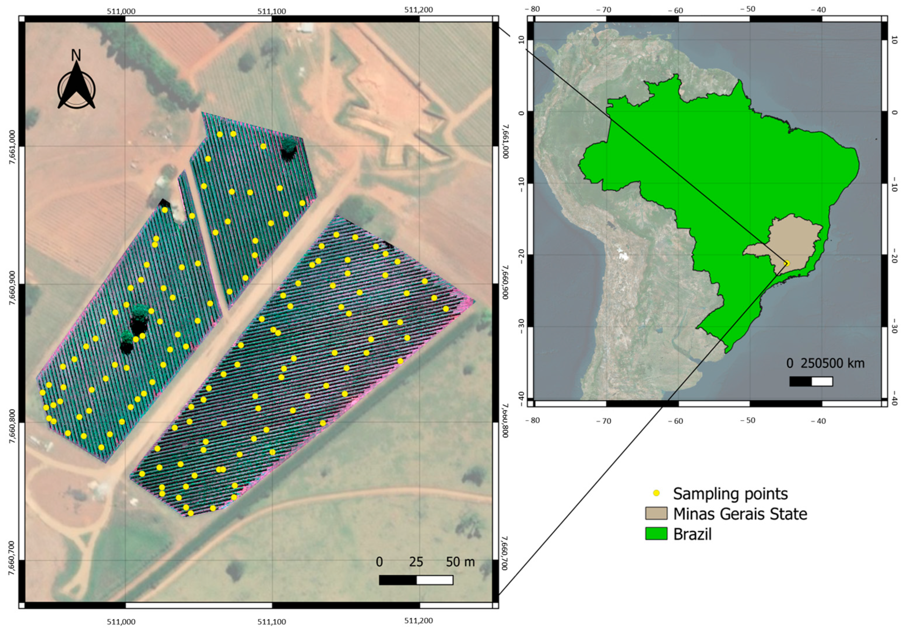
The experiment was conducted during the 2024 winter harvest cycle, which commenced with production pruning in January 2024 and concluded with harvest in the winter (July/August) of 2024. The study area is a commercial Vitis vinifera vineyard located in the Macaia district, municipality of Bom Sucesso, Minas Gerais, Brazil. The area is situated at the geographical coordinates 21°9′12.78″ S and 44°53′36.45″ W, at an average altitude of 952 m (Figure 1). The local topography features an average slope of 13%. According to the Köppen–Geiger classification, the regional climate is classified as Cwa (humid subtropical with a dry winter and hot summer) [13], with an average temperature of the warmest month exceeding 22 °C.

2.2. Vineyard Details

The experimental area covers 4.54 hectares, divided into two commercial blocks composed of two Vitis vinifera L. cultivars: ‘Sauvignon Blanc’ (white) and ‘Syrah’ (red). Both cultivars were grafted onto the ‘IAC 766’ rootstock.

The vineyard was established in 2021, with the vines being in their third year (third leaf) during the experimental cycle. The vines are trained on a vertical shoot positioning (VSP) trellis system. The blocks feature distinct row orientations: one aligned Northeast–Southwest and the other Northwest–Southeast. Planting spacing is 1 m between vines and 2.6 m between rows, resulting in a density of 3846 vines per hectare. Management for the winter cycle was initiated with production pruning carried out in January 2024, following the double pruning system [1]. The vineyard is equipped with a drip irrigation system for supplemental watering.

2.3. Sampling Design and Field Data Collection

To monitor ripening progression, 145 georeferenced sampling points were defined within the experimental area. Data collection was carried out during the grape ripening phase, commencing after the onset of veraison.

The 145 georeferenced sampling points were distributed across both cultivar blocks in proportion to their respective areas, with 70 points located in the ‘Sauvignon Blanc’ block and 56 points in the ‘Syrah’ block. Over six collection dates, this design generated a total dataset of 870 individual observations (145 points × 6 dates). No formal statistical outlier removal procedure was applied to the physicochemical data; samples compromised by berry damage or equipment malfunction during laboratory analysis were excluded on a case-by-case basis and replaced where feasible.

The final analytical dataset comprised 494 observations from 126 georeferenced sampling points over five collection dates. Descriptive statistics for the response variables were: Soluble Solids ranged from 7.6 to 21.7 °Brix (mean = 16.6 ± 2.87 °Brix; CV = 17.3%); Titratable Acidity ranged from 4.1 to 24.7 g/L (mean = 11.15 ± 4.46 g/L; CV = 40.0%).

Collections occurred on six consecutive dates in 2024 (14 June, 18 June, 26 June, 4 July, 10 July, and 17 July), at approximately weekly intervals leading to harvest. At each sampling point and on each date, 20 grape berries were manually harvested. The sampling was stratified, with berries collected from three distinct vertical positions within the grape clusters (top, middle, and bottom) and evenly distributed across both sides of the vertical shoot-positioned (VSP) trellis system. Samples were immediately placed in labeled plastic bags and transported under refrigeration.

2.4. Physicochemical Analysis (Technological Maturity)

Samples were processed at the Fruit Science Laboratory of the Federal University of Lavras (UFLA). The 20 berries from each point were homogenized and gently crushed manually to prevent seed damage. The resulting juice (must) was filtered and subjected to analysis of the following physicochemical parameters:

• Soluble Solids (SS): SS content was determined using a calibrated digital refractometer, with results expressed in °Brix.
• Titratable Acidity (TA): Total acidity was quantified following the standardized Adolf Lutz protocol [14]. The results were subsequently converted and expressed as tartaric acid equivalents (g/L) to ensure methodological consistency and comparability.

2.5. Multispectral Image Acquisition, Processing and Analysis

Multispectral image acquisition was performed on six dates throughout the ripening cycle, coinciding with the field sampling days. All flights were conducted between 11:00 AM and 1:00 PM (local time, UTC-3) under clear-sky conditions to ensure consistent solar illumination. An Unmanned Aerial Vehicle (UAV), model Mavic 3M (DJI, Shenzhen, China), was used. It was equipped with a Real-Time Kinematic (RTK) georeferencing system, aided by a D-RTK 2 base station (DJI, Shenzhen, China), to ensure high positional accuracy. The onboard multispectral sensor features four spectral bands: Green (G) (560 ± 16 nm), Red (R) (650 ± 16 nm), RedEdge (RE) (730 ± 16 nm), and Near-Infrared (NIR) (860 ± 26 nm).

Flight missions were planned and executed using DJI Pilot 2 software at an altitude of 80 m. Flight parameters included a speed of 5 m/s and 80% frontal and lateral overlap to ensure proper orthomosaic generation. Photogrammetric processing was performed using Pix4Dmapper v. 4.8.4 (Pix4D SA 2025). The images from each flight were imported into individual projects using the RTK metadata. Processing followed the ‘Ag Multispectral’ template, which includes image alignment, dense point cloud generation, and, finally, orthomosaic generation.

Radiometric calibration was applied during processing to convert Digital Number (DN) values to surface reflectance. To achieve this, images of a standard reflectance panel, captured on the ground before each flight, were imported and used by the software’s calibration tool, ensuring data comparability across the different dates. At the end of processing for each date, multispectral reflectance orthomosaics were generated, containing all four bands (G, R, RE, NIR) with a final spatial resolution of 4.2 cm. The files were exported in GeoTIFF format using the WGS 84/UTM Zone 23S coordinate system.

The calibration panel used was the MicaSense Multispectral Calibration Reflectance Panel with nominal per-band reflectance values of 48.9% (Green, 560 nm), 48.9% (Red, 650 nm), 48.8% (RedEdge, 730 nm), and 48.6% (NIR, 860 nm) as specified in the manufacturer’s calibration reference (RP06-2051010-OB, MicaSense). Calibration certificates are available upon request from the corresponding authors. Regarding per-flight meteorological conditions, all flights were conducted under clear-sky conditions.

All post-processing and image analysis steps were conducted in the R software environment v. 4.1.1 [15], supported by the ‘terra’ v. 1.8.70 [16], ‘sf’ v. 1.0.21 [17], and ‘FIELDimageR’ v. 0.6.2 [18] packages. First, to ensure perfect pixel-to-pixel overlap between collection dates, temporal co-registration of the six images was performed, aligning all orthomosaics to the image from the first flight date. Next, vegetation segmentation was carried out to remove soil pixels. A supervised classification method using the Random Forest (RF) algorithm was employed. Training polygons were manually digitized over representative ‘canopy’ and ‘soil’ areas using tools from the FIELDimageR v. 0.6.2 package [18]. From these, 400 random sample points per class were used to train the classifier using the superClass function from the ‘RStoolbox’ 1.0.2.2 package [19]. The resulting classification map was then used as a mask to extract exclusively vegetation pixels for subsequent analyses.

2.6. Feature Selection

The feature selection pipeline consisted of two sequential stages, aiming to obtain a subset of predictors that were both relevant (RFE) and independent (VIF). The entire process was conducted in the Python language v 3.9 using the scikit-learn library.

Given the large number of existing Vegetation Indices (VIs), 20 VIs were initially calculated. The first selection stage employed Recursive Feature Elimination (RFE) [20]. RFE is a wrapper technique that uses an external estimator, in this case, the Random Forest Regressor [21], to iteratively rank predictor importance. The estimator was configured with 100 trees (n_estimators = 100) and a fixed random state (random_state = 42) for reproducibility. The RFE was executed independently for the target variables Soluble Solids (°Brix) and Titratable Acidity (g/L), following the removal of samples with missing target data and median imputation of missing predictors. The algorithm was set to select the subset containing the 10 most important features for each target, generating two preliminary lists of VIs.

To ensure model stability and remove predictor redundancy, the two 10-VI subsets generated by RFE were subjected to Variance Inflation Factor (VIF) analysis. The VIF was calculated for all variables in each subset. In an iterative process, the variable with the highest VIF value was identified; if this value was greater than 5, the feature was removed. The VIF was then recalculated for the remaining variables. This process was repeated until all VIs in the subset exhibited a VIF value below 5. This resulted in a final set of low-collinearity VIs for each target variable, which was then effectively used in the modeling stage.

2.7. Selected Vegetation Indices for Modeling

At the conclusion of the feature selection pipeline (RFE followed by VIF), the final sets of predictors for each target variable were defined. The process resulted in the selection of five Vegetation Indices (VIs) for the Soluble Solids (°Brix) model and five VIs for the Titratable Acidity (g/L) model. These two predictor sets were effectively used as inputs for the modeling stage. The details, mathematical equations, and original bibliographical references for each of these selected VIs are presented in

Table 1. Vegetation Indices (VIs) selected as predic.tors for the Soluble Solids (°Brix) and Titratable Acidity (TA) models, their mathematical equations, and original references.

Index	Equation	Reference
Burn Area Index (BAI)	${\displaystyle \frac{1}{{\left(0.1-Red\right)}^2+{(0.06-NIR)}^2}}$	[22]
Spectral Feature Depth Vegetation (SFDVI)	${\displaystyle \frac{Green+NIR}{2}}-{\displaystyle \frac{Red+RedEdge}{2}}$	[23]
Green Difference Vegetation Index (GDVI)	$NIR-Green$	[24]
Chlorophyll Vegetation Index (CVI)	$NIR\times {\displaystyle \frac{Red}{{Green}^2}}$	[25]
Transformed Soil-Adjusted Vegetation Index (TSAVI)	${\displaystyle \frac{1.2\times (NIR-1.2\times Red-0.04)}{1.2\times NIR+Red-1.2\times 0.04+0.08\times (1+{1.2}^2)}}$	[26]
Plant Senescence Reflectance Index (PSRI)	${\displaystyle \frac{Red-Green}{RedEdge}}$	[27]
Transformed chlorophyll absorption in reflectance (TCARI)	$3\times (\left( RedEdge-Red\right)-0.2)\times \left(RedEdge-Green\right)\times ({\displaystyle \frac{RedEdge}{Red}})$	[28]

.

2.8. Growing Degree Days (GDD)

To quantify thermal accumulation during the experimental cycle, Growing Degree-Days (GDD) were calculated. Daily maximum (Tmax) and minimum (Tmin) air temperature data were obtained for the experiment’s location from the NASA POWER platform [29].

Daily GDD was calculated using the methodology proposed by Villa Nova [10], which accounts for various scenarios where minimum temperatures may fall below the base temperature (Tb). A Tb of 10 °C was adopted, which is the standard for grapevine (Vitis vinifera). The equations used were:

$$\mathrm{If} \mathrm{Tm} > \mathrm{Tb}: GOD={\displaystyle \frac{(TM+Tm)}{2}}-Tb$$

(1)

$$\mathrm{If} \mathrm{Tm} < \mathrm{Tb} < \mathrm{TM}: GOD={\displaystyle \frac{{(TM+Tb)}^2}{2\times (TM-Tm)}}$$

(2)

$$\mathrm{If} \mathrm{TM} < \mathrm{Tb}: GOD=0$$

(3)

where GDD represents the accumulated Growing Degree-Days (degrees °C × day) from the production pruning date to the respective field collection date; Tmax and Tmin are the daily maximum and minimum air temperatures (degrees °C), respectively; Tb is the base temperature, set at 10 degrees C for Vitis vinifera [10]; and n represents each individual day in the accumulation period.

GDD was accumulated daily, with the summation starting from the production pruning date. The cumulative GDD value from this start date until each respective field sampling date was then used as a predictor variable in the machine learning models.

2.9. Models

Three machine learning algorithms were selected to represent methodologically distinct paradigms: Random Forest (RF), a bagging ensemble of decision trees recognized for its robustness and built-in feature importance estimation [21]; XGBoost (XGB), a gradient-boosting framework with demonstrated superiority on structured tabular data; and Multi-layer Perceptron (MLP), a feedforward neural network capable of capturing complex non-linear relationships. This selection enables cross-paradigm benchmarking while covering the principal algorithmic approaches applied in precision agriculture. The categorical variable ‘Cultivar’ (Sauvignon Blanc/Syrah) was binary-encoded (0 = Sauvignon Blanc; 1 = Syrah) prior to model training. Feature standardization (mean = 0; standard deviation = 1) using StandardScaler was applied exclusively to the continuous predictors (the five selected VIs and, in the data fusion scenario, GDD); the binary cultivar encoding was excluded from standardization to preserve its categorical interpretation.

To predict the maturity variables (°Brix and Titratable Acidity), the optimized VI subsets were used as input for three machine learning algorithms: Random Forest (RF), XGBoost (XGB), and Multi-layer Perceptron (MLP). The workflow followed three stages: data preparation, hyperparameter optimization, and final evaluation.

First, the dataset was split into two subsets: 70% for training and 30% for testing (hold-out). The split was stratified by the ‘Cultivar’ variable to ensure representativeness in both sets. Next, the predictors in the training set were standardized (mean: 0, standard deviation: 1) using the StandardScaler. The scaling parameters derived from the training set were then applied to the test set, preventing data leakage.

To find the optimal hyperparameter combination for each algorithm, GridSearchCV was employed, combined with 5-fold cross-validation, applied exclusively to the training set (70%).

Table 2. Hyperparameter search space (optimization grid) explored via Grid Search for the Random Forest (RF), XGBoost (XGB), and Multi-layer Perceptron (MLP) algorithms.

Model	Hyperparameter	Values
Random Forest (RF)	n_estimators	100, 200, 300
	max_depth	None, 10, 20
	min_samples_split	2, 5
	min_samples_leaf	1, 2
	max_feautures	‘sqrt’, ‘log2’
XGBoosting (XGB)	n_estimators	100, 200, 300
	learning_rate	0.05, 0.1
	max_depth	3, 5
	subsample	0.7, 1
	colsample_bytree	0.7, 1
Multi-layer Perceptron (MLP)	Hidden_layers_sizes	(50,), (100,), (50,50)
	Activation	‘relu’, ‘tanh’
	Alpha	0.0001, 0.001
	Learning_rate	‘adaptative’

details the hyperparameter search space explored for each algorithm.

For the MLP algorithm, deeper architectures (more than two hidden layers) were not evaluated, as the limited dataset size (~870 observations) would render such configurations highly susceptible to overfitting; all selected MLP configurations exhibited stable convergence across cross-validation folds, as confirmed by monotonic training loss reduction. It should be noted that the stratified hold-out split was applied at the observation level (n = 870), meaning that the same georeferenced sampling location may appear in both the training and test sets at different collection dates. While temporal stratification across six phenologically distinct collection events partially mitigates this concern, the potential influence of spatial autocorrelation on the reported generalization performance is a recognized limitation. A spatially blocked cross-validation (GroupKFold, k = 5, grouped by sampling point identity) was performed and yielded: R² = 0.865 ± 0.017 for °Brix and R² = 0.819 ± 0.042 for TA (RMSE = 1.049 ± 0.042 °Brix and 1.881 ± 0.259 g/L, respectively). These results confirm that model performance is maintained under spatial blocking, indicating that the reported generalization capacity is not substantially inflated by spatial autocorrelation.

After identifying the best hyperparameters, the final model for each algorithm was re-trained on the entire training set (70%). The predictive performance of the optimized models was then definitively evaluated on the test set (30%), ensuring an unbiased estimate of their generalization capacity on unseen data.

2.10. Evaluation Metrics

The predictive performance of the optimized models was finally quantified on the test (hold-out, 30%) set, using the Coefficient of Determination (R², Equation (4)) and Root Mean Square Error (RMSE, Equation (5)) metrics.

$$R^2=1-{\displaystyle \frac{{\displaystyle {\sum }_{i=1}^n}\begin{array}{c}{\left(\widehat{y}i-yi\right)}^2\\ \end{array}}{{\displaystyle {\sum }_{i=1}^n}{\left(yi-\overline{y}\right)}^2}}$$

(4)

$$RMSE=\sqrt{ {\displaystyle {\sum }_{i=1}^n}{\displaystyle \frac{{(\widehat{Y}i-Yi)}^2}{n}}}$$

(5)

where $\widehat{y}=prediction value$; $\overline{y}=mean value$; and $y=actual value$.

Furthermore, to understand how the best-performing model made its decisions and which predictor variables were most influential, the SHapley Additive exPlanations (SHAP) methodology was applied [30]. SHAP is a model-agnostic approach, grounded in game theory that calculates the marginal contribution of each predictor variable to each individual prediction. Importantly, SHAP values reflect internal model association patterns—the marginal contribution of each variable to individual predictions—and do not establish causal relationships between predictors and the underlying physiological processes of grape ripening.

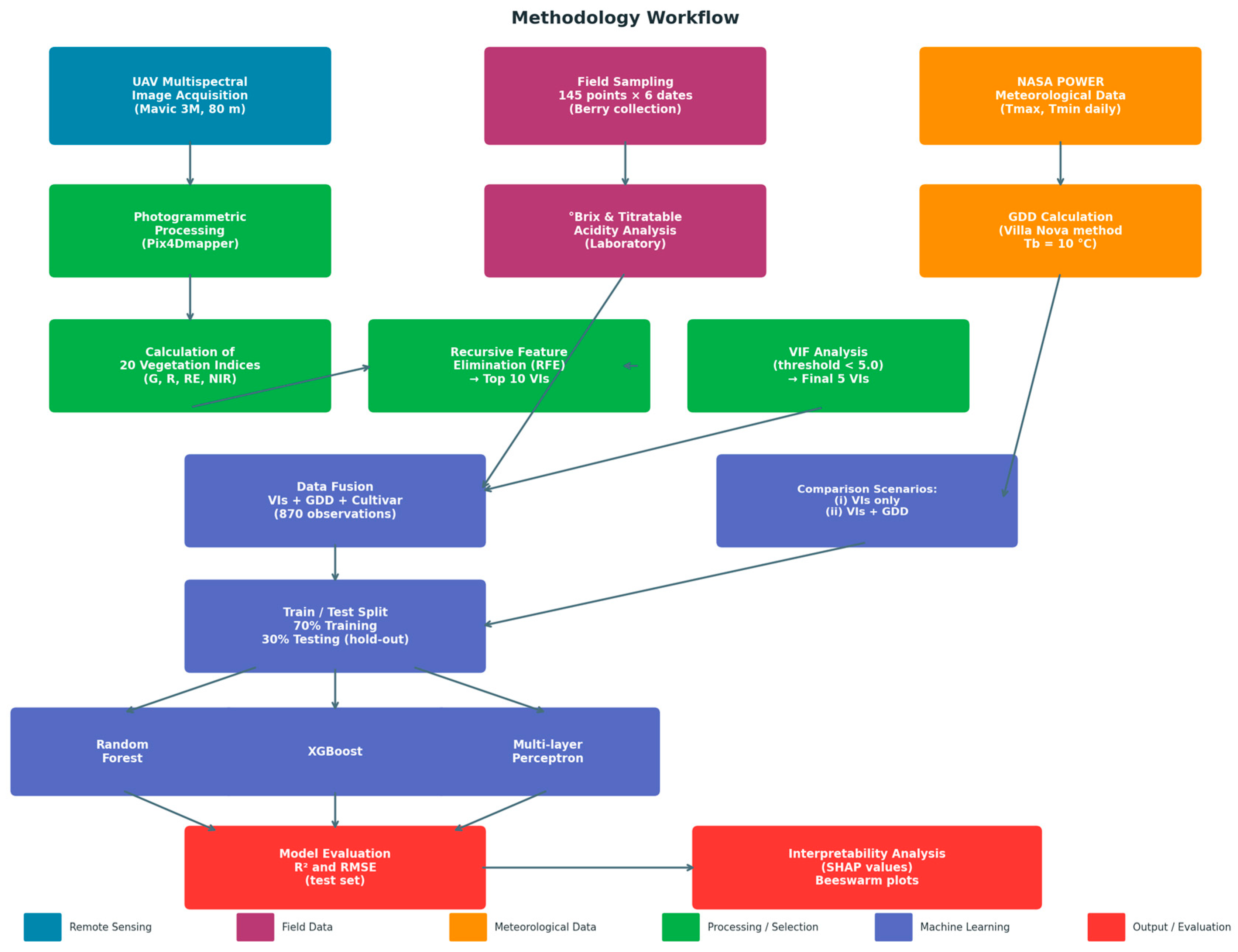
The analysis of SHAP values, visualized through beeswarm summary plots, allows for detailed interpretation. This type of plot displays the distribution of SHAP values for each sample and variable, ranking the variables by their global importance. Moreover, the plot uses color to represent the feature’s own value (high or low), making it possible to identify not only the magnitude of a predictor’s impact on the prediction but also its direction. This analysis, applied to the test set, was crucial for validating whether the relationships learned by the model are agronomically coherent and for building confidence in the results. The complete methodology workflow is summarized in Figure 2.

3. Results

3.1. Feature Selection Results

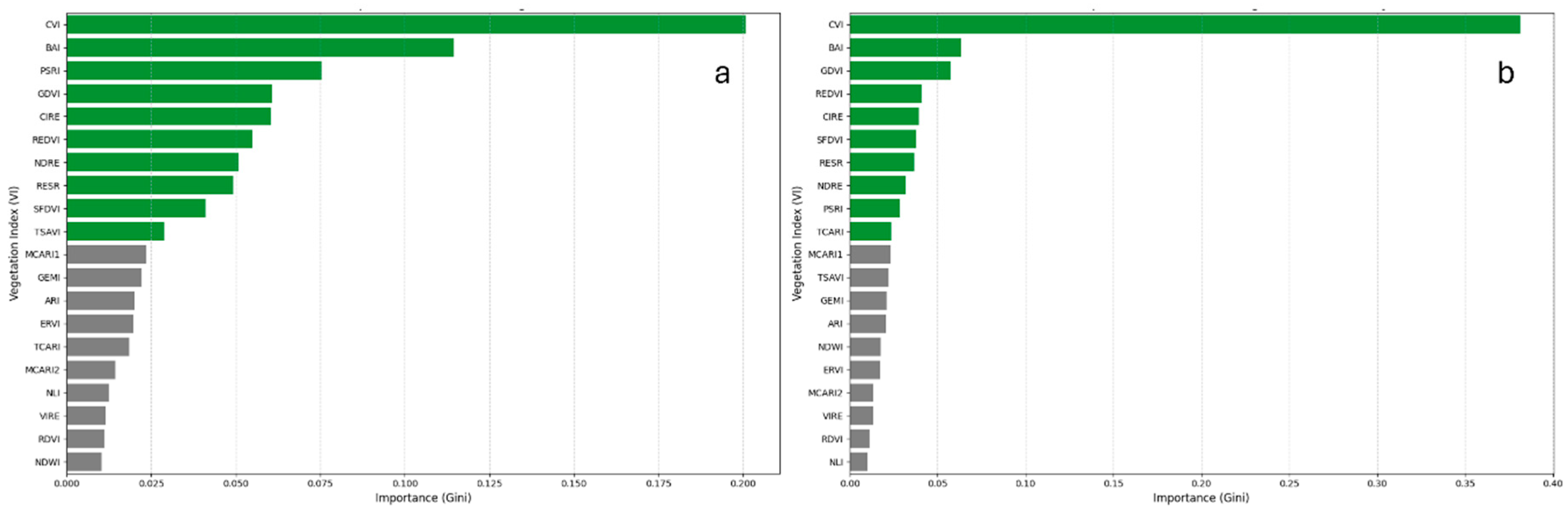
The first stage of the results consisted of filtering the 20 calculated Vegetation Indices (VIs), identifying the most relevant and independent subsets of predictors for modeling. The Recursive Feature Elimination (RFE) process ranked the 10 most promising VIs for each target variable, as detailed in Figure 3. Nine of these VIs were common to both targets (°Brix and Titratable Acidity): ‘CVI’, ‘BAI’, ‘PSRI’, ‘GDVI’, ‘CIRE’, ‘REDVI’, ‘NDRE’, ‘RESR’ and ‘SFDVI’. The distinctions in the RFE selection were the ‘TSAVI’ index (selected only for °Brix) and ‘TCARI’ (selected only for Titratable Acidity).

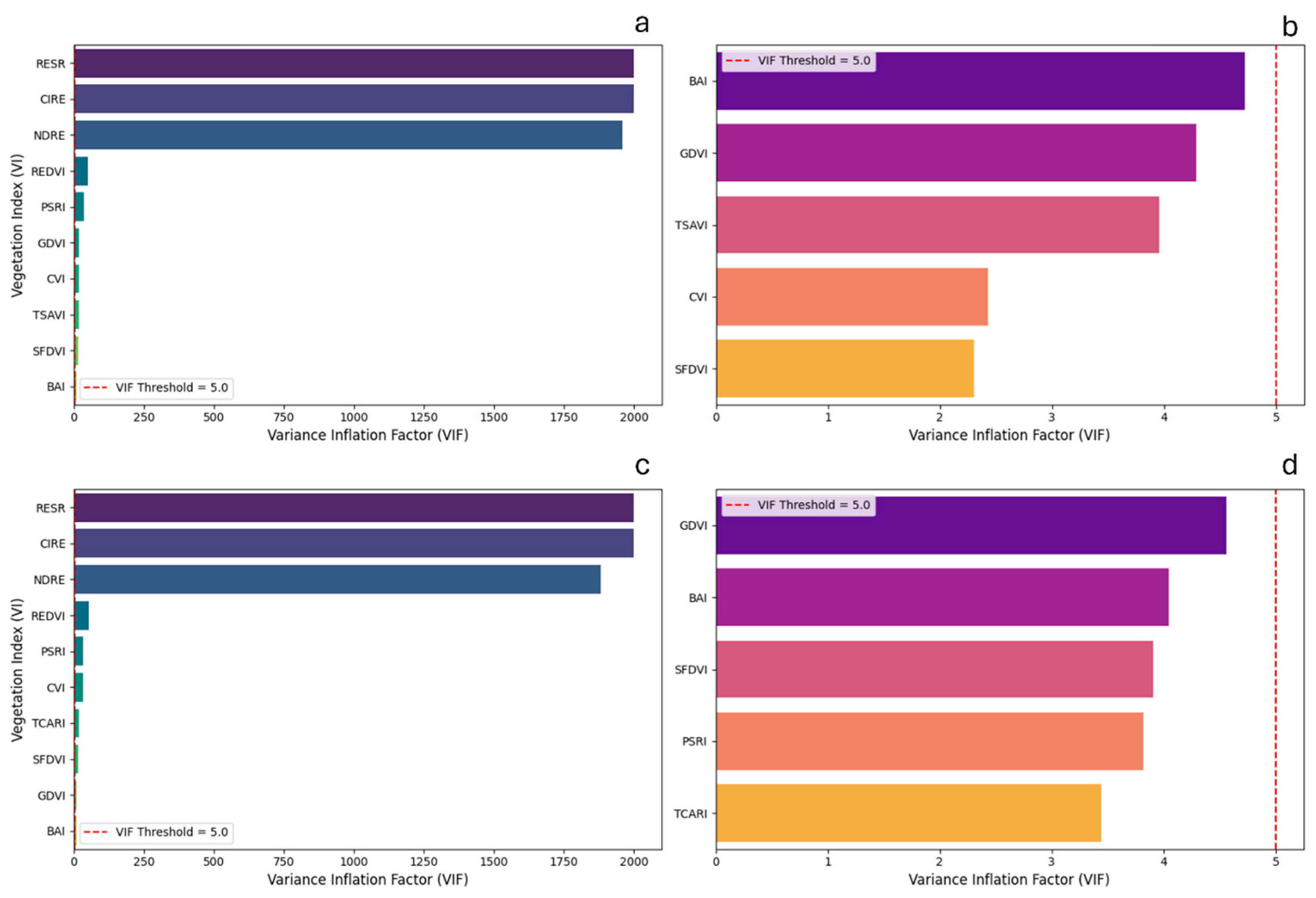
In the next stage, these two 10-VI sets were subjected to Variance Inflation Factor (VIF) analysis to mitigate multicollinearity. An iterative process was applied to remove the variable with the highest VIF until all remaining predictors had a VIF < 5.0. Figure 4 illustrates the iterative elimination process. The VIF analysis revealed extreme collinearity in both sets, notably in ‘RESR’ (VIF = ∞) and ‘NDRE’ (VIF > 1800 for both targets), indicating that their information was almost entirely redundant. For the °Brix model, the ‘PSRI’ (VIF = 37.05), ‘CIRE’ (VIF = 24.5), and ‘REDVI’ (VIF = 9.8) VIs were also removed. For the Titratable Acidity model, ‘CVI’ (VIF = 27.54), ‘CIRE’ (VIF = 24.9), and ‘REDVI’ (VIF = 9.71) were removed.

At the end of the selection pipeline, two final and distinct sets of five VIs were obtained: the set for °Brix was composed of ‘SFDVI’, ‘BAI’, ‘CVI’, ‘GDVI’, and ‘TSAVI’, while the set for Titratable Acidity included ‘SFDVI’, ‘BAI’, ‘GDVI’, ‘PSRI’ and ‘TCARI’. Three VIs (‘SFDVI’, ‘BAI’, ‘GDVI’) were selected as fundamental predictors for both variables. However, the models diverged in their specific predictors: ‘CVI’ and ‘TSAVI’ were uniquely selected for °Brix, while ‘PSRI’ and ‘TCARI’ were uniquely selected for Titratable Acidity. These two final, low-collinearity VI sets were then used for the modeling stage, both in isolation (IV-only models) and in fusion with the agrometeorological variable (GDD), to evaluate the impact of including the temporal predictor.

3.2. Predictive Model Performance for Technological Maturity

The performance of the machine learning models was evaluated in two distinct scenarios: (i) using only the selected VIs as predictor variables and (ii) with the fusion of these predictors with the temporal variable GDD. The results demonstrate the crucial impact of data fusion for the prediction of technological maturity.

Although the Random Forest model fit the training data better for °Brix prediction, none of the three algorithms was able to create a viable predictive model using only the VIs in the test stage. The drastic reduction in accuracy (R²) and increase in error (RMSE) between the training and test stages unequivocally demonstrate that these predictors, in isolation, do not provide sufficient information for the models to learn the relationship underlying technological maturity progression, leading them to memorize the specific noise of the training set instead of learning generalizable patterns.

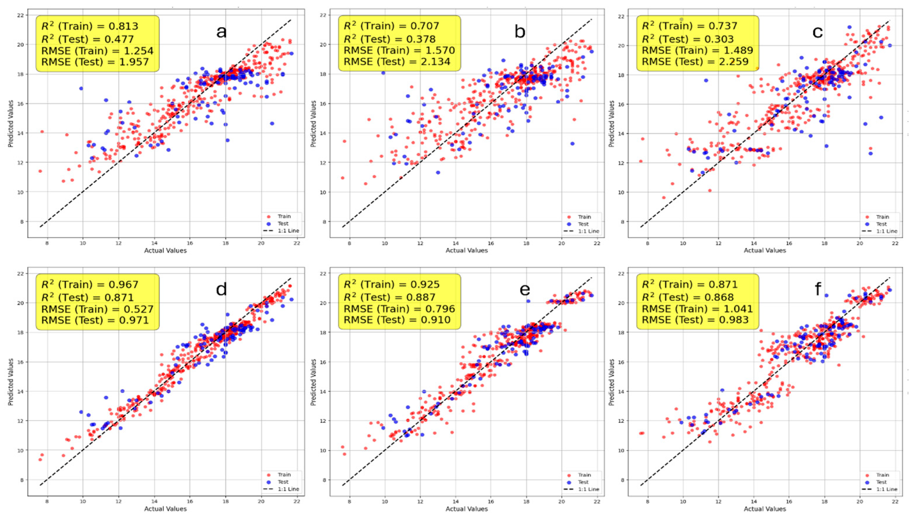
For °Brix prediction, although the coefficient of determination on the training set for the XGBoost algorithm was 0.707, the performance on the test set was drastically reduced, with an R² of 0.378 (Figure 5b). The behavior of Random Forest was similar. It showed a strong fit to the training data, with an R² of 0.813 and RMSE of 1.254. However, in the test stage, the performance was equally unsatisfactory, with the R² dropping to 0.477 and the RMSE increasing to 1.957 (Figure 5a). The MLP showed a similar fit to the XGB model on the training data (R² of 0.737); however, it registered the lowest performance on the test set (R² of 0.303 and RMSE of 2.259) among the models tested (Figure 5c).

Upon integrating the Growing Degree-Days (GDD) variable into the predictor set (Figure 5d–f), the performance of all models for °Brix estimation exhibited significant improvements in generalization capacity, especially regarding accuracy, with error (RMSE) values below 1 °Brix for all models.

To isolate the contribution of each data type, a third scenario was evaluated using only GDD and Cultivar as predictors (GDD-only). For °Brix prediction, the GDD-only XGBoost model achieved R² = 0.889 on the test set (RMSE = 0.99 °Brix), closely approaching the performance of the full VI + GDD model. For Titratable Acidity, the GDD-only model yielded R² = 0.844 (RMSE = 1.818 g/L). The date-index proxy analysis—substituting GDD with a simple ordinal temporal index (1–5)—produced R² = 0.815 for °Brix and R² = 0.821 for TA, compared to 0.84 and 0.806 for the GDD-based models (ΔR² = 0.025 and −0.015, respectively). These results indicate that the performance advantage of GDD over simple temporal ordering is marginal, particularly for TA prediction, and are discussed further in Section 4.

The XGBoost algorithm stood out with the best overall performance in predicting °Brix (Figure 5e). After being trained, it achieved an R² of 0.925 on the training set and, more importantly, maintained the most robust performance on the test set, with an R² of 0.887 and the lowest RMSE of 0.910. The Random Forest (RF) model showed a very competitive and close result (Figure 4d), with an R² of 0.967 on the training set and 0.871 on the test set, and an RMSE of 0.971. On the other hand, the MLP model (Figure 5f), which had shown inferior performance compared to the others in the previous scenario, also improved significantly when GDD values were added to the model, returning an error value (RMSE = 0.983) very close to that of the tree-based models. Furthermore, the MLP was the model with the lowest overfitting rate, with the training and test results showing a variation in only 0.003 in the coefficient of determination.

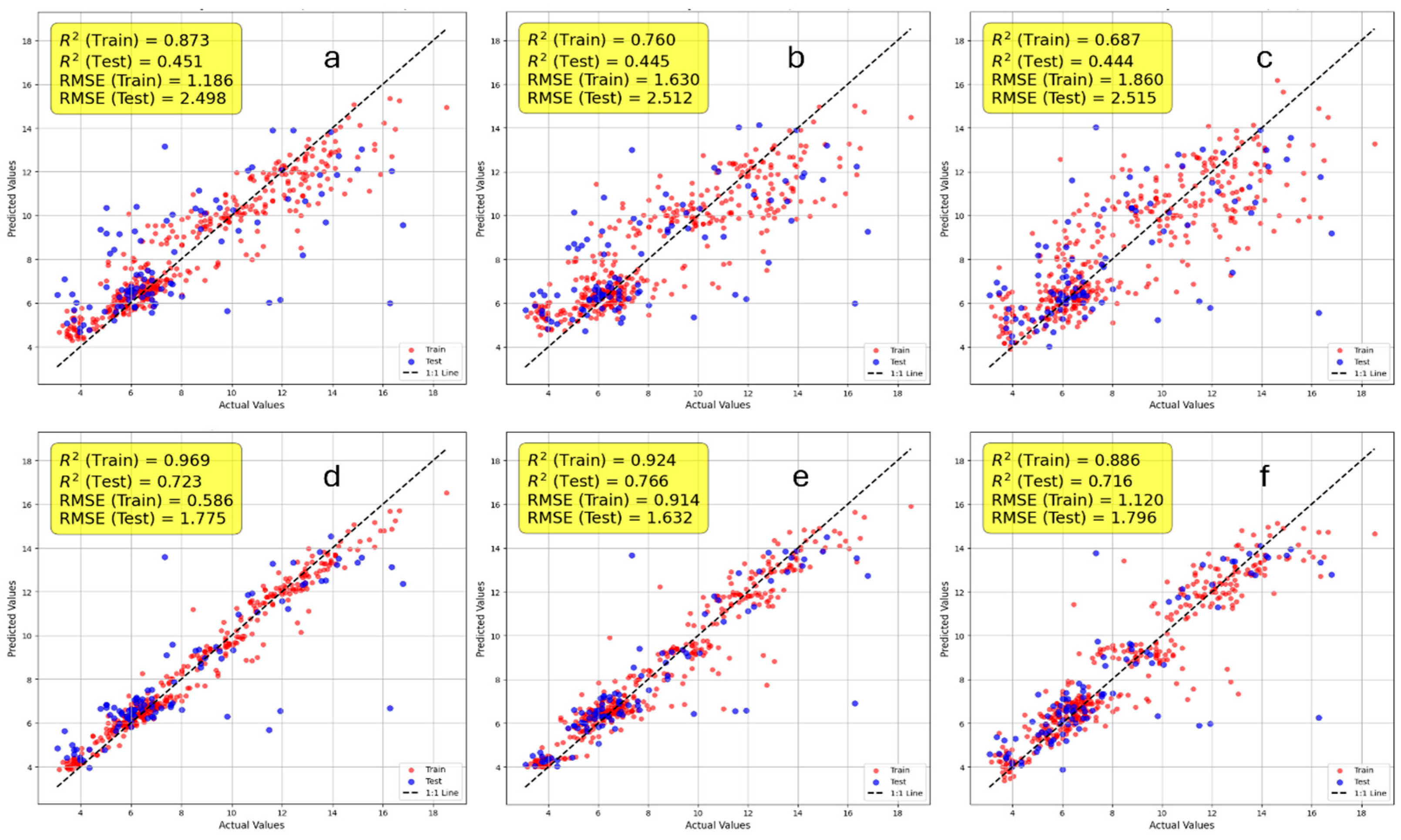
Similar to the performance found for °Brix prediction, the machine learning models that used only the VIs and ‘Cultivar’ as predictors did not produce generalizable estimates for Titratable Acidity (g/L). Although the tree-based algorithms fit the training data well (RF with R² = 0.873; XGBoost with R² = 0.760), their coefficients of determination on the test set were low, reaching only R² = 0.451 for RF and R² = 0.445 for XGBoost (Figure 6a,b). The MLP model showed the weakest fit on the training set (R² = 0.687) and the lowest performance on the test set (R² = 0.444) (Figure 6c). These results demonstrate the ineffectiveness of VIs alone for modeling the degradation of organic acids in grapes.

The inclusion of the GDD variable considerably improved the performance of all models. However, an overfitting trend persisted, with a reduction in accuracy (R²) observed between the training and test data. This drop was 25.4% for the Random Forest model (0.969 train vs. 0.723 test), 17.1% for XGBoost (0.924 vs. 0.766), and 19.2% for the MLP (0.886 vs. 0.716) (Figure 6d–f). Despite this, all models with GDD achieved test R² values greater than 0.70, which did not occur in any model without GDD.

Regarding the error (RMSE) in predicting Titratable Acidity in the GDD-inclusive scenario, the result achieved by the XGBoost model stood out by obtaining the lowest error in the test stage with 1.632 g/L. The other models showed slightly higher errors, at 1.775 g/L for Random Forest and 1.796 g/L for the MLP.

The comparative analysis demonstrates that, although all three algorithms became reasonable predictors after data fusion, XGBoost showed clear superiority, with the highest R² (0.766) and the lowest RMSE (1.632 g/L). This result validates the study’s central hypothesis regarding the importance of including climatic variables, but it also indicates that predicting Titratable Acidity is an inherently more complex task than predicting °Brix.

Statistical significance testing using the Wilcoxon signed-rank test on paired absolute residuals from the test set confirmed that XGBoost produced significantly lower errors than MLP for both °Brix (p < 0.001) and TA (p < 0.001). However, the error difference between XGBoost (R² = 0.867 for °Brix; R² = 0.833 for TA) and Random Forest (R² = 0.865 for °Brix; R² = 0.846 for TA) was not statistically significant (p = 0.4054 for °Brix; p = 0.5039 for TA), indicating that both tree-based ensemble approaches achieved equivalent predictive performance for this dataset. The best hyperparameters identified by the expanded XGBoost grid search were: learning_rate = 0.05, max_depth = 3, and n_estimators = 100 (for °Brix) and learning_rate = 0.05, max_depth = 3, and n_estimators = 100 (for TA).

3.3. Predictor Contribution Analysis (SHAP)

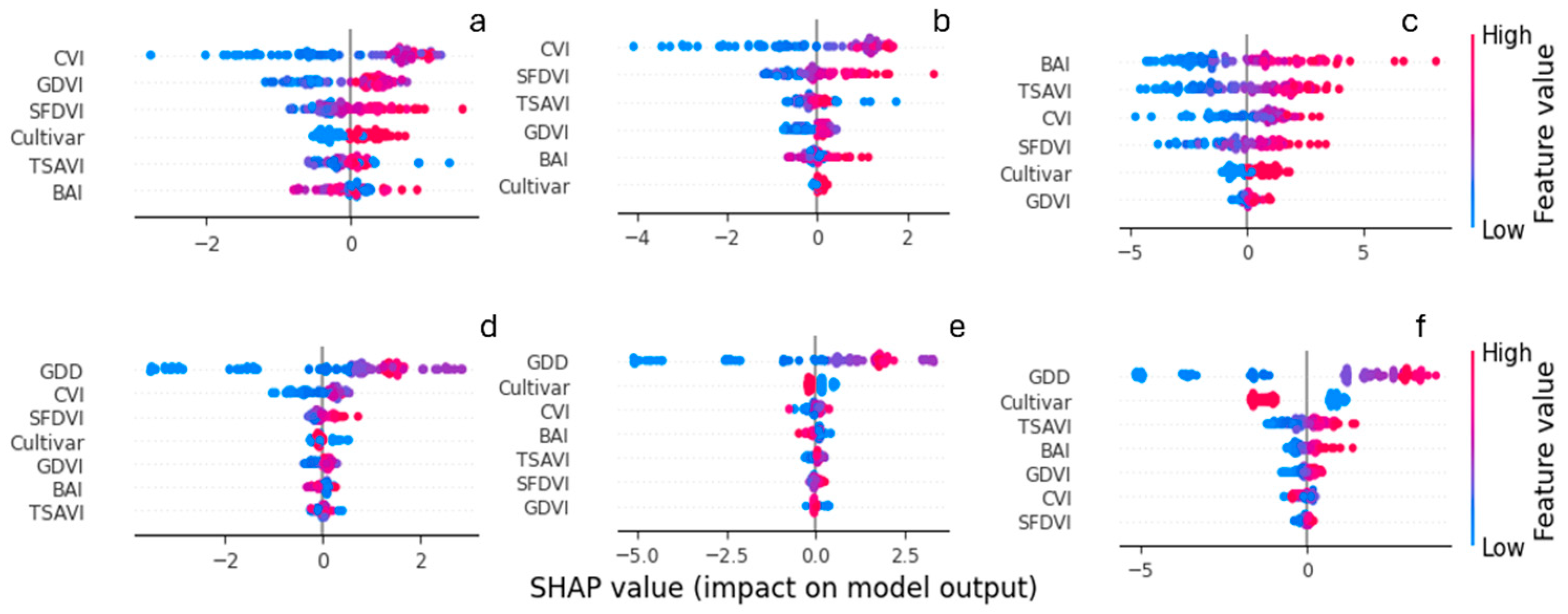
Interpretability analysis (SHAP) was applied to the °Brix models to understand each predictor’s contribution. In all data fusion models (Figure 7d–f), GDD was confirmed as the predictor with the highest global influence. The SHAP summary plot reveals an agronomically coherent relationship: high GDD values (indicating greater thermal accumulation) generate a positive impact, increasing the predicted °Brix value, which is consistent with the known phenological rule of ripening, in which thermal accumulation progressively drives sugar concentration in the berry.

A fundamental change was observed in the models’ internal behavior. In the GDD-absent (VI-only) scenarios, the tree-based models, Random Forest (Figure 7a) and XGBoost (Figure 7b), assigned the greatest weight to CVI. In contrast, the MLP (Figure 7c) prioritized BAI, although it distributed the importance more evenly among ‘BAI’, ‘TSAVI’, ‘CVI’, and ‘SFDVI’. This suggests that, in the absence of GDD, the models attempted to use proxies for vigor and chlorophyll content (like CVI) to estimate maturity.

However, with the inclusion of GDD, the feature importance hierarchy changed dramatically. As seen in the SHAP plots for all three models (Figure 7d–f), the ‘Cultivar’ variable consistently emerged as the second-most influential predictor, surpassing all Vegetation Indices. The detailed analysis (beeswarm plot) reveals how the generalist model functions: for a given GDD value, the model systematically assigns a higher impact (higher predicted °Brix) to one cultivar (represented in red) than the other (in blue). This demonstrates that the model did not create separate logics but instead learned a base relationship (Brix vs. GDD) that is then systematically adjusted according to the cultivar identity.

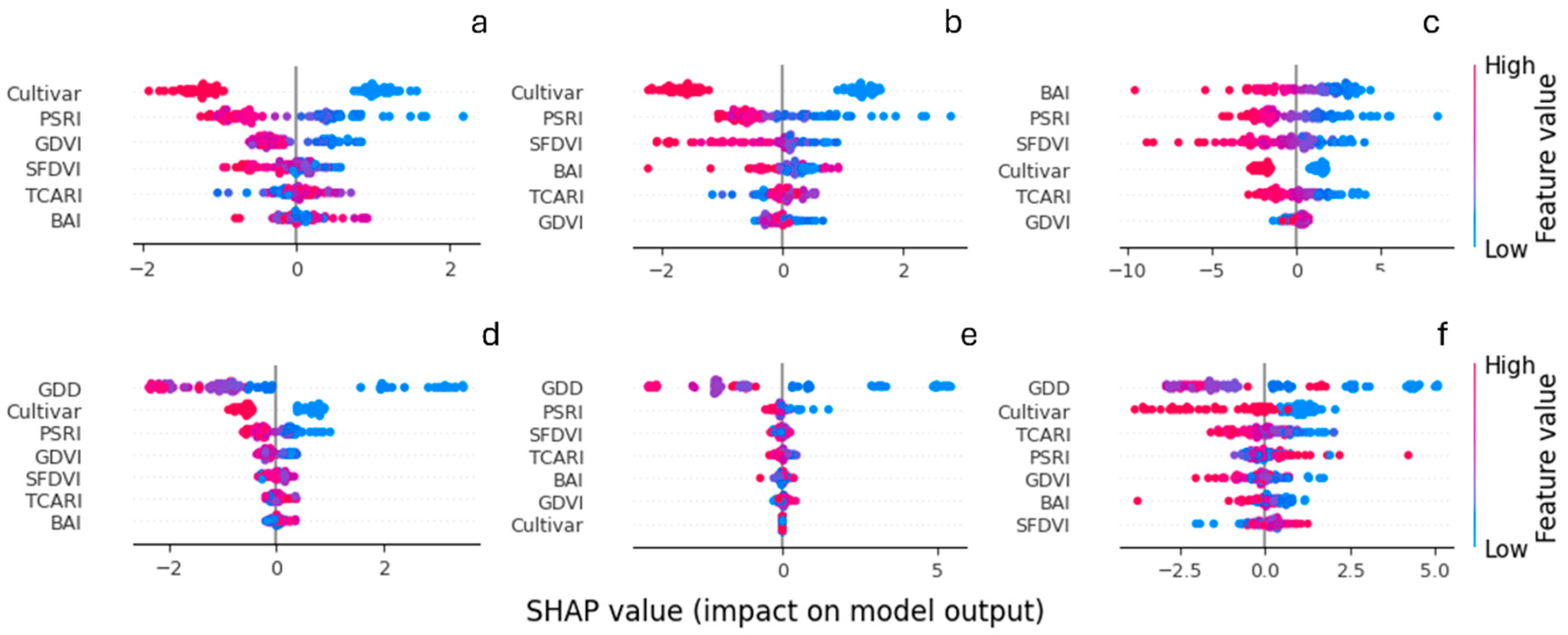
The SHAP analysis for the Titratable Acidity (TA) models reveals more complex behavior than that observed for °Brix (Figure 8). In the data fusion scenario (Figure 8d–f), GDD was consistently identified as the predictor with the highest impact across all three algorithms. As agronomically expected, the beeswarm plot demonstrates a strong inverse relationship: high GDD values (associated with advanced ripening stages) generate negative SHAP values, contributing to lower predicted acidity.

In the GDD-absent scenario, the models diverged. In the Random Forest (Figure 8a) and MLP (Figure 8c) models, the ‘Cultivar’ variable was the most influential factor, indicating that, lacking a temporal predictor, the grape’s genetic identity was the most important information for determining acidity levels.

The most significant change occurred in the importance hierarchy after GDD was included. In the Random Forest (Figure 8d) model, ‘Cultivar’ remained the second-most important variable, following GDD, demonstrating that the model captured both the temporal trend and the baseline genetic difference between varieties. The MLP (Figure 8f) also maintained ‘Cultivar’ as highly relevant, following its tendency for greater balance among predictors.

In striking contrast, in the XGBoost (Figure 8e) model, the inclusion of GDD caused the ‘Cultivar’ variable to drop to the last position in importance. The XGBoost model attributed almost all predictive power to GDD, with the VIs acting as secondary modulators. This fundamental difference in how XGBoost and Random Forest handled the ‘Cultivar’ variable is a crucial insight into the internal workings of the algorithms for this specific task.

Taken together, the SHAP interpretability analyses for °Brix and Titratable Acidity reinforce the relevance of the XGBoost model. It is evident that this model emerged not only as the most accurate predictor (R² = 0.887 for °Brix; R² = 0.766 for TA), but also as an interpretable model aligned with viticultural principles. The model demonstrated its ability to learn the opposing physiological dynamics (sugar accumulation and acid degradation) and to modulate both predictions based on cultivar identity. This approach validates the development of a single, generalist, and physiologically aware model for estimating technological maturity.

From a physicochemical perspective, the predominance of GDD across all models reflects its role as the primary integrator of veraison-associated metabolic processes. During grape ripening, sucrose imported from photosynthetically active leaves is hydrolysed by invertase into glucose and fructose, with this enzymatic activity being thermally regulated and tightly coupled to accumulated heat units [30]. The second-order importance of ‘Cultivar’ in the SHAP hierarchy is consistent with the distinct metabolic profiles of Sauvignon Blanc and Syrah, which differ substantially in the activity of malic enzyme and malate dehydrogenase—enzymes governing the rate of malate degradation and, consequently, the trajectory of Titratable Acidity decline during ripening [30]. The VIs, functioning as tertiary predictors, capture within-cultivar spatial heterogeneity in canopy photosynthetic capacity and chlorophyll content, which modulates the source–sink balance and thereby the rate at which individual vines deviate from the cultivar–GDD maturation trajectory. These patterns are consistent with known grapevine physiology; however, as SHAP values reflect model-internal associations rather than causal pathways, these interpretations should be regarded as hypothesis-generating rather than mechanistically conclusive.

4. Discussion

The central finding of this study is the unequivocal demonstration that Vegetation Indices (VIs) alone are insufficient predictors of grapevine technological maturity. Our results showed that, despite a rigorous feature selection process, the VI-only models failed to generalize, exhibiting low R² (0.30–0.47 for °Brix) and high overfitting. This finding corroborates the results of [8,9], who, despite testing different sensors and algorithms, also reported modest R² values (0.52 and 0.61, respectively). This reinforces our initial hypothesis: VIs provide a spatial “snapshot” of canopy vigor but lack the crucial temporal dimension that governs phenology. The inclusion of Growing Degree-Days (GDD) as a temporal predictor resolved this gap, transforming non-viable models into high-precision tools (R² > 0.88 for °Brix with XGBoost). GDD acted as the model’s “backbone,” providing the baseline trajectory of physiological development (sugar accumulation and acid degradation), while the VIs and the ‘Cultivar’ variable acted as secondary modulators, refining the prediction based on spatial vigor variability and genetics.

Regarding the analyses for selecting model inputs, collinearity among VIs is often overlooked, and models are generated with numerous VIs as predictors [9,31,32,33]. In most cases, only a relevance-focused feature selection (like RFE) is applied, without redundancy analysis. Many VIs are mathematical derivations that use the same spectral bands, resulting in informational redundancy. The application of a strict statistical criterion, such as a VIF threshold of 5.0 [34,35], was a crucial methodological step to mitigate this redundancy, ensuring the robustness and interpretability of the final model, following established recommendations for handling collinearity in multivariate explanatory models [36,37].

The result of this filtering was the non-selection of established indices like NDVI. VIs such as NDVI, NDRE, and GNDVI are widely used for predicting biomass and yield [5]. However, our results indicated that other VIs, such as CVI, SFDVI, and BAI, contributed more to predicting maturity. Although NDVI is an excellent indicator of general vigor, we suggest that its known saturation in dense canopies, such as grapevines, limited its ability to identify the subtle phenological changes associated with fruit ripening. This saturation phenomenon is well documented for vegetation canopies with a Leaf Area Index (LAI) exceeding approximately 3.0, beyond which NDVI asymptotically plateaus at values above 0.80 regardless of further increases in biomass or chlorophyll content [5,6]. Although a formal analysis of per-date reflectance distributions for this specific vineyard is deferred to the next revision stage, consistently elevated NDVI values throughout the ripening period are consistent with the known saturation behavior of this index in commercially managed, high-density grapevine canopies. This does not invalidate NDVI, which is indeed effective for yield prediction [38,39]. However, to estimate grape quality, the literature has already reported that it should be used in association with other data, which reinforces our data fusion approach [40,41].

Similarly, NDRE, which uses the red-edge band for a better estimate of chlorophyll content, was pre-selected by RFE. However, its subsequent removal due to an extremely high VIF (VIF > 1950) indicates that its information was already contained in other predictors, such as CVI and REDVI, which proved to be more relevant and less redundant. This reinforces that the choice of the best spectral predictors is highly dependent on the agronomic target and that a data-driven approach, such as the one we used (RFE + VIF), is superior to the simple adoption of conventional indices. It should also be acknowledged that the feature selection pipeline employed Random Forest as the base estimator for RFE, which may introduce a selection bias towards features that are particularly informative for tree-based ensemble methods, potentially yielding suboptimal feature subsets for XGBoost and MLP. Algorithm-specific or multi-learner feature selection strategies could be explored in future work to address this limitation.

Even after applying variable selection criteria and using only those of a spectral nature that contribute to predicting grape technological maturity, it is worth highlighting, among our study’s main results, the low accuracy of machine learning models in predicting this maturity when VIs are used exclusively as input data. This result should be considered a point of caution for most growers, especially given the growth of service providers using drones for mapping linked to grapevine quality and justifying the use of these data as support for field decision-making. Thus, as demonstrated, regardless of the algorithm’s architecture, the resulting models exhibited overfitting, combining good performance on the training data with insignificant predictive performance on the test set.

This low accuracy stems from a conceptual limitation wherein VIs provide spatial information on the canopy’s physiological state but lack the temporal dimension that governs the ripening process. Ripening is a cumulative process, intrinsically linked to accumulated thermal energy (GDD) throughout the phenological cycle [42,43]. A vine can exhibit the same vigor, and therefore have the same VI value, at different developmental stages but with completely different fruit compositions. Without the temporal context provided by GDD, the models were unable to resolve this ambiguity, resulting in models with training R² values up to 0.81 (for RF), but with test R² values falling as low as 0.30 (for MLP) and never exceeding 0.48. Despite the low values found in our work using only VIs as input, [9] also reported low accuracy values when they tested different sensors to predict grape quality attributes.

The inclusion of GDD improved the performance of the models, especially in the test stage, validating the central hypothesis that data fusion is essential. The SHAP interpretability analysis was fundamental for decoding the internal workings of the final XGBoost model, revealing how this synergy operates and confirming that the model learned to replicate the physiological logic.

The interpretability analysis (SHAP) consistently revealed, across the three tested models, that GDD was the predictor with the greatest impact and potentiated the prediction of grape development, as also observed for other crops [11,12,44]. This result corroborates field observations, as GDD functions as a direct indicator of the grapevine’s phenological development stage [45,46].

The SHAP results suggest a clear hierarchy: GDD and ‘Cultivar’ establish the baseline prediction, defining the expected maturity potential for that cycle stage and genetic variety. The VIs, in turn, act as secondary predictors. They modulate the baseline prediction by capturing spatial variability in the crop’s physiological conditions, such as localized stresses or vigor differences, which cause a plant to deviate from the general trend expected for its GDD and cultivar. Furthermore, the importance of ‘Cultivar’ in the SHAP analysis demonstrates the model’s ability to learn and quantify the genetically distinct ripening profiles between Sauvignon Blanc and Syrah, a fact aligned with physiological knowledge about sugar accumulation and acid degradation in different varieties [30].

However, an important methodological caveat applies to the interpretation of ‘Cultivar’ importance in the SHAP analyses: the two cultivars occupy spatially distinct blocks with different row orientations (Sauvignon Blanc: NE-SW; Syrah: NW-SE), meaning that ‘Cultivar’ is inherently confounded with block-level spatial factors, including canopy geometry, differential solar irradiance exposure, and localized microclimate variability. Consequently, the SHAP-attributed importance of ‘Cultivar’ reflects an undifferentiated composite of genetic ripening dynamics and spatial-environmental co-factors, and it is not possible within the current experimental design to attribute this contribution exclusively to genotypic differences in metabolic processes. Future studies should consider implementing cultivar-specific sub-models or incorporating spatial covariates such as topographic aspect and slope to disentangle these confounded effects.

However, the way this genetic influence interacts with remote sensing signals can be modulated by management factors, leading to sometimes divergent results in the literature. For instance, we observed that, under irrigation, VIs were less effective in predicting quality for Sauvignon Blanc compared to Syrah, demonstrating a complex interaction between cultivar and water management [47]. Conversely, the work by Santos [48] found robust correlations in Vitis vinifera L., suggesting the potential of VIs to replace conventional analyses in certain contexts. This apparent inconsistency in the literature does not invalidate the results presented here; on the contrary, it demonstrates that Vitis vinifera L. is extremely sensitive to local interactions among genotype, environment, and management. Therefore, the calibration of generalist models, as performed in the present study, is an indispensable step for the successful application of remote sensing tools in decision-making.

Among the evaluated models, XGBoost showed the highest accuracy, a result frequently observed in agricultural applications due to its efficiency in handling tabular data and complex non-linear relationships [49]. It is important to note, however, that all models (including RF and MLP) achieved high performance after the inclusion of GDD, suggesting that the quality of the predictor variables was more decisive than the choice of the specific algorithm.

Several methodological and contextual limitations of this study warrant explicit discussion. First, the dataset encompasses a single growing season (2024) at one commercial vineyard, constraining generalizability to season-specific climatic patterns and the particular agronomic conditions of this site. Second, GDD was accumulated over only six discrete collection events, making it nearly co-linear with the temporal ordering of sampling; a date-as-surrogate sensitivity analysis was performed: replacing GDD with an ordinal temporal index (1–5) yielded R² = 0.815 (°Brix) and R² = 0.821 (TA), compared to 0.84 and 0.806 with GDD (ΔR² = 0.025 and −0.015). For TA, the date proxy marginally outperformed GDD, indicating that temporal ordering rather than thermodynamic accumulation may drive a portion of the predictive signal in this five-date dataset. Third, the stratified hold-out split did not account for spatial autocorrelation among the 145 georeferenced points across collection dates; a GroupKFold analysis stratified by point identity is planned. Fourth, the ‘Cultivar’ predictor is spatially confounded with block geometry and microclimate, limiting mechanistic interpretation of its SHAP-ranked importance. Fifth, the RFE pipeline employed Random Forest as the base estimator, potentially yielding suboptimal feature subsets for non-tree-based algorithms. Sixth, SHAP values reflect model-internal association patterns and do not establish causal relationships. Finally, soil properties, vine water status, and thermal heterogeneity within the vineyard were not incorporated as predictors, representing avenues for model improvement in future multi-sensor, multi-season studies.

5. Conclusions

The fusion of remote sensing data (Vegetation Indices) with the temporal variable Growing Degree-Days (GDD) proved to be a fundamental and highly effective approach for predicting Soluble Solids (°Brix) and Titratable Acidity in wine grapes grown under a double pruning system. The study validated its central hypothesis by demonstrating that the inclusion of GDD significantly improved accuracy, transforming models based only on VIs, which were shown to be incapable of generalization (test R² < 0.48), into robust prediction tools.

Furthermore, the most influential and least redundant VIs for prediction were identified, such as ‘CVI’, ‘SFDVI’, and ‘BAI’, whereas traditional indices (‘NDVI’ and ‘NDRE’) which were removed due to saturation or high multicollinearity. Among the evaluated algorithms, XGBoost was determined to have the best predictive performance for both target variables, achieving a test set R² of 0.89 for °Brix and 0.77 for Titratable Acidity.

This work therefore reinforces that the fusion of temporal (GDD) and spatial (VI) data is a prerequisite for the accurate modeling of grapevine technological maturity. These findings constitute a promising proof-of-concept for non-destructive maturity prediction in precision viticulture; however, validation across multiple growing seasons and vineyard environments is essential to confirm the broader applicability and operational reliability of the proposed framework.