Article

Trends in Global Grape Production over Six Decades: Leading Countries, Market Concentration, and Future Projections Based on ARIMA Modeling


1
Department of Horticulture, Faculty of Agriculture, Atatürk University, Erzurum 25240, Türkiye
2
Department of Agricultural Economics, Faculty of Agriculture, Atatürk University, Erzurum 25240, Türkiye
*
Author to whom correspondence should be addressed.
Horticulturae 2026, 12(6), 658; https://doi.org/10.3390/horticulturae12060658
Submission received: 11 March 2026 / Revised: 21 May 2026 / Accepted: 22 May 2026 / Published: 24 May 2026

Abstract

Viticulture is a globally significant economic activity; however, the scientific literature lacks in-depth, long-term studies integrating historical trends with future market concentration projections. This study fills this gap by analyzing global grape production dynamics and market structure over a 63-year period (1961–2023). The detection of structural breaks and the forecasting of yield trajectories using AutoRegressive Integrated Moving Average with Exogenous Variables (ARIMAX) models are crucial for the strategic planning of agricultural resources and enhancing viticultural resilience. Results indicate that while the global population increased 2.58-fold (1961–2023), grape production rose only 1.69-fold, leading to a decline in per capita availability. Although traditional leaders remain dominant, the combined share of the top five producers fell from 60% to 51.8%. The market concentration analysis Herfindahl-Hirschman Index (HHI) = 0.092; the Concentration Ratio (CR5) = 53.65%) for 2024–2030 suggests a monopolistic competition structure. The arithmetic mean of annual global production for the 2024–2030 period is projected to reach 79.42 million tons. China is expected to lead (23.11%), followed by Italy, the United States, France, and Spain. These findings highlight the necessity of precision viticulture and modern technology to stabilize yields and enhance competitiveness in high-value horticultural markets.

1. Introduction

Agricultural production plays an important role in the determination of global economic and socio-cultural processes. Viticulture is of strategic importance for global food security, sustainable agricultural policies, and rural development. It is a large-scale activity in different climatic regions worldwide [1,2]. Grapes are a multibillion-dollar global industry with several end uses that increase their economic value, such as fresh consumption, drying, winemaking, and industrial processing [3,4]. However, while the global population has increased exponentially, grape production has not increased proportionally, which resulted in a decline in per capita production and consumption emphasizing an imbalance in global production and distribution systems.
Historically, a few countries have dominated grape production; European countries (notably Italy, France, and Spain) account for a large share of global production, while Türkiye accounts for about 5% of the total [5]. Complex interactions of genetics (G), environment (E), and management (M) control worldwide viticultural dynamics. Understanding this Genotype X Environment (G X E) interaction [6] is essential to evaluate the behavior of various types of vines and rootstocks in ecological contexts, especially in terms of the stability of production and quality preservation. In addition, climate change presents a redistribution of traditional viticulture regions and the increased risk of novel pests and diseases due to increased temperatures, unpredictable precipitation patterns and extreme weather events [7,8,9,10]. Such environmental perturbations have a direct impact on vine physiology and change important phenological events such as budburst, flowering and ripening [7]. Such phenological changes affect, in turn, secondary metabolites, final product quality and sugar–acid balance [8]. Modern agronomic practices are needed to solve these problems for long-term sustainability. The implementation of smart farming technologies, precision irrigation and biotechnological methods can improve production efficiency and reduce climate risks and the competitiveness of viticulture at the global level [11,12].
Since the 1960s, the mainstays of world grape production have been Italy, Spain, and France. But the emergence of the United States in the 1970s and China in the 2000s has structurally altered this competitive landscape, mirroring larger regulatory and institutional changes in both traditional and emerging wine-producing regions [13]. These geopolitical expansions are unfolding in the context of mounting climatic stresses that jeopardize the geographic viability of traditional European vineyards [14]. The five biggest grape-producing countries took about 60% of the world market share in the 1960s, 53% in the 1990s, and 51.9% in the 2010s (data from FAOSTAT [15]), with a relative stability at 51.8% projected at the end of the 2020s. In Europe, traditional leaders still have strong sectoral bases [16,17], but a new wave of agricultural investment and changing trade patterns has led to new competitive producers across Asia, South America, and Africa [18].
The global distribution and development of grape production provide a valuable perspective on the structure of the global market. Although the total share of major growers in the world production has been declining, the analyses based on the Herfindahl-Hirschman Index (HHI) [19] show a gradual shift in the world grape market from a competitive to a more oligopolistic market structure over time. These developments will alter not only the global pattern of production but also international trade networks and market mechanisms. They underline the need for producing countries to strengthen their position in the export markets for high-quality grapes and grape-derived products. In the past few decades, the world trade in vine growing and grape products has become more competitive than before. This has created new opportunities and challenges for producing countries and the global agricultural economy [18].
Continuous empirical monitoring of grape production and marketing is necessary to guide targeted agricultural policies and support programs as a dynamic horticultural sub-sector. The policy frameworks should simultaneously enhance the climate resilience of the growers and increase productivity under increasing environmental pressures. Moreover, the grape industry must adapt to changing market trends and consumer preferences, which are increasingly shaped by health and environmental considerations, as evidenced by the rising demand for organic and locally sourced grapes, to ensure long-term sustainability [20]. Therefore, sustainable practices, technical support, and technological innovations are key strategic imperatives for increasing the competitiveness of the sector and for securing the international market position of the producing nations.
Recently, the rapid development of the international viticultural literature has been driven by the integration of advanced forecasting technologies. From a methodological perspective, predictive frameworks have evolved from the comparison between conventional econometric tools, such as AutoRegressive Integrated Moving Average (ARIMA) and Exponential Triple Smoothing (ETS) models, in different orchard systems and vineyards [21,22], to the use of machine learning algorithms combining soil and meteorological datasets for dynamic yield optimization [23,24]. Moreover, there is an evident paradigm shift from baseline volume projections to product quality, price volatility, and climate-driven sectoral sustainability [25,26]. Recent studies have employed sophisticated machine learning architectures, GARCH variants, and BiLSTM neural networks to model wine quality, market values, and macroeconomic fluctuations [27,28,29]. Since forecasting errors can result in huge financial losses in the supply chain, it is essential to develop highly reliable and low-deviation modeling configurations to minimize the direct effects of annual weather anomalies on regional and global productivity [30,31,32].
Although previous studies have demonstrated progress, a key research gap still exists. Prior literature has largely focused on localized, short-term yield estimations without linking long-run production macrotrends and shifting global market power configurations. This study fills this gap by integrating a large 63-year longitudinal dataset (1961–2023) to produce reliable short- and medium-term global production forecasts. Methodologically, this study differs from traditional research focused solely on estimation, as it uniquely combines projections with the HHI and CR5 to assess the ongoing oligopolization of the global market. Thus, the main goal of this research is to explain the direct link between technological or climate-related risks and the changing competitive landscape of the global viticulture industry from an integrative macro-level perspective.
Research questions
To guide this study, the following research questions were formulated, directly linking them to the methodology employed:
What are the long-term trends in global grape production from 1961 to 2023?
  • How have the production dynamics of major grape-producing countries evolved over time?
  • What structural changes have occurred in the global viticulture sector, and how can they be quantified?
  • How is market concentration in the global grape industry distributed, and how does it evolve according to the HHI and CR5?
  • How accurately can the ARIMA model forecast short- and medium-term grape production trends for leading countries?
  • What insights can be drawn to support sustainable production strategies and enhance competitiveness in the global grape market?

2. Materials and Methods

2.1. Materials

This research utilizes quantitative data about grape production at national and global scales. The main data sources are official statistics from the Food and Agriculture Organization of the United Nations (FAO) Statistical Database (FAOSTAT). In accordance with FAOSTAT and international reporting standards, production data represent total grape production, including table grapes, wine grapes, and grapes intended for drying (raisins). A comprehensive data preprocessing step was performed to ensure the robustness of the time series analysis. This rigorous validation process ensured that the dataset met the linear and exogenous requirements of the ARIMA and ARIMAX modeling applied in this study. Alongside these primary materials, secondary resources like academic theses, research reports, scholarly books, and peer-reviewed journal articles were used. This study of worldwide and national long-term production dynamics has been performed using a comprehensive dataset during 1961–2023, including annual volumes of grape production, harvested areas, yield rates, and shares in production of the top producer countries. The historical dataset was used only for training the model and estimation of the parameters, and afterwards, production forecasts were generated for the 2024–2030 period. To rigorously test the real-world predictive performance of the selected models, we designated the year 2024 as an external (out-of-sample) validation year. Consequently, the actual 2024 production data recently released by the FAO was excluded from the model training phase and used exclusively to assess and validate the accuracy of the models’ 2024 forecast values.
The ten leading countries (China, Italy, France, Spain, USA, Türkiye, India, Chile, South Africa, and Argentina) were selected on the basis of their contribution to the world production to ensure the statistical validity of the study. These countries together represent approximately 70% of total production, ensuring that the study captures the main trends in the global viticulture sector and provides a sound basis for international comparison.

2.2. Methods

The analysis of the data collected for this study was conducted using the Statistical Analysis System (SAS) version 9.4. Time series analysis was performed to examine temporal variations and to generate forward-looking forecasts using the econometric method known as ARIMA. This approach allows for statistically valid and reliable forecasting scenarios by taking into account the structural characteristics of time series data. Additionally, Microsoft Excel was employed as an auxiliary tool for graphical presentation and visual interpretation of the forecasted values.

2.2.1. Box–Jenkins (ARIMA) Forecasting Method

Methodological Rationale and the ARIMA Framework
Non-stationary structures in time series often exhibit pronounced stochastic behavior, making direct analysis and forecasting challenging. To address this issue, Box and Jenkins developed a stochastic theory-based time series modeling framework in 1970, which provides an effective analytical approach for non-stationary series [33]. The fundamental models within this framework include Autoregressive (AR), Moving Average (MA), and ARIMA models.
The construction of an ARIMA(p,d,q) model consists of four main steps. The first step involves determining whether the series is stationary, which is a prerequisite for time series modeling. In cases where the series is non-stationary, differencing of order 1, 2, or 3 is applied to stabilize its statistical properties over time. In the second step, the key parameters of the model, autoregressive order (p), differencing degree (d), and moving average component (q), are identified [34]. During this process, unit root tests are generally used to assess stationarity, while Autocorrelation Function (ACF) and Partial Autocorrelation Function (PACF) graphs contribute to the specification of model structure [35].
The third step was to check the statistical significance of the estimated parameters and the model’s explanatory power by applying rigorous residual diagnostics to verify whether the residuals follow the white noise properties. In addition to visual inspection, series stationarity was formally tested using the Augmented Dickey–Fuller (ADF) unit root test. The optimal values of model parameters (p,d,q) were determined by a structured decision framework: d was decided by ADF tests, and the initial candidate models were chosen by Smallest Canonical Correlation (SCAN) and Extended Sample Autocorrelation Function (ESACF) methods. Model configuration was selected based on the lowest Akaike Information Criterion (AIC) and Bayesian Information Criterion (BIC) values to achieve a parsimonious fit [36]. The out-of-sample forecasting performance was assessed by comparing the 2017–2023 forecasts to the actual observations using the Mean Percentage Error (MPE). Importantly, the ARIMAX framework was applied a priori with exogenous dummy variables; this systematic process was used for baseline stochastic paths with high MPE values resulting from documented extreme weather disruptions, capturing non-linear shocks that cannot be theoretically accommodated with univariate ARIMA models over sixty-year global agricultural cycles.
The final step involves evaluating the model’s overall fit and forecasting performance on the dataset to confirm its validity. In this regard, the ability of the ARIMA model to represent historical data and its predictive accuracy for future values are validated through multiple performance criteria.
The model that yielded the best results based on these criteria was selected as the optimal model [37,38].
y t = ( α + i = 1 p φ i y t i + ε t )   and
α = µ ( 1 φ 1 φ 2 φ P )
The MA model is as in Formula (3).
y t = ( α + i = 1 q θ i ε t i )
The ARMA model is expressed as in Formula (4).
y t = ( α + i = 1 p φ i y t i + ε t ) + ( i = 1 q θ i ε t i )
For the ARIMA model, we apply differencing to the ARMA model. Rather than showing multiple equivalent forms, we present the standard ARIMA(p,d,q) representation in Formula (5) [39,40].
φ B 1 B d y t = θ B ε t
The standard ARIMA structure can be extended to include exogenous variables in ARIMAX models, which provides a multidimensional causality insight in time-series analysis [41] by combining both historical lags and external structural shocks. For this study, one to seven exogenous dummy variables (X1, X2, …, X7) were included to capture country-specific economic or structural dynamics and to optimize forecasting performance. The decision for standard ARIMA or ARIMAX was solely based on the occurrence of statistically significant structural breaks or volatility in the data of each country. The stable series was modeled using the baseline ARIMA, while the anomalous series was modeled via ARIMAX. The exogenous interventions are coded as binary indicators (1 for shock years, 0 otherwise), matching the identified historical production anomalies. The biological and climate rationales for such interventions include extreme weather shocks such as the catastrophic late spring frosts in France (1991, 1992), the multiyear drought cycles in Spain culminating in 2023, and unseasonal monsoonal rainfall failures in India (where X1 and X2 explicitly captured structural shocks in 2012 and 2023, respectively). Table 3 lists country-specific variables and the precise timing of the shocks. The mathematical specification of the ARIMAX(p,d,q) formulation is presented in Equation (6).
φ P B 1 B d Y t =   θ q B ε t + β 1 X 1 + β 2 X 2 + + β 7 X 7
  • The symbols in the above formulas are expressed as follows:
  • d: Degree of differencing,
  • (1 − B)d = denotes the dth order difference operator,
  • Yt = t has tracked the observation values in the time series,
  • α = fixed number,
  • φ i = i change the parameters of yt−i at latency,
  • εt = white noise at time t shown as (WN(0, σ2)),
  • p = maximum latency time for AR,
  • q = maximum latency time for MA and,
  • θ i = i indicate the parameters of the εt−i at the latency.
The 1962–2030 period corresponds to the 95% confidence intervals (prediction limits). These limits represent the statistical variance for both the in-sample historical fit and the out-of-sample projections, providing a measure of the model’s precision throughout the entire analysis timeline.
Justification of Forecasting Approach: ARIMA Methodology vs. Alternative Models
In this study, ARIMA-based forecasting is performed on the principle of parsimony formalized by Box and Jenkins [42]. The principle states that the model should explain as much as possible with as few parameters as possible to reduce the risk of overfitting, especially for annual datasets with limited observations. Compared with Exponential Smoothing (ETS) models that mainly decompose independent trend and seasonality components, ARIMA architectures provide more flexibility in modeling non-stationary stochastic dependencies through internal autocorrelation mechanisms [43]. In addition, an emerging literature demonstrates that traditional statistical models can yield more stable estimators than pure ML algorithms when the data is annual, and therefore low-frequency. Given the small sample sizes of yearly series, complex ML architectures tend to model the stochastic ‘noise’ rather than the actual underlying ‘signal’, thereby damaging their out-of-sample predictive validity [44]. Although ARIMA is linear by nature and sensitive to large structural breaks, these limitations were explicitly addressed in this study by combining the ARIMAX framework with country-specific exogenous dummy variables (X1, X2, …, X7) to absorb non-linear shocks.
Structural Breaks and Dummy Variable Analysis
In order to empirically determine the possible break years and outliers in the model, the Chow (1960) Structural Break Test was first applied, and statistically significant breaks [45] years were identified. However, for the extreme years of the period, such as 1962, 1963, and 2023, and the drought/frost years in the intermediate periods, modeling directly with the Chow test compartment was deemed unsuitable due to insufficient degrees of freedom, disruption of variance homogeneity, and excessive bias in parameter estimations. Since it was understood that these significant breaks in the examined production data were temporary outliers due to climatic shocks rather than permanent regime changes, the impulse dummy variable (impulse dummy variable 1 and 0) method was preferred for these specific years found to be significant by the Chow test. Eviews 12 software was used for the Chow test. Thanks to this hybrid approach, the biasing effect of the detected instantaneous shocks was isolated, and unbiased estimation of the parameters was ensured.

2.2.2. HHI and CR

The present work differentiates the market structures. The standardized industrial organization framework of Krugman and Wells [46] is used to explicitly examine the global market dynamics. The competitive structure is classified into four types according to the defined HHI and CR thresholds: perfect competition (0.0000 ≤ HHI} < 0.1000; CR < 1%), monopolistic competition (0.1000 ≤ HHI ≤ 0.1799; 1% ≤ CR ≤ 49.90%), oligopoly (0.1800 ≤ HHI ≤ 0.9999; 50 ≤ CR ≤ 99.90%) and monopoly status, which is only reached when HHI is 1.00 and CR is 100%.
The formulas display the calculated HHI, its adjusted version (HHI−1), and concentration ratios (CR) for certain countries: Italy, France, Spain, USSR, Türkiye, USA, and China [47,48].
HHI = MS12 + MS22 + MS32 + MS42 + MS52
HHI−1 = 1/HHI
CR1 = MS1
CR2 = MS1 + MS2
CR3 = MS1 + MS2 + MS3
CR4 = MS1 + MS2 + MS3 + MS4
CR5 = MS1 + MS2 + MS3 + MS4 + MS5
where MSi (for i = 1, 2,…, 5) represents the percentage market share of the country ranking ith in global production or exports.
This research uses HHI and CR, often employed to measure market rivalry, to analyze production data for evaluating the competitive strength and structural concentration of grape-producing nations. This method enables the identification of principal producers, monitoring of changes in global production supremacy, and evaluation of the progression of production competitiveness over time.

3. Results

3.1. ARIMA and ARIMAX Model Selection for World Grape Production Forecasting

The time series analysis for the global aggregate and the 11 selected countries indicates a dynamic selection process based on the residual diagnostics and out-of-sample fit, rather than simply the lowest AIC and BIC scores. While the standard ARIMA models satisfied all statistical assumptions in the case of China and Türkiye, a transition to advanced ARIMAX models was needed for high-volatility or external-shock economies such as Italy, France, the USA, and India, where residual adequacy tests failed for baseline ARIMA models, and forecast deviations for 2017–2023 were high. Best models (in bold, Table 1) were selected by a joint minimization of information criteria and Mean Percentage Error (MPE), confirming scientific validity by successfully satisfying all diagnostic criteria.

3.2. Current and Forecast Grape Production in the World for the Years 1961–2030

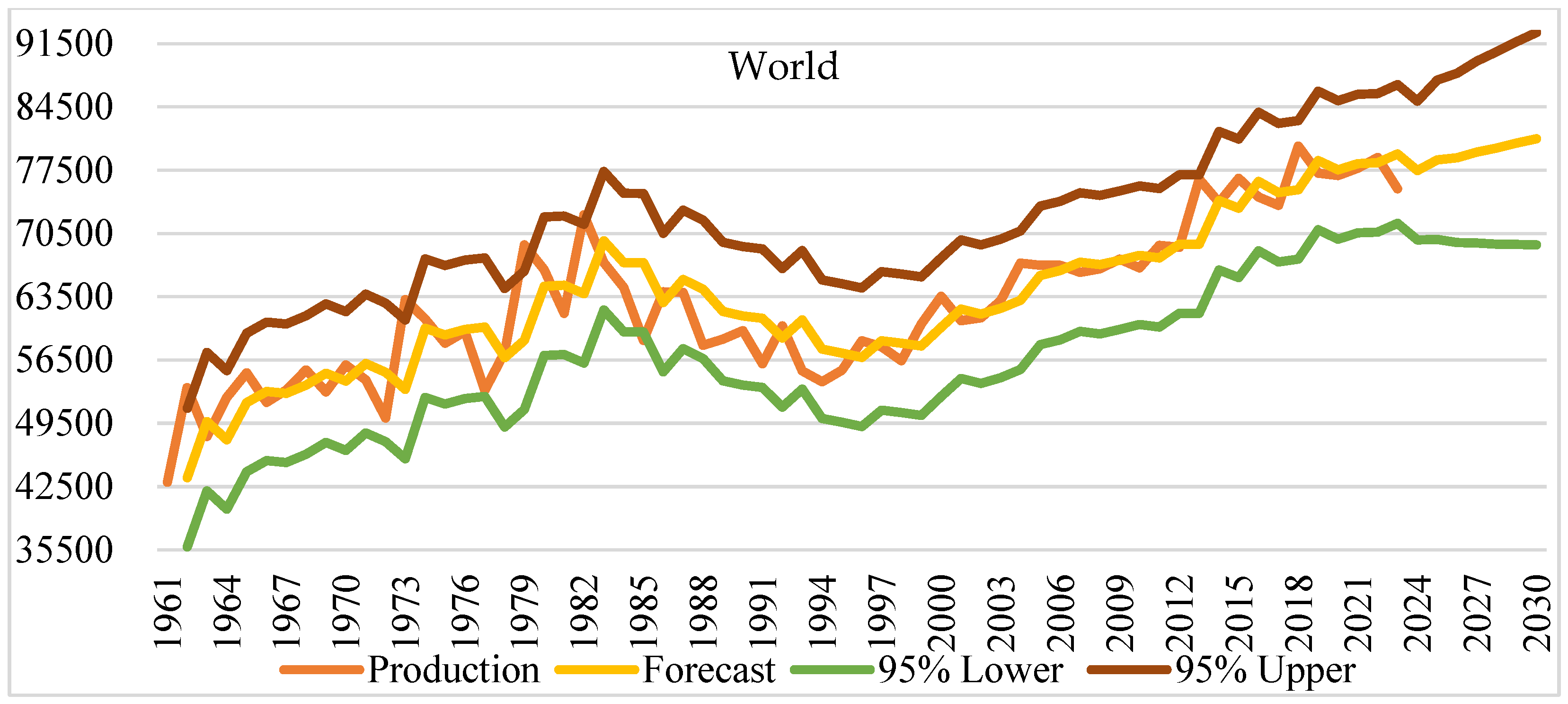
Grape production, which was recorded as 42.99 million tons in 1961, has fluctuated over the years and reached 75.44 million tons in 2023, with a compound annual growth rate of 0.89% in 63 years. During this period, various factors such as climatic conditions, developments in agricultural technologies and policies in producing countries had an impact on production. According to projections based on the ARIMA(1,1,2) model, global grape production is expected to increase steadily in the 2024–2030 period, reaching 77.46, 78.64, 78.87, 79.50, 79.96, 80.50 and 80.99 million tons, respectively. Compared to the average for the 2019–2023 period, production in the 2024–2030 period continues its upward trend and the sector maintains its growth potential (Figure 1).

3.3. Current and Projected Grape Production in China for the Years 1961–2030

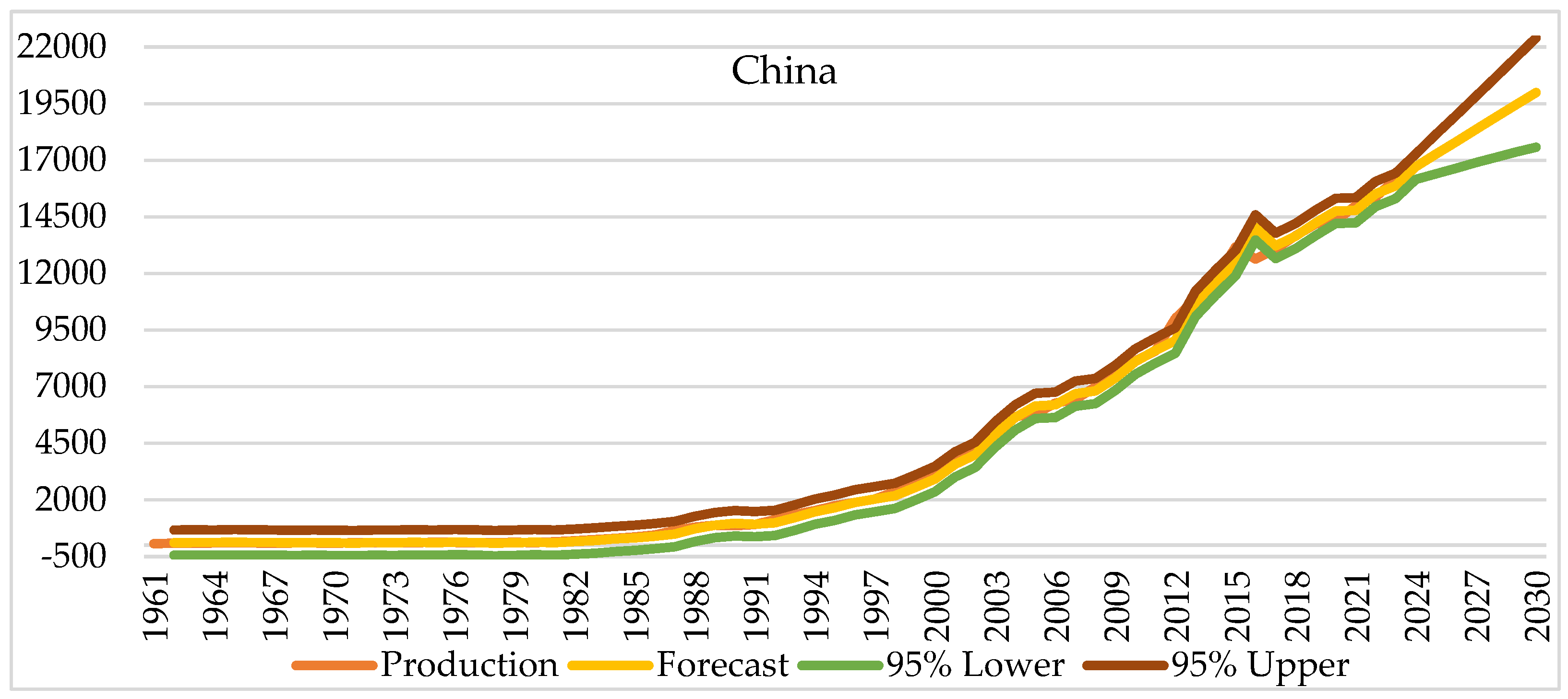
China’s grape production, which was only 70 thousand tons in 1961, has increased significantly in the last six decades, reaching 16.16 million tons in 2023, and with an integrated annual growth rate (CAGR) of 9.00% in 63 years, the country has become one of the world’s leading grape producers in this process. The agricultural policies implemented during this period, the development of irrigation infrastructure and the adoption of modern agricultural technologies have been effective in increasing production. Estimates based on the ARIMA(1,1,1) model predict that China’s grape production will follow a fluctuating course between 2024 and 2030. According to estimates, production will be approximately 16.71 million tons in 2024, 17.26 million tons in 2025, 17.80 million tons in 2026, 18.35 million tons in 2027, 18.90 million tons in 2028, 19.44 million tons in 2029 and 19.99 million tons in 2030. China’s production is expected to stabilize, supported by agricultural policies based on quality standards rather than land expansion. In addition, constraints that are structural in nature, such as variety restructuring and climate risks (for example, water scarcity in key regions), suggest that the industry is moving from a high-growth phase into a period of market maturity. Compared to the 2017–2023 period, a limited increase or stagnation in production is expected in the 2024–2030 period. This indicates that the rate of production growth is slowing down and the market is approaching saturation (Figure 2).

3.4. Current and Projected Grape Production in Italy for 1961–2030

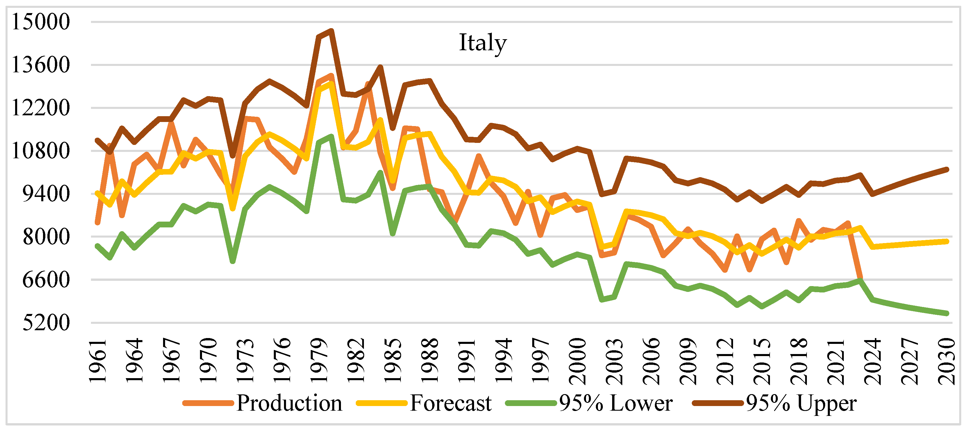
Italy’s grape production, which was only 8.47 million tons in 1961, increased to 13 million tons in the 1980s, but followed a generally fluctuating course in the following years. Since the 1990s, structural problems such as instability in production, climate change, changes in agricultural support and inadequate rural development led to a decline in production to 6.67 million tons in 2023. Despite a modest CAGR of 0.38% in 63 years, it is one of the world’s most important producers. According to the ARIMAX(1,0,1) model, Italy’s grape production is expected to increase steadily from 7.67 million tons in 2024 to 7.84 million tons by 2030, as shown in Figure 3.

3.5. Current and Projected Grape Production in France for the Years 1961–2030

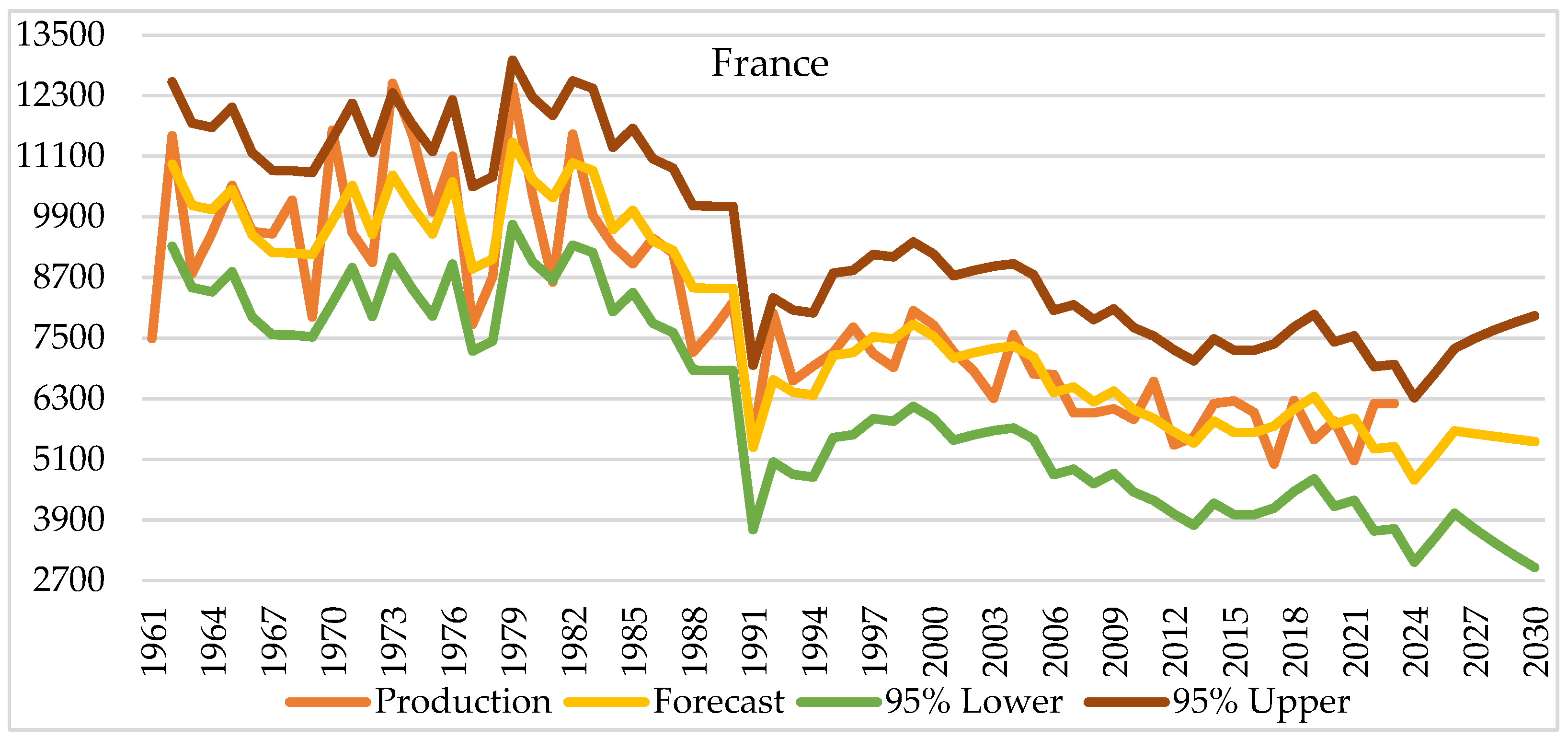
France’s grape production, which was approximately 7.49 million tons in 1961, peaked in the 1970s and 1980s, occasionally exceeding 12 million tons, but in the following years, due to climate change, land use changes and agricultural policies, it exhibited a fluctuating and generally decreasing trend. The decline in production, particularly since the 2000s, is striking, with output falling to approximately 6.21 million tons in 2023. Nevertheless, due to a long-term CAGR of 0.30% over the 63-year period, it maintains its position as one of the world’s most important producers. According to estimates based on the ARIMAX(0,1,3) model, France’s grape production amounts in the 2024–2030 period are projected as 4.69, 5.16, 5.66, 5.61, 5.57, 5.50 and 5.45 million tons, respectively (Figure 4).

3.6. Current and Projected Grape Production in Spain for the Years 1961–2030

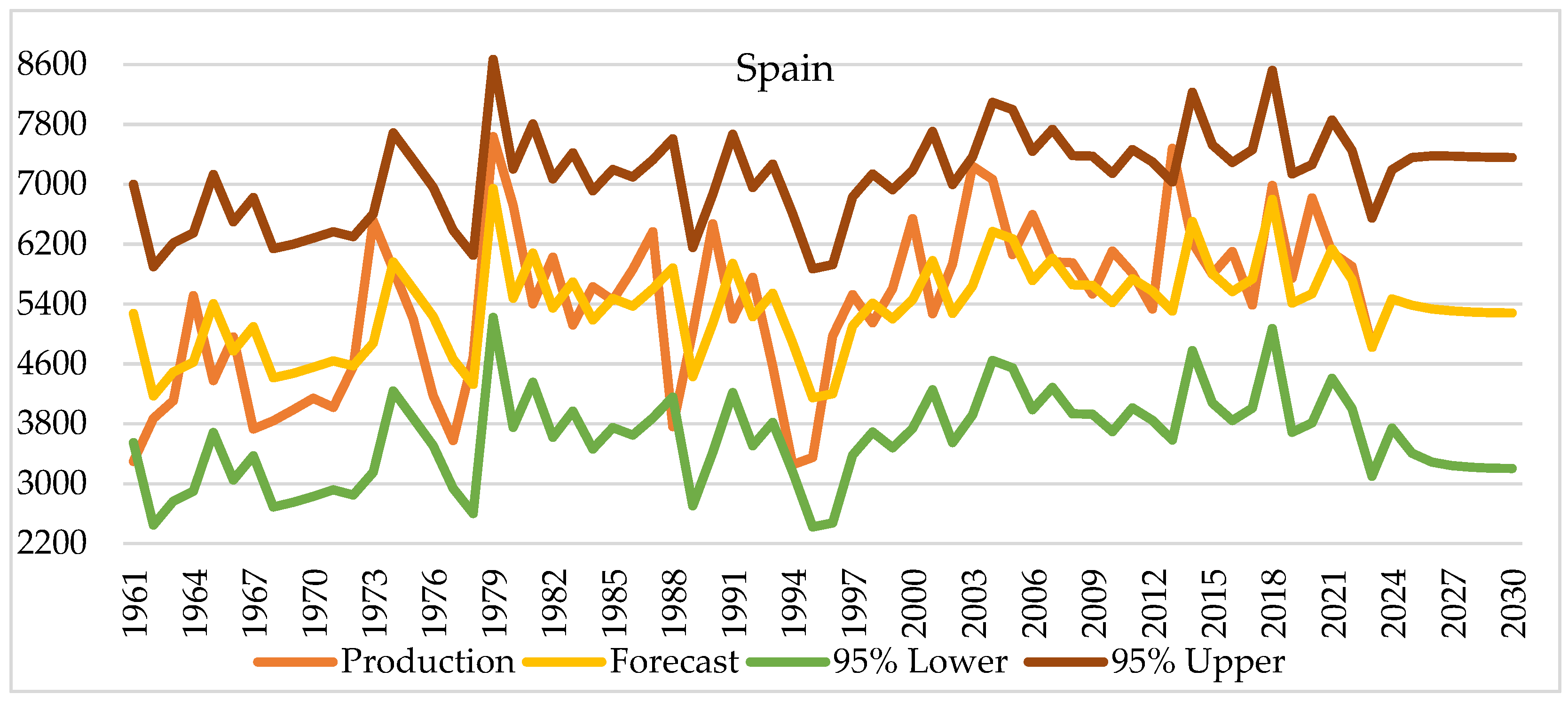
Spain’s grape production, which was approximately 3.30 million tons in 1961, showed a significant increase, reaching 7.6 million tons in the 1980s. However, production has fluctuated in the following years; environmental and structural factors, especially drought, depletion of water resources and changes in agricultural policies, have affected production levels. While production decreased significantly in 2023 to 4.82 million tons, the CAGR over 63 years was determined as 0.61% (Figure 5).
According to estimates based on the ARIMAX(1,0,0) model, Spain’s grape production is expected to fluctuate and recover in the 2024–2030 period, with production expected to be 5.47, 5.38, 5.33, 5.31, 5.29, 5.28 and 5.28 million tons, respectively.

3.7. Current and Projected Grape Production in the USA for the Years 1961–2030

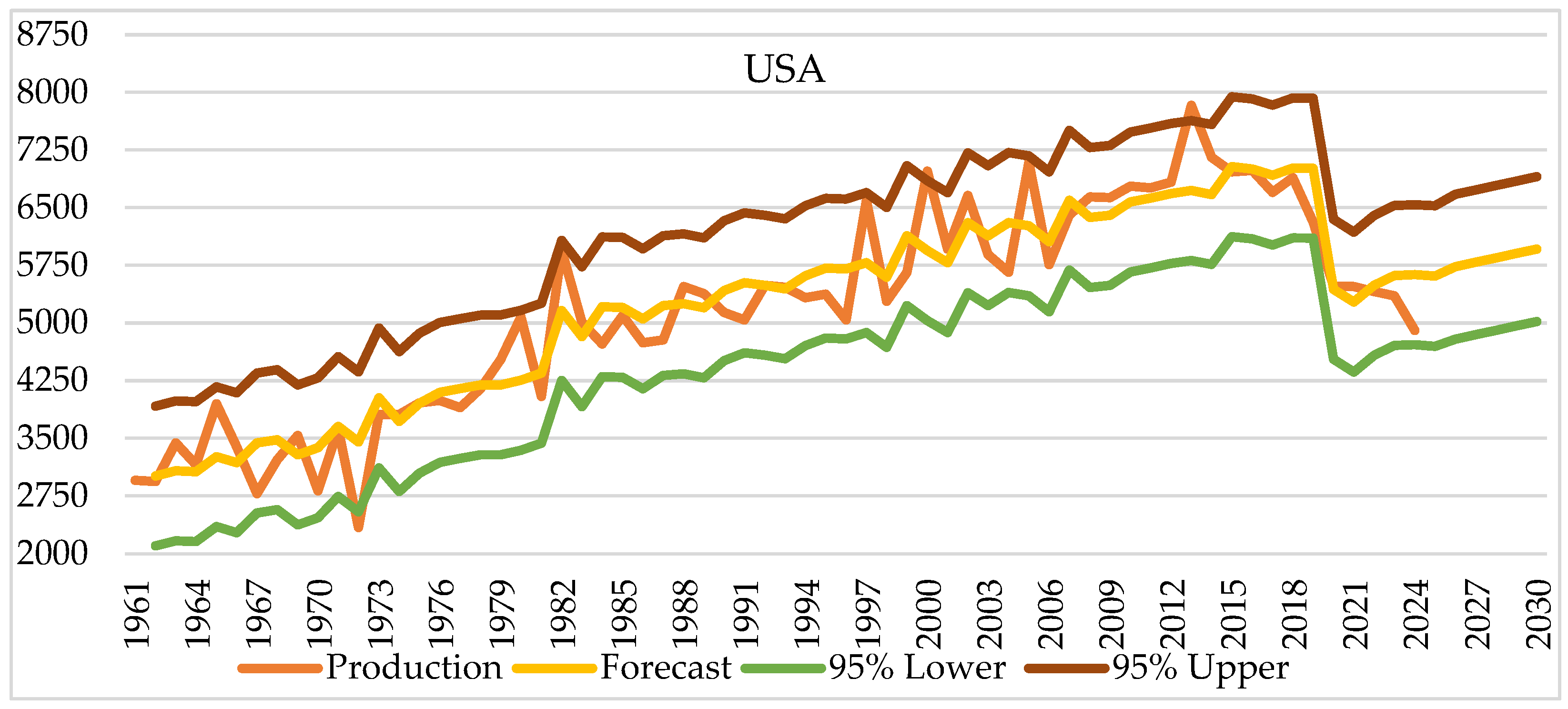
The grape production in the USA has generally increased from 1961 to 2013, peaking at 7.83 million tons in 2013. However, production started to decline after 2020, regressing to 5.36 million tons in 2023, and the CAGR has been determined as 0.95% in 63 years. According to ARIMAX(0,1,3) future projections, production is projected to be 5.63 million tons in 2024, 5.61 million tons in 2025, 5.73 million tons in 2026, 5.79 million tons in 2027, 5.85 million tons in 2028, 5.90 million tons in 2029, and 5.96 million tons in 2030. Although these data indicate that production will recover slightly, it is not expected to reach the high levels of the 2010s (Figure 6).

3.8. Current and Estimated Grape Production in Türkiye for the Years 1961–2030

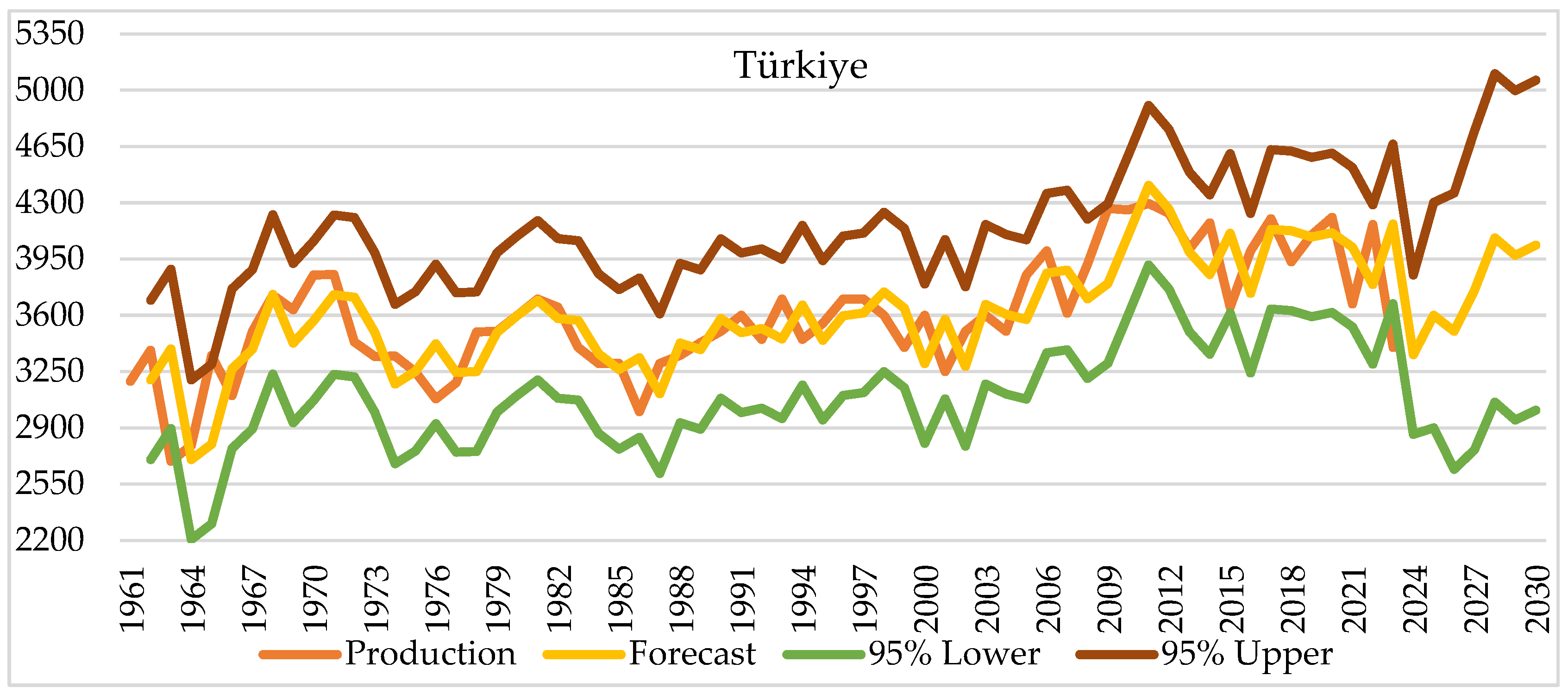
Production in Türkiye, which was 3.19 million tons in 1961, fluctuated over the years, stabilized in the 3.60–3.70 million tons band in the 1980s, and showed an increasing trend again after 2000. The country, which peaked at 4.27 million tons in 2009, regressed to 3.40 million tons in 2023, and the CAGR was determined as 0.10% in 63 years. According to ARIMA(4,1,5) estimates, production is expected to be 3.35 million tons in 2024, 3.60 million tons in 2025, 3.50 million tons in 2026, 3.76 million tons in 2027, 4.08 million tons in 2028, 3.97 million tons in 2029, and 4.04 million tons in 2030. These forecasts signal a short-term recovery in production but remain below previous peaks (Figure 7).

3.9. Current and Projected Grape Production in India for the Years 1961–2030

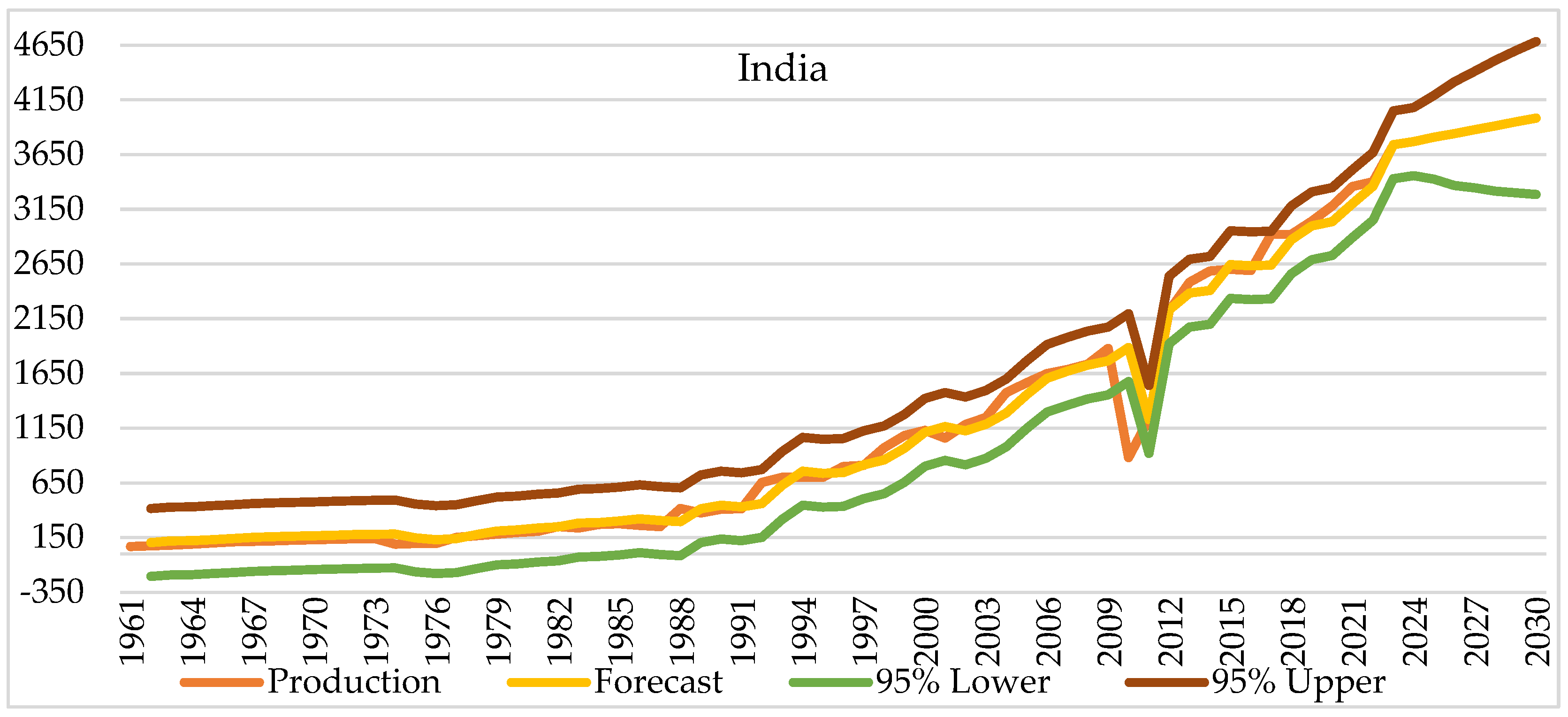
India’s grape production was only 70 thousand tons in 1961, but especially after 1990, rapid growth was remarkable, and it showed a great increase in the 2000s, and the production, which was 653 thousand tons in 1992, reached 1.25 million tons in 2003, 2.48 million tons in 2013, 3.18 million tons in 2020 and 3.74 million tons in 2023, and the CAGR in 63 years was determined as 6.52%. According to ARIMAX(1,1,0) estimates, grape production is expected to be 3.77 million tons in 2024, 3.81 million tons in 2025, 3.84 million tons in 2026, 3.88 million tons in 2027, 3.91 million tons in 2028, 3.95 million tons in 2029, and 3.98 million tons in 2030 (Figure 8).

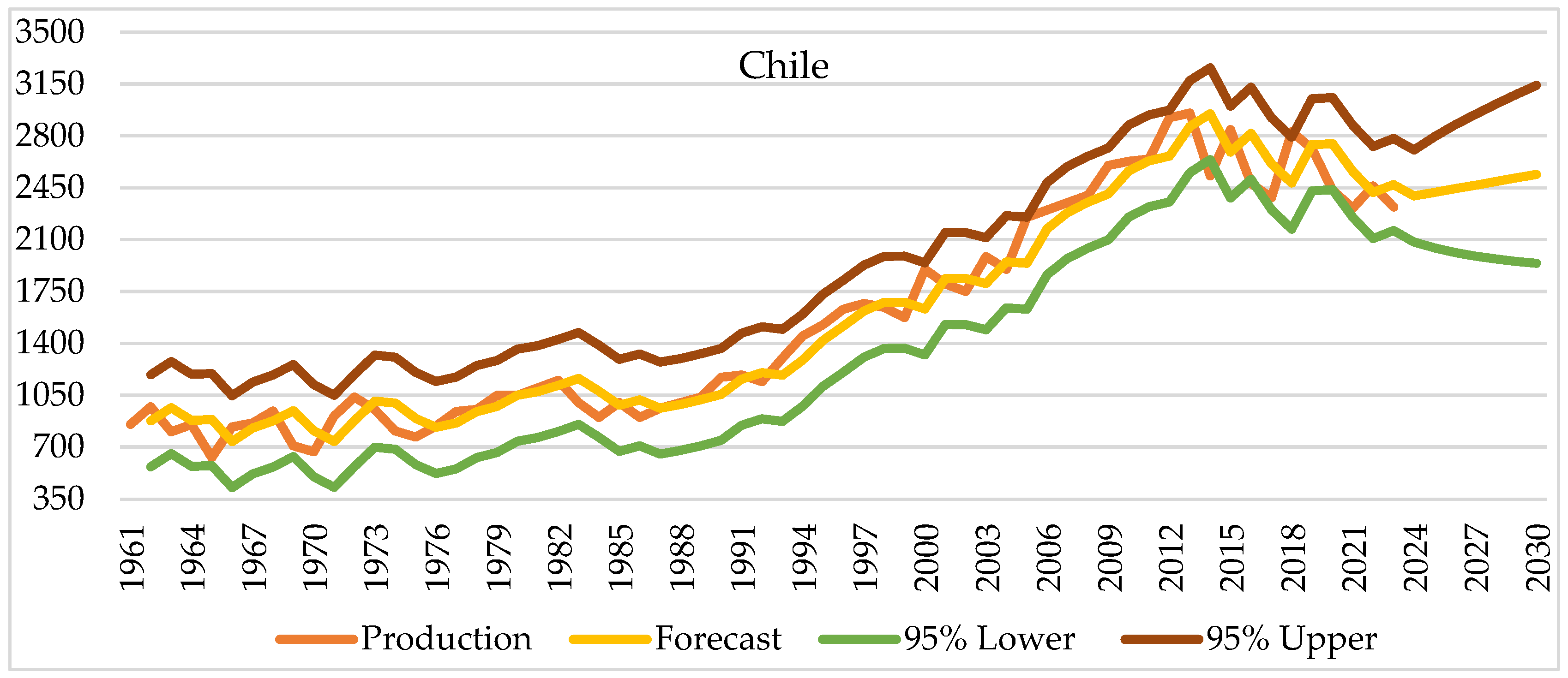
3.10. Current and Estimated Grape Production in Chile for the Years 1961–2030

Chile’s grape production was 853 thousand tons in 1961, and showed a fluctuating increase over the years, peaking at 2.92 million tons in 2012. Production tended to decline in the following years, falling to 2.55 million tons in 2023, but the CAGR over 63 years was determined as 1.75%. According to the ARIMA(0,1,1) model, production is projected to be 2.39 million tons in 2024, 2.42 million tons in 2025, 2.44 million tons in 2026, 2.47 million tons in 2027, 2.49 million tons in 2028, 2.52 million tons in 2029, and 2.54 million tons in 2030. These estimates reveal that Chile’s grape production will gradually increase over the next seven years but will not reach the highest levels in the past (Figure 9).

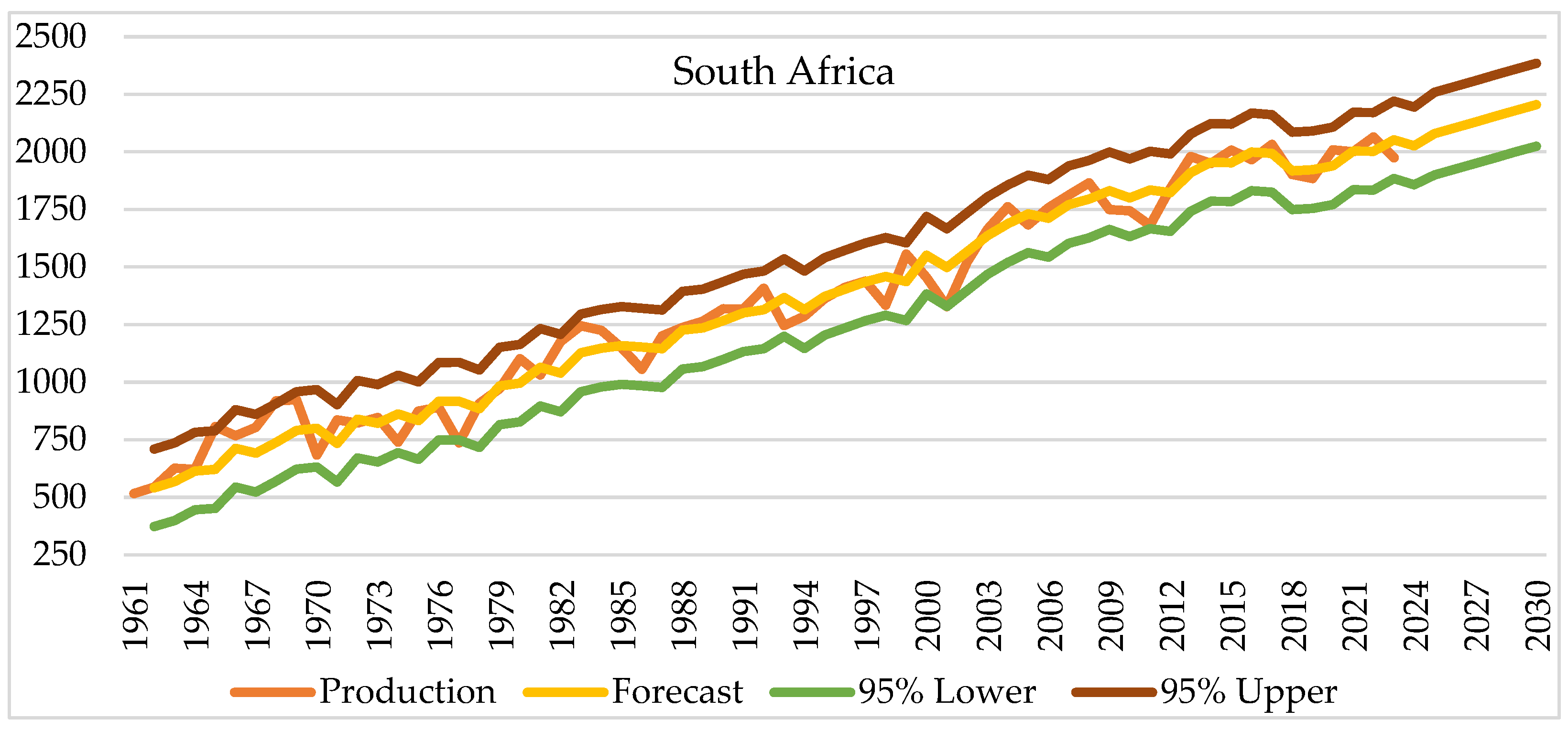
3.11. Current and Projected Grape Production in South Africa for the Years 1961–2030

South Africa’s grape production was 0.52 million tons in 1961, but has increased steadily over the years, approaching 1.10 million tons in 1980, 1.32 million tons in 1990, 1.45 million tons in 2000, 1.74 million tons in 2010, and 2.08 million tons in 2020. Production is expected to be 2.06 million tons in 2022 and 1.97 million tons in 2023, with a CAGR of 2.15% over 63 years. According to the ARIMAX(0,1,2) model, production is predicted to be 2.03 million tons in 2024, 2.08 million tons in 2025, 2.10 million tons in 2026, 2.13 million tons in 2027, 2.15 million tons in 2028, 2.18 million tons in 2029, and 2.20 million tons in 2030. These estimates demonstrate that South Africa exhibits a highly stable and resilient growth trend in grape production, suggesting that output exceeding the 2-million-ton threshold will become permanent in the coming years (Figure 10).

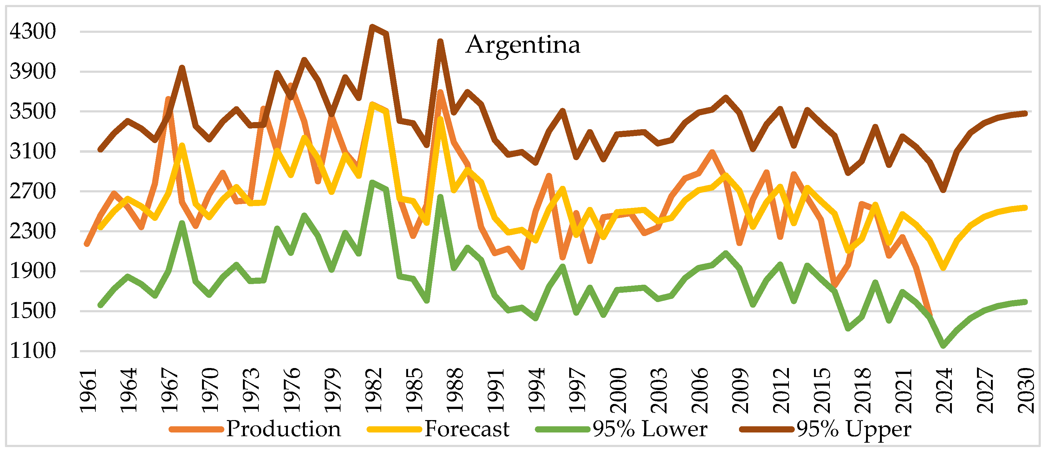
3.12. Current and Estimated Grape Production in Argentina for the Years 1961–2030

Argentina’s grape production was 2.17 million tons in 1961, followed by a fluctuating course in the 1980s and 1990s, and reached a peak of 3.09 million tons in 2007. In the 2020s, there was a significant decrease in production, with production falling to 1.46 million tons in 2023, with a CAGR of 0.64% over 63 years. According to ARIMAX(0,1,2) estimates, production is expected to be 1.93 million tons in 2024, 2.21 million tons in 2025, 2.36 million tons in 2026, 2.44 million tons in 2027, 2.49 million tons in 2028, 2.52 million tons in 2029, and 2.54 million tons in 2030. These estimates suggest that Argentina’s grape production shows a steady upward trend in the long-term, reflecting a consistent recovery over the coming years (Figure 11).

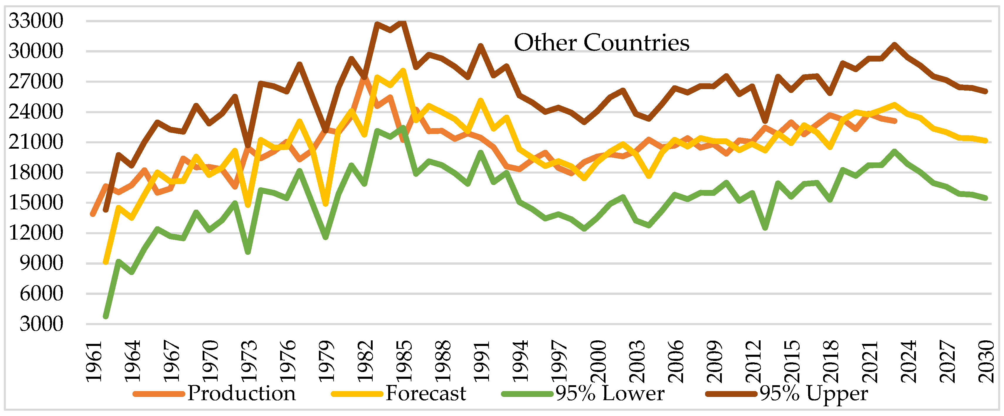
3.13. Current and Projected Grape Production in Other Countries for the Years 1961–2030

Total grape production in other countries was recorded as 13.91 million tons in 1961, and production reached 22–27 million tons in the 1980s. In the period after 2012, fluctuating but generally high production levels were maintained. Production was realized as 23.11 million tons in 2023, and the compound annual growth rate was realized as 0.81% in 63 years. Based on the residual calculation (World total minus the top 10 countries), production is projected to be 23.81 million tons in 2024, 23.42 million tons in 2025, 22.35 million tons in 2026, 22.01 million tons in 2027, 21.44 million tons in 2028, 21.40 million tons in 2029, and 21.16 million tons in 2030. These estimates suggest that grape production in other countries remains stable, albeit showing a slight downward trend over the next seven years (Figure 12).
The share of other countries in the 2020–2023 period is 30.08%, indicating that there are also important producers outside the top 10 countries in world grape production. In the 2020–2023 period, approximately 19.04% of world grape production was realized by 12 countries outside the top 10 producing countries. In this group, Uzbekistan leads with a share of 2.25% with an annual average production of 1.92 million tons. It is followed by high-production countries such as Brazil (2.10%), Egypt (2.09%), Australia (2.09%) and Iran (2.08%). Germany (1.54%) is one of the prominent mid-level producers. On the other hand, Afghanistan and Portugal are positioned in the middle-lower segment with shares below 1.2%. It is seen that countries such as Romania, Peru, the Russian Federation and Greece have shares around 1% [15].

3.14. Long-Term Analysis of Competitiveness in Global Grape Markets

Table 2 shows the ARIMA forecasts for 2024–2030, reflecting the changes in production in major global grape-producing countries. The long-term trends of the five-country concentration ratio (CR5) reveal the sector’s evolution from a Eurocentric structure to a more globalized production network from 1961 to 2030. Traditional producers (Italy, France and Spain) accounted for 59.23% of total output in the 1960s, but market projections suggest a shrinkage to 52.02% by 2030, reflecting geographical expansion and increased global competition. The most basic structural change occurred in 2011, when the first place was overtaken by China from Italy, France, USA and Spain. This structural reallocation dislodged historical major producers such as Türkiye and the USSR from the top-five rankings. Simultaneously, the global market has become increasingly less concentrated, as shown in the decline of the HHI from 0.11 to 0.09, meaning the global viticulture industry has become a geographically dispersed and strategically diversified ecosystem.

3.15. Future Production Outlook (2024–2030)

Table 3 summarizes ARIMA and ARIMAX forecast results during the period of 2024–2030. The models predict a continued rise in global grape production with values ranging between 77.46 and 80.99 million tons from 2024 to 2030. The most prominent performers of this period are China, which is expected to boost its production by around 3 million tons to 19.99 million tons, and Argentina, which is recovering considerably. Traditional European producers like Italy and Spain are likely to see a small reduction in their production capacity. Production capacities in France, the United States, and India are expected to remain stable or increase. Türkiye will cross the 4 million tons mark with a fluctuating but increasing trend and consolidate its strategic position in the global supply. In general, the picture is one of expansion of the world grape market on the supply side through the end of the next decade, with production growth in the leading countries as well as in the “Others” category.

4. Discussion

In the absence of peer-reviewed forecasting studies in viticulture, we partially derived our production benchmarks from commercial reports [49]. Our predictions follow the upward trend of [49], but with a lower compound annual growth rate (CAGR) of 0.76% instead of 0.84%, with 80.99 million tons in 2030. Both models, despite the difference in methodology, confirm the transition of the sector from stagnation to a phase of steady growth. This stability is also supported by historical yield averages from FAO [15] (2018–2023) that estimate a normalized production of 76.9 million tons, confirming the low deviation of our estimates. The market exhibits a high level of concentration in terms of trade dynamics. The main consumption centers, the USA (18.70%), Germany (8.30%), the Netherlands (7.15%), and the UK (6.94%), represent 56.21% of world imports [50]. In the horticultural case, this growth path is determined by technological and physiological progress, not simply by statistical momentum. In the USA, disease-resistant genotypes [51] reduce the losses of yield caused by endemic pathogens, and in Europe (France, Germany, Italy and Spain), resistant cultivars reduce the dependency on pesticides by 50–80% [52]. Meanwhile, Chinese viticulture is developing physiological buffers against climate-induced volatility through CRISPR-based gene editing, precision canopy management and cold-resistant varieties [53,54]. These structural and agronomical innovations can efficiently stabilize the annual yields, thus allowing a strong and sustained production uptrend in the face of continuing environmental stressors.
For China, our empirical forecasts are compatible with the growing path in [49] but deliver a more sophisticated path with the optimized ARIMA(1,1,1) framework. Our models are much more sensitive to changes from year to year than broader models, which tend to smooth out short-term volatility and focus on long-term trends. Hence, we expect production to grow steadily from 16.71 million tons in 2024 to 19.99 million tons by 2030. This expansion is driven by China’s aggressive adoption of viticultural innovations, including CRISPR-based gene editing, genomic selection [53], and cold-resistant varieties [54] that buffer crops from extreme climatic shocks. We also perform an external validation of our framework by comparing the 2024 forecast with real data from FAO [15]. Our model has excellent predictive accuracy with only a −0.65% deviation. This precision highlights the framework’s superior capability to capture technology-driven agricultural dynamics compared to more conservative machine learning alternatives.
According to the ARIMAX(1,0,1) model, the Italian grape production would recover from 6.67 million metric tons in 2023 to a stable range of 7.67–7.84 million tons for 2024–2030. We purposely selected this model, which did not require first-order differencing (d = 0), in order to avoid imposing a downward trend based solely on the anomaly of 2023. The historic 2023 decline was not a structural contraction but rather the consequence of transitory biological shocks, notably catastrophic downy mildew outbreaks and climate-intensified disease pressures, that acutely disrupted the northern Italy viticulture [10]. From an agronomic point of view, this trajectory is a physiological recovery towards historical baselines and not a structural decline. The real Italian 2024 production of 7.64 million metric tons [55] supports this conclusion, exactly matching our ARIMAX(1,0,1) forecast with a difference of only 0.40%. Although high-resolution UAV-based mapping [56] can accurately estimate intra-seasonal yield, these models typically lack the predictive power for medium-term forecasting. The results confirm that the ARIMAX architecture proposed here, despite the methodological differences, presents structural consistency and robust forecasting accuracy for the Italian viticulture.
The ARIMAX(0,1,3) model forecasts that France’s grape production will rise from 4.69 million metric tons in 2024 to a peak of 5.66 million metric tons in 2026, subsequently leveling off to 5.45 million metric tons by 2030. On the other hand, alternative market reports [49] provide more conservative estimates due to a lower baseline and different modeling assumptions. In contrast to the Italian model’s stationary approach, first-order differencing (d = 1) was strictly required here to integrate France’s ongoing structural contraction, driven by the state-subsidized, large-scale uprooting of vineyards in Bordeaux. The robustness of this model is strongly validated by France’s actual 2024 production of 4.75 million metric tons [54], showing a minimal variance of merely −1.17%. From a horticultural perspective, this predictive accuracy is very meaningful as the model assimilates both these permanent areal changes and acute phytosanitary shocks. In particular, it reflects the strong downward pressures caused by late spring frosts, hail, and delayed vine development, as well as the catastrophic outbreaks of downy mildew and poor fruit sets that devastated French harvest volumes in 2024, as recorded by Decanter [57]. The presented ARIMAX framework, by filtering out these concomitant climatic anomalies and structural changes, proposes a biologically based and realistic trajectory for French viticulture.
The ARIMAX(1,0,0) model forecasts that Spanish grape production will rebound and stabilize between 5.47 million metric tons in 2024 and 5.28 million metric tons in 2030. This architecture was largely a response to the steep decline in production in 2023 to 4.82 million metric tons. From a viticultural and ecological perspective, this historic drop was a direct result of intense drought stress and increasing climate variability across the Iberian Peninsula, which severely changed the annual vineyard yield dynamics, as discussed in Spanish viticulture by Cubillas et al. [58]. The non-differenced structure (d = 0) does not over-penalize the forecast based on this extreme outlier but rather captures a mean-reverting recovery that reflects the agricultural sector’s climate resilience and a physiological return toward historical baseline production levels. Conversely, alternative industry reports [49] predict a static trend, estimating 6.08 million metric tons in 2024 and sustaining a rigid projection of 6.07 million metric tons from 2025 to 2028. The difference is mainly attributed to methodological variations, since the framework in [49] is trend-free, assuming static production environments and hence almost identical annual outputs. According to Eurostat [55], the actual grape production in 2024 was 5.39 million metric tons. Our ARIMAX prediction is 5.47 million metric tons with a small variance of just 1.51% relative to this official statistic, which further confirms the model’s ability to exclude transient shocks caused by climate without losing structural forecasting accuracy.
The ARIMAX(0,1,3) model presents a mild increase in US grape production from 5.63 to 5.96 million metric tons from 2024 to 2030, less than the prediction of 6.28–6.16 million tons by [49]. The real 2024 production (4.90 million tons as per FAO [15,59]) is an upward deviation of 14.85% from our model. But this divergence is not a statistical failure but rather the result of a significant structural shift: our model shows the historical ‘natural’ trend of production, while the market deliberately restrained actual volumes. US growers have reacted to changing consumer tastes and a structural oversupply by limiting harvests to avoid price collapses, a strategy confirmed by a 7% reduction in California vineyards [59,60] and industry-wide supply management reports, following a decade of contraction from the 2013 peak (7.83 million tons; 18,571 kg/ha) (Silicon Valley Bank) [61]. Hence, our model captures the underlying productive potential well, while actual output is determined by producer-driven adjustments to restore market equilibrium. Looking ahead, as initiatives like diversified grape-based industries and federal procurement programs come back to balance the demand–supply equation, production is expected to converge on the optimal growth path predicted by our model.
Türkiye’s viticulture sector has been stagnant for a long time, with just 0.10% compound annual growth rate (CAGR) over a 63-year period. This trend is, as noted by Soylemezoglu et al. [62], a reflection of structural constraints such as a 7.8% decrease in vineyard area between 2018 and 2022, as growers switched to competing crops such as olives and maize. Productivity is also affected by 40% reduction in sapling production and an acute shortage of disease-free planting materials. The ARIMA(4,1,5) model estimated an increase in production from 3.35 million tons in 2024 to 4.04 million tons in 2030. The model is robust, with an average estimated output of 4.02 million tons for 2016–2023, close to the reported 3.96 million tons and above the 3.87 million ton benchmark [63]. In addition, our projection for 2030 (4.04 million tons) is consistent with the strategic efficiency targets suggested by Soylemezoglu et al. [62]. Most importantly, our 2024 prediction (3.35 million tons) was more accurate than other estimates [63] and close to the actual production of 3.46 million tons. This accuracy reflects the ARIMA model’s ability to incorporate the transitory biological and climatic shocks that are normally averaged out by broad econometric trend lines.
The ARIMAX(1,1,0) model is validated on the basis of the consistency of the observed market trends in India. FAO data indicate a stable trend structure; average yields are constantly 21,000–22,000 kg/ha (2013–2024). From a horticultural standpoint, such stability indicates a mature agronomic equilibrium capable of handling climate-induced variability through efficient stress management. Even though tropical viticulture is subjected to severe abiotic stresses such as high temperature, drought and salinity [64], India still produces consistently using modern technologies such as strategic canopy management, stress-tolerant rootstocks and protective netting. This resilience is the basis for the steady growth of the sector, supported by an increase in harvested area from 118,000 to 179,629 ha. Our model is able to describe the biological and structural dynamics well, and for 2024 we estimate a production of 3.90 million tons with a deviation from the FAO reports of only 3.47%. The other literature [21,49] also supports this and independently confirms a steady growth trend to the 3.7 million tons mark by 2026.
ARIMA(0,1,1) model forecasts that Chilean grape production will increase from 2.39 million tons in 2024 to 2.54 million tons in 2030. This positive trend suggests that the viticultural landscape is resilient, both structurally and geographically, to the abiotic stress of climate change, i.e., the 0.83 °C increase in maximum temperatures and 20–30% decrease in winter precipitation described by Ríos-Núñez et al. [65], and that the viticultural landscapes are able to adapt to these changes. The sector is responding to these challenges with multiple strategies, such as cold-climate viticulture extending to southern and coastal areas south of the 38th parallel, late pruning to preserve fruit acidity, artificial shading to manage radiation, and the use of drought-resistant rootstocks such as R32. Although study [49] offers higher estimates of between 2.86 and 2.94 million tons for the period 2024–2028, data from [15] indicate that Chile’s actual production in 2024 was 2.4 million tons. Compared to this official figure, our model’s estimate of 2.39 million tons shows a minimal deviation of −2.43%, proving that it successfully captures the biological dynamics shaped by technological and regional innovations, thereby validating the model as a reliable tool for supply projections in the international grape trade.
The ARIMAX(0,1,2) model predicts a steady upward trajectory to 2.15 million tons in 2030, underscoring the structural and biological resilience of South Africa’s viticulture industry. Unlike purely autoregressive frameworks such as the ARIMA(2,1,3) model [42], which wrongly predicts a decline by not incorporating long-term adaptations, our model includes exogenous variables such as phenology and climate-driven yield constraints. This provides a physiologically based interpretation of the sector dynamics. As shown by Myeki et al. [66], the industry is very sensitive to climate (0.09% output loss per 1 °C increase), with extreme weather threatening the key traits of berry size and color in key production centers. Myeki et al. [66] attribute the decline in total factor productivity (4.29% per year, 2010–2020) to innovation lagging behind climate. Our growth outlook is a reflection of the industry’s rebound through strategic shifts such as the adoption of drought-tolerant, high-demand seedless varieties and precision water management. So, our model is statistically sound, based on real-world horticultural dynamics and a robust tool for agricultural planning.
The ARIMAX(0,1,2) model forecasts a steady increase in Argentine grape production from 1.93 to 2.54 million tons by 2030, showing a minimal 0.84% deviation from actual 2024 data. This outperforms previous estimates [49], which projected a stagnant production level of 2.49–2.50 million tons by failing to account for the sector’s ongoing structural changes. Argentina, contributing 9% of global production, is undergoing a profound climate-driven transformation. Ríos-Núñez et al. [65] demonstrate that projected temperature rises of up to 3.2 °C by the end of the century are accelerating vine phenology, with each 1 °C increase advancing the harvest by 7.4 days. This thermal shift is detrimental to critical horticultural traits—such as acidity and color—in key varieties like Malbec and Pinot Noir. To maintain quality, the industry is transitioning toward robust Criolla cultivars and relocating vineyards to higher elevations or cooler southern regions like Patagonia and Salta [65]. These geographical adaptations, coupled with technological interventions such as precision irrigation and early warning systems, suggest that our ARIMAX model’s projection is more aligned with the industry’s actual evolutionary trajectory than traditional autoregressive frameworks.
As of 2024, global grape production is estimated to be approximately 77.46 million tons. Of this total, the top ten grape-producing countries account for 54.44 million tons, while the remaining 23 million tons are produced by other countries. Among these other producers, Uzbekistan, Brazil, Egypt, Australia, Iran, Germany, Afghanistan, and Portugal stand out as significant contributors.
Comparative assessments conducted across 12 distinct nations corroborate the short- and middle-term forecasting efficacy of the ARIMA model in this work. These studies indicate that ARIMAX models provide greater accuracy in short-term forecasts compared to fixed-estimate and trend-based methods, mostly owing to their capacity to incorporate recent changes in time series data. This advantage arises from the model’s ability to rapidly adapt to abrupt changes in output, seasonal variations, and prevailing market circumstances. Consequently, the results of this research align with the structural characteristics of the ARIMA model and the outcomes of multi-country studies, affirming that ARIMAX is a dependable and efficient approach for short- and middle-term forecasting of grape output.

5. Conclusions

Grapes are an important product worldwide, used for both fresh markets and processed products, such as raisins, wine, and juice. However, specific climatic, soil, and technical conditions restrict grape growing to certain regions and countries. The top ten grape-producing countries are expected to produce 73% of the world’s grapes in 2024–2030, led by China, Italy, France, Spain, and the USA. India, Türkiye, Chile, South Africa, and Argentina also play important roles. The top five countries account for approximately 54% of the total production, while the next five countries are expected to contribute another 19%. The remaining 27% is largely produced by countries such as Uzbekistan, Brazil, Egypt, Australia, Iran, Germany, Afghanistan, and Portugal, which are becoming more significant players in the global market. The HHI is at a low level of 0.08 despite a large share of production being concentrated in countries, indicating a competitive market structure. Policymakers should use these forecasts to promote climate-resilient viticulture technology, diversify supply chains to reduce regional vulnerabilities, and disseminate these results to enhance long-term food security. Key wine producers are deploying climate-resilient grape varieties, precision irrigation, and digital agriculture technologies to adapt to climate change challenges, including water scarcity, rising temperatures, and increasing disease pressure. This helps them improve quality and sustainability while ensuring yield stability. These adaptive strategies are vital for maintaining a competitive edge in changing markets. As a result, production alone is no longer sufficient to guarantee success in the global grape sector. Producers must innovate, adapt to environmental changes, and provide high-quality, sustainable products. In our study, we mainly used the ARIMA model for prediction. ARIMA-based models have some limitations, such as linear constraints, structural breaks during COVID-19, reliability of data in some regions, and short forecast horizons. Hence, we also predicted for many countries using the ARIMAX model, which includes exogenous variables in the process. However, future work on hybrid machine learning models with data access issues, integration of climate scenarios (RCPs) deep inside the model, and analysis of harvest area and yield as separate components can improve long-term forecasting accuracy and strategic planning. This will help grape-producing countries make better decisions and be more resilient in the long-term.

Author Contributions

M.K. and A.S.U.; methodology, M.K. and A.S.U.; software, A.S.U.; validation, E.G. and A.S.U.; formal analysis, M.K.; investigation, A.S.U. and E.G.; resources, A.S.U.; data curation, M.K., A.S.U. and E.G.; writing—original draft preparation, A.S.U.; writing—review and editing, M.K.; visualization, E.G.; supervision, A.S.U.; project administration, M.K.; funding acquisition, M.K. All authors have read and agreed to the published version of the manuscript.

Funding

This research received no external funding.

Institutional Review Board Statement

Not applicable.

Informed Consent Statement

Not applicable.

Data Availability Statement

The original contributions presented in this study are included in the article. Further inquiries can be directed to the corresponding author.

Conflicts of Interest

The authors declare that they have no conflicts of interest.

References

  1. Ataseven, Y.; Arisoy, H.; Gurer, B.; Demirdogen, A.; Olhan, N.O.E. Global Agricultural Policies and Their Reflections on Turkish Agriculture. In Proceedings of the 9th Technical Congress of Agricultural Engineering in Turkey, Ankara, Turkey, 13–17 January 2020; Volume 1, pp. 11–36. Available online: https://api2.zmo.org.tr/uploads/portal/resimler/ekler/3e99ecaf98a5e17_ek.pdf (accessed on 26 March 2025). (In Turkish)
  2. Riekötter, N. Sustainability in Viticulture-Agroforestry and Organic Wine Production in the Mosel Region, Germany. Ph.D. Thesis, Philipps-Universität Marburg, Marburg, Germany, 2023. [Google Scholar]
  3. Kupe, M. Recent Changes and Current Situation in Turkish Viticulture. Sustainability from Seed to Table: Some Suggestions for Agricultural Resource Consumption. İKSAD Publ. 2021, 7, 147–174. Available online: https://iksadyayinevi.com/wp-content/uploads/2021/12/TOHUMDAN-SOFRAYA-SURDURULEBILIRLIK-TARIMSAL-KAYNAK-TUKETIMI-ICIN-BAZI-ONERILER.pdf (accessed on 26 March 2026).
  4. Siller-Sánchez, A.; Luna-Sánchez, K.A.; Bautista-Hernández, I.; Chávez-González, M.L. Use of Grape Pomace from the Wine Industry for the Extraction of Valuable Compounds with potential use in the Food Industry. Cur. Food Sci. Technol. Rep. 2024, 2, 7–16. [Google Scholar] [CrossRef]
  5. TURKSTAT. Turkish Statistical Institute. Türkiye Grape Production Data. Available online: https://data.tuik.gov.tr/ (accessed on 20 July 2025).
  6. Dal Santo, S.; Zenoni, S.; Sandri, M.; De Lorenzis, G.; Magris, G.; De Paoli, E.; Pezzotti, M. Grapevine field experiments reveal the contribution of genotype, the influence of environment and the effect of their interaction (G×E) on the berry transcriptome. Plant J. 2018, 93, 1143–1159. [Google Scholar] [CrossRef] [PubMed]
  7. Santos, J.A.; Fraga, H.; Malheiro, A.C.; Moutinho-Pereira, J.; Dinis, L.T.; Correia, C.; Moriondo, M.; Leolini, L.; Dibari, C.; Costafreda-Aumedes, S.; et al. A review of the potential climate change impacts and adaptation options for European viticulture. Appl. Sci. 2020, 10, 3092. [Google Scholar] [CrossRef]
  8. Dominguez, D.L.; Cirrincione, M.A.; Deis, L.; Martínez, L.E. Impacts of climate change-induced temperature rise on phenology, physiology, and yield in three red grape cultivars: Malbec, Bonarda, and Syrah. Plants 2024, 13, 3219. [Google Scholar] [CrossRef]
  9. Sodini, M.; Callesen, T.; Canton, M.; Tezza, L.; Campos, F.B.; Zanotelli, D.; Tarolli, P.; Sivilotti, P.; Pitacco, A.; Tagliavini, M. Major threats caused by climate change to grapevine. Italus Hortus 2023, 30, 1–24. [Google Scholar] [CrossRef]
  10. Fishman, K. Winers or Losers: Assessing the Socio-Economic Impact of EU Regulations on Climate-Exacerbated Pests and Diseases in Northern Italian Viticulture. In Proceedings of the Claremont-UC Undergraduate Research Conference on the European Union, Claremont, CA, USA, 3–4 April 2025; Volume 1. [Google Scholar]
  11. Khadatkar, A.; Sawant, C.P.; Thorat, D.; Gupta, A.; Jadhav, S.; Gawande, D.; Magar, A.P. A comprehensive review on grapes (Vitis spp.) cultivation and its crop management. Discov. Agric. 2025, 3, 9. [Google Scholar] [CrossRef]
  12. Bayraktar, T.U.; Sengul, Z.; Altin, A. Evaluating Sustainability Practices in Viticulture Through a Comprehensive Study of Environmental, Social, and Economic Factors: A Case from Batman Province, Türkiye. Turk. J. Agric.-Food Sci. Technol. 2024, 12, 1696–1705. [Google Scholar] [CrossRef]
  13. Fandl, K.J. Regulatory policy and innovation in the wine industry: A comparative analysis of old and new world wine regulations. Am. Univ. Int. Law Rev. 2018, 34, 279. Available online: https://digitalcommons.wcl.american.edu/auilr/vol34/iss2/2/ (accessed on 26 March 2026).
  14. Cardell, M.F.; Amengual, A.; Romero, R. Future effects of climate change on the suitability of wine grape production across Europe. Reg. Environ. Change 2019, 19, 2299–2310. [Google Scholar] [CrossRef]
  15. FAOSTAT. Global Grape Production Statistics. Available online: http://www.fao.org/faostat/en/#data/QC (accessed on 24 June 2025).
  16. Pomarici, E.; Corsi, A.; Mazzarino, S.; Sardone, R. The Italian wine sector: Evolution, structure, competitiveness and future challenges of an enduring leader. Ital. Econ. J. 2021, 7, 259–295. [Google Scholar] [CrossRef]
  17. Ayuda, M.I.; Ferrer-Pérez, H.; Pinilla, V. A leader in an emerging new international market: The determinants of French wine exports, 1848–1938. Econ. Hist. Rev. 2020, 73, 703–729. [Google Scholar] [CrossRef]
  18. Alston, J.M.; Sambucci, O. Grapes in the world economy. In The Grape Genome; Springer: Cham, Switzerland, 2019; pp. 1–24. [Google Scholar] [CrossRef]
  19. García Juárez, H.D.; Montes Ninaquispe, J.C.; León Luyo, S.L.; Marquez Yauri, H.Y.; Mendoza Ocaña, C.E.; De La Cruz Ruiz, N.V.; Villanueva Butrón, G.V. Competitiveness and Diversification in Grape Exports: Keys to Their Sustainability in Global Markets. Agriculture 2025, 15, 1894. [Google Scholar] [CrossRef]
  20. Dressler, M. Meeting market and societal ambitions with new robust grape varietals: Sustainability, the green deal, and wineries’ resilience. Agriculture 2024, 14, 2138. [Google Scholar] [CrossRef]
  21. Ray, S.; Mishra, P.; Ayad, H.; Kumari, P.; Sharma, R.; Kumari, B.; Biswas, T. Prediction of fruit production in India: An econometric approach. J. Hort. Res. 2023, 31, 25–34. [Google Scholar] [CrossRef]
  22. Petrović, M.S.; Savić, B.V.; Jakšić, D.D. Forecast of planting vineyards with local grapevine varieties in the Republic of Serbia using the ARIMA models. Zb. Matice Srp. Prir. Nauk. 2024, 146, 129–142. [Google Scholar] [CrossRef]
  23. Andrade, C.B.; Moura-Bueno, J.M.; Comin, J.J.; Brunetto, G. Grape yield prediction models: Approaching different machine learning algorithms. Horticulturae 2023, 9, 1294. [Google Scholar] [CrossRef]
  24. Patil, N.; Bhise, A.; Tiwari, R.K. Fusion deep learning with pre-post harvest quality management of grapes within the realm of supply chain management. Sci. Temper. 2024, 15, 168–176. [Google Scholar] [CrossRef]
  25. Puga, G.; Anderson, K. Statistical methods in grape and wine research for quantifying the impact of climate change. OENO One 2025, 59, 1–11. [Google Scholar] [CrossRef]
  26. Gourisaria, M.K.; Sureka, M.; Singh, J.P.; Poddar, A.; Jain, S.; Bilgaiyan, S. Data-Driven Wine Price Forecasting with Feature Engineering. In 2026 International Conference on AI-Driven Smart Systems and Ubiquitous Computing (ICAUC); IEEE: New York, NY, USA, 2026; pp. 2017–2023. [Google Scholar]
  27. Moreira, G.; dos Santos, F.N.; Cunha, M. Grapevine inflorescence segmentation and flower estimation based on Computer Vision techniques for early yield assessment. Smart Agric. Technol. 2025, 10, 100690. [Google Scholar] [CrossRef]
  28. Gao, R.; Alsina, M.M.; Torres-Rua, A.; Hipps, L.; Kustas, W.P.; Anderson, M.; Dokoozlian, N. Integrating Time-Series Meteorological Data and sUAS Information into a Machine Learning Framework for California Vineyard Water Stress Monitoring. Irrig. Sci. 2025. [Google Scholar] [CrossRef]
  29. Liu, X.; Li, Y.; Wang, F.; Qin, Y.; Lyu, Z. Decomposition-reconstruction-optimization framework for hog price forecasting: Integrating STL, PCA, and BWO-optimized BiLSTM. PLoS ONE 2025, 20, e0324646. [Google Scholar] [CrossRef]
  30. Milani, A.; Mac Cawley, A. Analyzing the impact of forecast errors in the planning of wine grape harvesting operations using a multi-stage stochastic model approach. arXiv 2024, arXiv:2405.19997. [Google Scholar] [CrossRef]
  31. Mancuso, C.; Agnusdei, G.P.; De Simone, M.; Marzano, E.; Miglietta, P.P. Grapevine productivity and weather fluctuation: Evidence for Italian regions (2006–2024). Agric. Food Econ. 2026, 14, 23. [Google Scholar] [CrossRef]
  32. Yang, C.; Ceglar, A.; Menz, C.; Martins, J.; Fraga, H.; Santos, J.A. Performance of seasonal forecasts for the flowering and veraison of two major Portuguese grapevine varieties. Agric. For. Met. 2023, 331, 109342. [Google Scholar] [CrossRef]
  33. Box, G.E.; Pierce, D.A. Distribution of residual autocorrelations in autoregressive-integrated moving average time series models. J. Am. Stat. Assoc. 1970, 65, 1509–1526. [Google Scholar] [CrossRef]
  34. Kurtoglu, S.; Uzundumlu, A.S.; Govez, E. Olive oil production forecasts for a macro perspective during 2024–2027. Appl. Fruit. Sci. 2024, 66, 1089–1100. [Google Scholar] [CrossRef]
  35. Yakubu, U.A.; Saputra, M.P.A. Time series model analysis using autocorrelation function (ACF) and partial autocorrelation function (PACF) for E-wallet transactions during a pandemic. Int. J. Glob. Oper. Res. 2022, 3, 80–85. [Google Scholar] [CrossRef]
  36. Brockwell, P.J.; Davis, R.A. Introduction to Time Series and Forecasting, 3rd ed.; Springer: New York, NY, USA, 2016. [Google Scholar]
  37. Ertek Tosun, N.; Uzundumlu, A.S. Cherry Production Forecasting of Leading Countries in 2024–2028. Appl. Fruit. Sci. 2025, 67, 67. [Google Scholar] [CrossRef]
  38. Mishra, S.; Swain, D.K.; Mishra, D.; Santra, G.H. Time series analysis of rainfall for Puri District of Odisha using ARIMA modelling. In Intelligent and Cloud Computing: Proceedings of ICICC 2019; Springer: Berlin/Heidelberg, Germany, 2021; Volume 2, pp. 419–426. [Google Scholar]
  39. SAS Institute Inc. SAS 13.2 User’s Guide: The ARIMA Procedure. Available online: https://support.sas.com/documentation/onlinedoc/ets/132/arima.pdf (accessed on 9 June 2025).
  40. Kadilar, C. SPSS Applied Time Series Analysis; Bizim Büro Bookstore: Ankara, Turkey, 2009. [Google Scholar]
  41. Ling, A.S.C.; Darmesah, G.; Chong, K.P.; Ho, C.M. Application of ARIMAX Model to Forecast Weekly Cocoa Black Pod Disease Incidence. Math. Stat. 2019, 7, 29–40. [Google Scholar] [CrossRef]
  42. Moote, L.; Luvhengo, U.; Lekunze, J.N. Forecasting grape production in south Africa 1960-2024: Box and Jenkins (ARIMA) approach. Asia Life Sci. 2018, 27, 401–414. Available online: https://eurekamag.com/research/103/274/103274693.php?utm_source=chatgpt.com (accessed on 26 March 2026).
  43. Hyndman, R.J.; Athanasopoulos, G. Forecasting: Principles and Practice; OTexts: Melbourne, Australia, 2018. [Google Scholar]
  44. Makridakis, S.; Spiliotis, E.; Assimakopoulos, V. Statistical and Machine Learning forecasting methods: Concerns and ways forward. PLoS ONE 2018, 13, e0194889. [Google Scholar] [CrossRef]
  45. Chow, G.C. Tests of Equality between Sets of Coefficients in Two Linear Regressions. Econometrica 1960, 28, 591–605. [Google Scholar] [CrossRef]
  46. Krugman, P.R.; Wells, R. Economics, 6th ed.; Macmillan International, Higher Education: London, UK, 2021. [Google Scholar]
  47. Karakaya, E.; Uzundumlu, A.S. Kiwi Production Forecasts for the Leading Countries in the Period 1983–2027. Appl. Fruit. Sci. 2025, 67, 66. [Google Scholar] [CrossRef]
  48. Rastvortseva, S.N. Economic activity in Russian regions. Econ. Soc. Changes Facts Trends Forecast. 2018, 11, 84–99. [Google Scholar] [CrossRef]
  49. ReportLinker. Forecast: Grapes Production in the World. ReportLinker Research. Available online: https://www.reportlinker.com/dataset/8e1d8596d665ac61b0b98b2bdff32fbd9007e866 (accessed on 9 June 2025).
  50. International Trade Centre (ITC). Trade Statistics for International Business Development (Trade Map). 2025. Available online: https://www.trademap.org/Index.aspx (accessed on 9 November 2025).
  51. Paineau, M.; Zaccheo, M.; Massonnet, M.; Cantu, D. Advances in grape and pathogen genomics toward durable grapevine disease resistance. J. Exp. Bot. 2025, 76, 3059–3070. [Google Scholar] [CrossRef]
  52. Trapp, O.; Avia, K.; Borrelli, C.; Eibach, R.; Merdinoglu, D. More sustainability in Europe’s vineyards—Using resistant grapevine varieties to reduce the input of pesticides. Plants People Planet 2025, 7, 1621–1628. [Google Scholar] [CrossRef]
  53. Gan, Y.; Liu, Z.; Zhang, F.; Xu, Q.; Wang, X.; Xue, H.; Su, X.; Ma, W.; Long, Q.; Ma, A.; et al. Deep learning empowers genomic selection of pest-resistant grapevine. Hortic. Res. 2025, 12, uhaf128. [Google Scholar] [CrossRef]
  54. Wang, Z.; Wang, Y.; Wu, D.; Hui, M.; Han, X.; Xue, T.; Yao, F.; Gao, F.; Cao, X.; Li, H.; et al. Identification and regionalization of cold resistance of wine grape germplasms (V. vinifera). Agriculture 2021, 11, 1117. [Google Scholar] [CrossRef]
  55. Eurostat. Production of Grapes in EU Standard Humidity. Available online: https://ec.europa.eu/eurostat/databrowser/view/apro_cpsh1__custom_17369800/default/table?lang=en (accessed on 16 June 2025).
  56. Di Gennaro, S.F.; Toscano, P.; Cinat, P.; Berton, A.; Matese, A. A low-cost and unsupervised image recognition methodology for yield estimation in a vineyard. Front. Plant Sci. 2019, 10, 559. [Google Scholar] [CrossRef] [PubMed]
  57. Decanter. French Harvest 2024: Mildew and Poor Fruit Set to Lower Volumes. Available online: https://www.decanter.com/wine-news/french-harvest-2024-mildew-and-poor-fruit-set-to-lower-volumes-536196/ (accessed on 6 July 2025).
  58. Cubillas, J.J.; Ramos, M.I.; Ortega, L.M.; Córdoba, R.M. Evolutionary forecast of vineyard yield in a mediterranean climate: A multi-temporal machine learning approach in Cádiz, Spain. Precis. Agric. 2026, 27, 70. [Google Scholar] [CrossRef]
  59. USDA. Grapes Production Forecast Leading Countries. Available online: https://apps.fas.usda.gov/psdonline/app/index.html#/app/advQuery (accessed on 16 June 2025).
  60. Hoey, N. California Winegrowers Ripped Out 40,000 Acres of Vines the Past Year as Demand Drops. Robb Report. 7 November 2025. Available online: https://robbreport.com/food-drink/wine/california-winemakers-removing-acres-vines-1237351654/ (accessed on 30 November 2025).
  61. SVB. State of the US Wine Industry Report 2025; Silicon Valley Bank, Wine Division: Santa Rosa, CA, USA, 2025; Available online: https://www.svb.com/trends-insights/reports/wine-report/ (accessed on 26 March 2026).
  62. Soylemezoglu, G.; Celik, H.; Kunter, B.; Kiracı, M.A.; Unal, A.; Akkurt, M.; Karabat, S.; Dilli, Y.; Karaman, H.T.; Guler, S. Current situation, future and sustainability in viticulture. In Proceedings of the 10th Turkish Agricultural Engineering Technical Congress, Ankara, Türkiye, 13–17 January 2025; pp. 618–646. (In Turkish) [Google Scholar]
  63. Eyduran, S.P.; Akın, M. Projecting grape harvest area and production in Turkey using time series analysis. J. Agric. Fac. Gaziosmanpaşa Univ. 2017, 34, 64–73. [Google Scholar]
  64. Gharate, P.S.; Somkuwar, R.G.; Waghmare, G.M.; Gobade, N.J.; Thutte, A.S.; Ausari, P.K. Management of abiotic stress in grapes (Vitis vinifera)—A review. Curr. Hortic. 2025, 13, 3. Available online: https://www.researchgate.net/publication/395792809_Management_of_abiotic_stress_in_grapes_Vitis_vinifera_-a_review (accessed on 26 March 2026).
  65. Ríos-Nuñez, S.; Durofil, A.; Radice, M. Climate change and viticulture in Latin America: Toward knowledge-based and territory-driven adaptation strategies. OENO One 2026, 60, 1. [Google Scholar] [CrossRef]
  66. Myeki, L.W.; Temoso, O.; Mkhabela, T. Effects of weather on productivity growth of South African table grape industry: A comparison between index approaches. Environ. Dev. Sustain. 2026, 28, 8029–8045. [Google Scholar] [CrossRef]
Figure 1. World grape production and estimates between 1961 and 2030 (1000 tons). Note: 95% Lower and Upper are 95% confidence interval (95% CI).
Horticulturae 12 00658 g001
Figure 2. Grape production and estimates in China between 1961 and 2030 (1000 tons).
Horticulturae 12 00658 g002
Figure 3. Grape production and estimates in Italy between 1961 and 2030 (1000 tons).
Horticulturae 12 00658 g003
Figure 4. Grape production and estimates in France between 1961 and 2030 (1000 tons).
Horticulturae 12 00658 g004
Figure 5. Grape production and estimates in Spain between 1961 and 2030 (1000 tons).
Horticulturae 12 00658 g005
Figure 6. Grape production and estimates in the USA between 1961 and 2030 (1000 tons).
Horticulturae 12 00658 g006
Figure 7. Grape production and estimates in Türkiye between 1961 and 2030 (1000 tons).
Horticulturae 12 00658 g007
Figure 8. Grape production and estimates in India between 1961 and 2030 (1000 tons).
Horticulturae 12 00658 g008
Figure 9. Grape production and estimates in Chile between 1961 and 2030 (1000 tons).
Horticulturae 12 00658 g009
Figure 10. Grape production and estimates in South Africa between 1961 and 2030 (1000 tons).
Horticulturae 12 00658 g010
Figure 11. Grape production and estimates in Argentina between 1961 and 2030 (1000 tons).
Horticulturae 12 00658 g011
Figure 12. Grape production and estimates in other countries between 1961 and 2030 (1000 tons).
Horticulturae 12 00658 g012
Table 1. Ranking criterion tests based on p and q Values (AIC, BIC, and MPE) for countries.
CountriesModelBICAIC2017–2023 MPEpWNPRNACR
WorldARIMA(1,1,2)1986.771984.560.43++++
ARIMA(2,1,0)1987.591985.490.44+±+±
ARIMA(0,1,2)1987.591985.500.44+±+±
ARIMA(0,1,1)1988.131986.030.55++++
ChinaARIMA(1,1,1)1679.081676.99+0.21++++
ARIMA(3,1,0)1683.561681.52−0.89+±±±
ARIMA(1,1,2)1688.531686.44−1.35+±±±
ARIMA(1,1,0)1690.341688.24−1.50+±±±
ItalyARIMAX(1,0,1)1930.591911.301.90++++
ARIMAX(2,0,0)1931.321912.043.71++++
ARIMAX(1,0,0)1942.031924.893.72+±+±
FranceARIMAX(0,1,3)1899.261875.861.13++++
ARIMAX(2,1,1)1910.031886.68−3.96++++
ARIMAX(2,1,0)1910.381889.11−2.16++++
ARIMAX(4,1,0)1910.651885.13−3.72++++
SpainARIMAX(1,0,0)1918.971908.25−3.78++++
ARIMAX(0,0,1)1924.701916.13−4.98++++
ARIMAX(0,0,2)1925.131912.17−4.20++++
ARIMAX(0,0,3)1927.021912.01−4.46++++
USAARIMAX(0,1,1)1810.161799.523.95+++±
ARIMAX(0,1,3)1815.361800.472.75++++
ARIMAX(3,1,0)1819.771804.883.28±+++
ARIMAX(2,1,0)1815.661802.903.33++++
TürkiyeARIMA(4,1,5)1649.731647.642.73++++
ARIMA(2,1,4)1654.271652.182.63±+±
ARIMA(0,1,4)1655.181653.092.55+±+±
ARIMA(5,1,2)1656.531654.442.67+
IndiaARIMAX(1,1,0)1671.451662.94−3.37++++
ARIMAX(0,1,1)1672.451663.93−3.35++++
ARIMAX(0,1,0)1672.831666.45−2.55++++
ChileARIMA(0,1,1)1609.821607.723.49++++
ARIMA(1,1,0)1611.481609.392.64++++
ARIMA(0,1,0)1611.631609.531.86+±+±
South AfricaARIMAX(0,1,2)1600.101589.47−0.26++++
ARIMAX(0,1,1)1602.761594.25−0.19++++
ARIMAX(2,1,4)1614.441595.71−0.27++++
ArgentinaARIMAX(0,1,2)1824.941809.944.69++++
ARIMAX(0,1,1)1829.001811.852.98±+++
ARIMAX(1,1,1)1831.311814.166.98++++
Note: Represents the signed percentage deviation of predicted values from actual observations, mathematically formulated as 100 X (Predicted-Actual)/(Actual) for the 2017–2023 evaluation period. A positive MPE implies a systematic overestimation, whereas a negative value denotes an underestimation by the model. WNP: White Noise Process (Test for the randomness of residuals). RN: Residual Normality (Test for the normal distribution of error terms). ACR: Autocorrelation (Test for correlation between error terms over time). (+/±/−): Indicates the test performance (Pass/Partial Pass/Fail).
Table 2. Long-term analysis of competitiveness in global grapes markets.
YearsHHIHHI−1CR1CR2CR3CR4CR5Major Producing CountriesNumber
1961–19700.119.5119.8038.3846.4152.8559.23Italy, France, Spain, USSR, Türkiye60–65
1971–19800.119.2318.9236.3045.2353.6260.23Italy, France, Spain, USSR, USA66–68
1981–19900.109.8416.8631.1941.3750.1358.12Italy, France, USSR, Spain, USA68–69
1991–20000.0911.3516.0128.4438.1746.8152.99Italy, France, USA, Spain, Türkiye69–90
2001–20100.0812.5112.3422.3832.0941.5450.76Italy, France, USA, Spain, China89–91
2011–20200.0812.2016.3626.6935.7844.0351.89China, Italy, USA, Spain, France91–93
2021–20230.0812.1020.0630.0837.6144.8551.85China, Italy, France, Spain, USA91–92
2024–2030 *0.0910.8923.1132.8839.6546.9353.65China, Italy, USA, France, Spain91–95
Note: The “Number” column indicates the range of reporting countries in the FAOSTAT database for each period, reflecting historical geopolitical changes. *: represents the forecast period (projection). Source: [15].
Table 3. ARIMA and ARIMAX forecast results.
VariablesModelsExogenous Variables (X)Years of Dummy VariablesForecast Values (Mt)
2024202520262027202820292030
WorldARIMA(1,1,2)None-77.4678.6478.8679.5079.9680.4980.99
ChinaARIMA(1,1,1)None-16.7117.2617.8118.3518.9019.4519.99
ItalyARIMAX(1,0,1)X1, X2, …, X61972, 1979, 1980, 1985, 2002, 20037.677.707.737.767.797.827.84
FranceARIMAX(0,1,3)X1, X2, …, X71962, 1963, 1970, 1977, 1979, 1991, 19924.695.165.665.615.565.505.45
SpainARIMAX(1,0,0)X1, X2, X31979, 2018, 20235.475.385.335.315.295.285.28
USAARIMAX(0,1,3)X1, X2, X31973, 1982, 20205.635.615.735.795.855.905.96
TürkiyeARIMA(4,1,5)None-3.353.603.503.754.083.974.04
IndiaARIMAX(1,1,0)X1, X22012, 20233.773.813.843.883.913.953.98
ChileARIMA(0,1,1)None-2.392.422.442.472.492.522.54
South AfricaARIMAX(0,1,2)X1, X22002, 20182.032.082.102.132.152.182.20
ArgentinaARIMAX(0,1,2)X1, X2, …, X51982, 1983, 1987, 2020, 20221.932.212.362.442.492.522.54
OthersNo Model *None-23.8123.4222.3522.0121.4421.4021.16
* Note: No statistical forecasting model was applied to the ‘Other Countries’ category. Its values and confidence intervals were calculated purely as a mathematical residual (the world total minus the top 10 countries).
Disclaimer/Publisher’s Note: The statements, opinions and data contained in all publications are solely those of the individual author(s) and contributor(s) and not of MDPI and/or the editor(s). MDPI and/or the editor(s) disclaim responsibility for any injury to people or property resulting from any ideas, methods, instructions or products referred to in the content.