Article

Early Detection of Tomato Gray Mold Based on Multispectral Imaging and Machine Learning

1
College of Horticulture, Fujian Agriculture and Forestry University, Fuzhou 350002, China
2
Computer and Information College, Fujian Agriculture and Forestry University, Fuzhou 350002, China
3
Electromechanical Engineering College, Fujian Agriculture and Forestry University, Fuzhou 350002, China
4
Fujian Plantation Technology Extension Station, Fuzhou 350001, China
5
Hunan Provincial Institute of Plant Protection, Changsha 410125, China
6
Jinshan College, Fujian Agriculture and Forestry University, Fuzhou 350002, China
*
Authors to whom correspondence should be addressed.
These authors have contributed equally to this work.
Horticulturae 2025, 11(9), 1073; https://doi.org/10.3390/horticulturae11091073
Submission received: 21 July 2025 / Revised: 31 August 2025 / Accepted: 1 September 2025 / Published: 5 September 2025
(This article belongs to the Section Plant Pathology and Disease Management (PPDM))

Abstract

Gray mold is one of the major diseases affecting tomato production. Its early symptoms are often inconspicuous, yet the disease spreads rapidly, leading to severe economic losses. Therefore, the development of efficient and non-destructive early detection technologies is of critical importance. At present, multispectral imaging-based detection methods are constrained by two major bottlenecks: limited sample size and single modality, which hinder precise recognition at the early stage of infection. To address these challenges, this study explores a detection approach integrating multispectral fluorescence and reflectance imaging, combined with machine learning algorithms, to enhance early recognition of tomato gray mold. Particular emphasis is placed on evaluating the effectiveness of multimodal information fusion in extracting early disease features, and on elucidating the quantitative relationships between disease progression and key physiological indicators such as chlorophyll content, water content, malondialdehyde levels, and antioxidant enzyme activities. Furthermore, an improved WGAN-GP (Wasserstein Generative Adversarial Network with Gradient Penalty) is employed to alleviate data scarcity under small-sample conditions. The results demonstrate that multimodal data fusion significantly improves model sensitivity to early-stage disease detection, while WGAN-GP-based data augmentation effectively enhances learning performance with limited samples. The Random Forest model achieved an early recognition precision of 97.21% on augmented datasets, and transfer learning models attained an overall precision of 97.56% in classifying different disease stages. This study provides an effective approach for the early prediction of tomato gray mold, with potential application value in optimizing disease management strategies and reducing environmental impact.

1. Introduction

Tomato (Solanum lycopersicum Mill.) is an important vegetable crop worldwide, cultivated extensively across various regions [1]. However, gray mold caused by Botrytis cinerea is one of the most destructive fungal diseases in tomatoes [2]. It infects various parts of the plant and postharvest fruits, resulting in global annual losses of up to $2–3 billion [3]. Although fungicides are the primary control method once symptoms appear, excessive use can lead to environmental, health, resistance, and cost issues [4,5]. Furthermore, during the early infection stages, the pathogen levels are low and plant resistance is not completely compromised, representing a key window for intervention [6]. Therefore, early precise detection of gray mold is crucial for effective control and minimizing losses. Fluorescence in situ hybridization (FISH), enzyme-linked immunosorbent assay (ELISA), and polymerase chain reaction (PCR) are relatively accurate methods for detecting gray mold; however, these techniques are typically destructive, require specialized equipment and personnel, and are costly and time-consuming, making them unsuitable for large-scale, real-time, rapid field detection and monitoring [7]. In response to this demand, researchers have continuously explored and developed new detection technologies.
In recent years, computer vision technology, which utilizes image feature extraction and pattern recognition, has provided automated, non-invasive solutions for disease identification. By analyzing high-resolution crop images and integrating deep learning to detect early disease spots, this technology significantly enhances identification efficiency and objectivity. Liu Shuang et al. [8] proposed a model for detecting bitter melon leaf diseases based on YOLOv8-LSW, which combined the LeYOLO-small lightweight structure, ShuffleAttention mechanism, and WIoUv3 loss function, achieving high-precision identification of five different bitter melon leaf diseases. However, early disease recognition based on visible light images still faces challenges, especially when there are no obvious morphological features during the latent or early stages of disease. Spectral imaging technology, which captures spectral information in the ultraviolet-visible range, can detect spectral reflectance differences caused by changes in chlorophyll, water, and cellular structure under disease stress. These “fingerprint” features appear earlier than morphological symptoms, providing new methods for detecting diseases at very early or even asymptomatic stages. De Silva et al. [9] utilized a hybrid method combining Vision Transformer and Convolutional Neural Networks with multispectral image data, significantly improving the precision of plant disease detection. Among all the bands, the ViT-B16 model performed best, with an average testing precision of 83.3%, providing strong support for early disease detection. Duan et al. [10] proposed an early detection method for pepper Phytophthora blight based on multispectral imaging and convolutional neural networks. By combining spectral and texture information, the model could detect diseases within 48 h post-inoculation, significantly improving detection precision and timeliness.
Computer vision and spectral imaging technologies focus on spatial morphology and spectral biochemical information, respectively, while fluorescence imaging reflects the plant’s photosynthetic efficiency and physiological state by detecting the fluorescence emission intensity and spectral characteristics under specific excitation light, thus enabling earlier warning [11,12]. In a 2022 study, Natalia Sapoukhina et al. [13] proposed a method for generating fluorescence images to mark disease symptoms and used the U-Net neural network for disease symptom segmentation. This method simulated fluorescence images to train the model and then applied it to segment real fluorescence images. The experimental results demonstrated that this method could effectively recognize early disease symptoms. While single-modality techniques can achieve early detection, they often struggle to comprehensively and robustly characterize complex disease states. Multimodal fusion techniques can integrate multispectral, fluorescence, visible light, and other multi-source data to utilize feature-level, decision-level fusion, or deep learning models, combining the complementary advantages of different data to reveal deeper feature correlations, leading to more comprehensive, accurate, and early disease recognition and classification. Xia Qiu et al. [14] proposed a method for citrus disease recognition based on image-text multimodal fusion and knowledge assistance, which improved classification precision and robustness by combining image and text information.
High-performance disease recognition models rely on comprehensive, high-quality labeled datasets. However, in practice, obtaining samples that cover multiple disease stages, environments, and varieties is costly. Data augmentation techniques, such as image transformation, GANs, style transfer, and physical synthesis, can expand the dataset at low cost, enhance diversity, and simulate real-world noise variations. This effectively alleviates data scarcity, significantly improves model generalization, and adapts to different scenarios, making it a key supporting technology for building practical early disease recognition systems. CycleGAN is used for the translation between healthy and diseased leaf images, generating realistic disease images by learning the mapping relationship between images, thereby supplementing the lack of training data. Yiping Chen et al. [15] proposed an improved CycleGAN model for generating disease images of apple leaves. This model addressed the instability of GAN training by adding classification labels and using two discriminators, successfully generating realistic disease images. Kanda et al. [16] used conditional generative adversarial networks to synthesize hyperspectral leaf data, improving CNN classification precision by 3%. Min et al. [17] proposed a generative data augmentation method that integrates attention mechanisms and mask constraints. By improving the CycleGAN framework, the method synthesized high-quality disease images while preserving leaf morphology, significantly enhancing the generalization ability of the classification model in small sample scenarios (with an F1 score of 0.999).
The objectives of this study are as follows:
(1)
Acquire multispectral fluorescence and reflectance image data of tomato leaves at different health and disease stages (from the latent period L1 to the symptomatic period L5, corresponding to 0–120 h post-inoculation). Perform data fusion to construct a comprehensive dataset for early disease detection.
(2)
Apply Partial Least Squares Regression (PLSR) to quantify the correlations between spectral features and key physiological and biochemical indicators (CHL, SOD, MDA, CAT, WC), thereby identifying spectral response patterns that can characterize the early progression of the disease.
(3)
Employ a WGAN-GP (Wasserstein Generative Adversarial Network with Gradient Penalty) model for data augmentation to expand the dataset and optimize model performance, thereby addressing the challenge of limited sample size.
(4)
Develop a tomato gray mold detection model based on Random Forest to achieve precise grading of the disease severity in tomatoes.

2. Materials and Methods

2.1. Sample Collection and Disease Induction

The experimental material used in this study was the tomato variety ‘Micro-Tom’, which was grown in an environment with light intensity of 18.5 klx, a light period of 16 h, a temperature of 28 °C, and humidity of 80%. When the tomato plants were grown for 40 days, they were evenly divided into two groups: an experimental group (BC) with 130 plants and a control group (CK) with 130 plants. The experimental group was sprayed with a spore suspension of Botrytis cinerea (4.5 × 10⁵ CFU·mL−1), while the control group was sprayed with water as a mock inoculation. Disease severity in the tomato plants was recorded every 24 h. Multispectral images were captured from 85 selected plants at 24, 48, 72, 96, and 120 h post-inoculation, and then physiological and biochemical samples were collected from 10 out of these 85 plants at each time point. The experiment was conducted with three biological replicates for the measurement of physiological and biochemical parameters.
The Botrytis cinerea strain (B05.10) was obtained from the Smart Seed Industry Innovation Center Laboratory, Fujian Agriculture and Forestry University. The haploid strain B05.10 was transferred to Potato Dextrose Agar (PDA) plates (diameter 90 mm × height 20 mm), and cultured at 22 °C in a constant temperature incubator. After 10–14 days of cultivation, mycelial blocks were harvested, mixed with 1 mL of sterile water, vortexed, and filtered through sterile gauze. The spore concentration was counted using a hemocytometer (MARIENFELD, Lauda-Königshofen, Germany). The spore suspension was diluted to a final concentration of 4.5 × 10⁵ CFU·mL−1 using sterile water.

2.2. Multispectral Image Acquisition

The multispectral reflectance and fluorescence data collected in this study were obtained using a self-developed multispectral analysis platform from the College of Mechanical and Electrical Engineering, Fujian Agriculture and Forestry University [18]. The platform parameters were adjusted according to the characteristics of tomato plants, and a “plant sensor” approach was employed for imaging each tomato plant (Figure 1). The LED panel consisted of 12 narrowband LED modules with central wavelengths of 460, 520, 590, 660, 710, 730, 760, 780, 820, 850, and 910 nm. Dynamic fluorescence acquisition was performed within fixed imaging cycles using measuring light, actinic light, and saturation light in a defined sequence. The exposure time (and gain) of the camera was set according to the specific properties of tomato plants. To investigate the impact of early Botrytis cinerea infection on the spectral features of tomato plants, spectral data were collected at 24 h, 48 h, 72 h, 96 h, and 120 h post-inoculation, along with healthy control plants.
The ultraviolet (UV) LED array consisted of eight panels, each with a power output of 50 W, positioned at the upper right side of the tomato plants to provide uniform and sufficient UV radiation. This setup excited blue and green fluorescence in tomato leaf tissues, as well as red and far-red chlorophyll fluorescence with maxima near 440, 520, 690, and 740 nm. In addition, 44 LED panels, with four modules per wavelength and each delivering 12 W of power, illuminated the tomato plants to capture reflectance images at the corresponding wavelengths. The sequence of light triggering was controlled via a microcontroller (Arduino Mega 2560, Arduino SA, Lugano, Switzerland).
A high quantum efficiency (QE) near-infrared monochrome CMOS (complementary metal-oxide-semiconductor) camera (MV-CA020-20GM, Hikvision, Hangzhou, China) was employed to acquire high signal-to-noise ratio (SNR) images at a resolution of 1920 × 1200 pixels. A filter wheel containing five narrowband filters was mounted between the lens (M0812, Computar, Tokyo, Japan) and the CMOS camera. Among these, four narrowband filters (D10M82, CONTAX, Tokyo, Japan) had a full width at half maximum (FWHM) of 30 nm at peak wavelengths of approximately 440, 520, 690, and 740 nm, respectively, permitting blue (F440), green (F520), red (F690), and far-red (F740) fluorescence excited by UV radiation to pass into the CMOS camera. On the left side, a long-pass filter (400–1000 nm) was used to ensure consistent focal length between multispectral reflectance imaging and multicolor imaging. Rotation of the filter wheel was controlled by a stepper motor (ZD-M42P, Hongbaoli Electronics, Shenzhen, China). Commands were sent to the Arduino via UART communication under Windows software control to set optimal parameters (gain set to 8, 12 exposures per image) before final image acquisition. All multispectral fluorescence images are collected after the UV light source reaches a stable excitation state. For each specific excitation wavelength, the camera exposure is triggered within a fixed time window after the excitation starts. The exposure start time used in this study is a specific time of milliseconds (MSs) after excitation, to ensure that stable fluorescence emission signals can be captured and avoid the interference of the fluorescence quenching process at the very early stage. The specific exposure duration (500 ms) of each wavelength has been optimized to obtain the best signal-to-noise ratio.
In multispectral fluorescence imaging, the exposure times for F440, F520, F690, and F740 were set at 800, 400, 300, and 300 ms, respectively, with a gain of 8. For multispectral reflectance imaging, the exposure times for R460, R520, R590, R660, R710, R730, R760, R780, R820, R850, and R910 were 90, 90, 100, 90, 18, 14, 9, 8, 8, 10, and 10 ms, respectively, also with a gain of 8.
To eliminate noise in the collected multispectral images, black-and-white calibration was performed using a white and black reference. The white reference was obtained using a standard whiteboard, which is suitable for the visible and near-infrared ranges and reflects almost 99% of the incident light. The dark reference was obtained using a standardized blackboard. The formula for the calibrated reflectance is shown in Equation (1):
I = I r a w I d a r k I w h i t e I d a r k
where I represents the calibrated spectral reflectance; I r a w is the spectral reflectance of the sample to be tested; I w h i t e is the spectral reflectance of the standard whiteboard; I d a r k is the spectral reflectance of the standard blackboard, which is assumed to be 0 in this experiment.
Background segmentation was performed using a thresholding method based on grayscale values, classifying pixels into foreground objects and background. After determining the threshold, each pixel in the image was compared to this threshold. Depending on whether the grayscale value was above or below the threshold, it was classified as a tomato plant or background, resulting in a clearly separated binary image.
During data acquisition, a total of 850 tomato leaf images were collected, covering two experimental conditions: healthy control (CK) and Botrytis cinerea infection (BC). After quality control, 800 valid images were retained for subsequent analysis. The detailed distribution was as follows: for the healthy control group (CK), 80 images were preserved at each time point (24 h, 48 h, 72 h, 96 h, and 120 h); for the infected group (BC), 85 valid images were retained at each time point except for 120 h, at which 80 images were preserved.

2.3. Measurement of Physiological and Biochemical Parameters

To comprehensively evaluate the physiological responses of tomato leaves to Botrytis cinerea infection and to identify sensitive indicators suitable for early disease diagnosis, the following key physiological and biochemical parameters were selected for measurement:
Photosynthetic pigment content (CHL.a, CHL.b, CAR, TCHL): This parameter directly reflects the degree of photosynthetic system damage caused by Botrytis cinerea infection and serves as a core indicator of disease progression.The ethanol extraction method [19] was employed, where 0.1 g of tomato leaf tissue was extracted with 10 mL of ethanol to determine the contents of chlorophyll a (CHL.a), chlorophyll b (CHL.b), carotenoids (CAR), and total chlorophyll (TCHL). The absorbance of the samples at 470, 665, and 652 nm was measured using a multifunctional microplate reader (Infinite M200 PRO, Tecan Group Ltd., Männedorf, Switzerland).
Water content (WC): This parameter reflects the water imbalance and tissue wilting induced by Botrytis cinerea infection and is determined using the oven-drying gravimetric method [20]. After measuring the fresh weight of the leaves, the samples were placed in an oven at 102 °C for 20 min for deactivation, followed by drying at 75 °C until a constant weight was achieved. The dry weight was then measured, and the leaf water content (WC) was calculated as: WC = (Fresh weight − Dry weight)/Fresh weight × 100%.
Malondialdehyde (MDA): As the final product of lipid peroxidation, it reflects the extent of oxidative damage to cell membranes following infection. The content was determined using the thiobarbituric acid method [21], and the absorbance of the solution at 532 nm and 600 nm was measured using a microplate reader (Infinite M200 PRO, Tecan Group Ltd., Männedorf, Switzerland).
Catalase (CAT) and Superoxide Dismutase (SOD): These are key antioxidant enzymes, and their activity changes indicate the plant’s defense capacity in scavenging infection-induced reactive oxygen species (ROS) generated by Botrytis cinerea. CAT activity was determined using the ultraviolet absorption method [22] by measuring the rate of absorbance change at 240 nm of the reaction solution. SOD activity was measured using the Nitrotetrazolium Blue Chloride (NBT) photochemical reduction inhibition method [23] by determining the absorbance of the reaction solution at 560 nm.
The contents of malondialdehyde (MDA), catalase (CAT), and superoxide dismutase (SOD) were determined using assay kits from Suzhou Keming Biotechnology Co., Ltd. (Suzhou, China).

2.4. Disease Severity Classification

To quantify the progression of gray mold (Botrytis cinerea) infection in tomato leaves, this study adapted the disease severity classification method proposed by Xie et al. [24] Based on symptom development observed under visible light within 0 to 120 h (h) post-inoculation, the infection process was divided into five distinct levels, from C0 to L5. The classification of disease severity was primarily determined by symptomatology, with specific definitions based on the type of visible symptoms observed. At the same time, under standardized experimental conditions, symptom development was found to be highly correlated with the time elapsed after inoculation. Thus, time provided an auxiliary and predictable contextual framework; however, the final determination of disease severity levels was consistently based on the directly observed symptomatic manifestations.
C0 (ck) = Healthy with no symptoms.
L1 (0–24 h) = Infected by Gray Mold but with no symptoms
L2 (24–48 h) = Leaves start to show discoloration.
L3 (48–72 h) = Minor water-soaked changes appear at leaf tips or edges.
L4 (72–96 h) = Shallow brown water-soaked lesions start to appear at leaf tips or edges, with blurred disease-to-healthy boundaries, requiring careful observation. This is the critical point for early field diagnosis.
L5 (96–120 h) = Water-soaked spots gradually enlarge, the color deepens, turning from yellow-brown to brown, with more distinct borders.
In this study, stages L1 to L4 were defined as the “early stage”. This classification was based not only on the chronological order of visible symptoms—ranging from the asymptomatic latent phase (L1) to the initial appearance of lesions (L4)—but also on practical considerations in agricultural production. First, this period precedes the peak of rapid pathogen spread. By the end of L4 or the onset of L5, spore production and transmission potential of the pathogen increase sharply, whereas L1–L4 represent the critical window spanning from initial infection establishment to the stage before large-scale dissemination. Second, this stage is the most effective time for intervention. At L4 and earlier stages (L1–L3), disease expansion can often be contained through physical removal of infected leaves, biological control, or low-dose targeted chemical treatments, thereby greatly reducing the difficulty and cost of subsequent management. Third, L4 is frequently regarded as the economic threshold for field diagnosis. Without intervention at this point, the disease rapidly progresses to L5 and beyond, resulting in substantial losses in yield and quality. Therefore, timely detection and management at L4 or earlier stages is essential to initiate cost-effective control before significant economic damage occurs.

2.5. Data Preprocessing

Extraction of multispectral fluorescence and reflectance parameters from images was performed in this study. Specifically, four single-channel fluorescence parameters (F440, F520, F690, F740), six fluorescence ratio parameters (F440/F520, F440/F690, F440/F740, F520/F690, F520/F740, F690/F740), and eleven single-channel reflectance parameters (R460, R520, R590, R660, R710, R730, R760, R780, R820, R850, R910) were selected. In addition, based on the 11 spectral bands of the multispectral data, multiple band combinations were derived, from which five vegetation indices with potential sensitivity to gray mold-induced changes in tomato were chosen: Normalized Difference Vegetation Index (NDVI), Photochemical Reflectance Index (PRI), Water Index (WI), Green Normalized Difference Vegetation Index (GNDVI), and Optimized Soil-Adjusted Vegetation Index (OSAVI). These indices reflect the physiological and health status of plants, directly indicating variations in chlorophyll content, biomass accumulation or reduction, and abnormalities in other physiological processes under disease stress. Visible spectral bands primarily represent vegetation coverage information, while near-infrared bands capture vertical structural information of vegetation. The specific calculation methods are as follows:
N D V I = ( R 780 R 660 ) / ( R 780 + R 660 )
P R I = ( R 520 R 590 ) / ( R 520 + R 590 )
W I = ( R 850 ) / ( R 910 )
G N D V I = ( R 780 R 520 ) / ( R 780 + R 520 )
O S A V I = ( R 780 R 660 ) / ( R 780 + R 660 + 0.16 )

2.6. Model Development and Evaluation

2.6.1. PLSR Model for Predicting Physiological and Biochemical Parameters

Partial Least Squares Regression (PLSR) is a new multivariate statistical analysis method that combines principal component analysis and multiple linear statistical analysis [25]. When there is a high linear correlation between the modeling variables, the model developed using PLSR has high predictive precision. The specific formula is as follows:
y = β 1 x 1 + β 2 x 2 + + β p x p + ε
In the equation, y represents the standardized dependent variable, X represents the standardized independent variables, β represents the regression coefficients, and ε represents the residual term. This equation indicates that the dependent variable y can be predicted through a linear combination of the independent variables, where each independent variable has a corresponding regression coefficient to measure its impact on the dependent variable.
A PLSR model was applied to compute the Variable Importance in Projection (VIP) scores for each input variable. The predictors consisted of four single-channel fluorescence parameters, six fluorescence ratios (F440/F520, F440/F690, F440/F740, F520/F690, F520/F740, F690/F740), 11 single-channel reflectance parameters, and five vegetation indices. The VIP metric quantifies the contribution of each independent variable to the prediction of the dependent variable, facilitating variable selection and model interpretation. Variables with VIP values exceeding 1 are generally considered influential. In this study, the top four variables with VIP > 1—comprising specific spectral bands and vegetation indices—were selected as key features and designated as X1 through X4. Physiological and biochemical indicators resulting from Botrytis cinerea infection were defined as the response variable Y. Using these key variables, a predictive model was developed to estimate the physiological status of plants infected with Botrytis cinerea.

2.6.2. Improved Generative Adversarial Network (WGAN-GP) Model for Data Augmentation

To achieve high-quality augmentation of spectral data, this study introduces structural improvements based on the WGAN-GP framework, constructing a generative adversarial network suitable for spectral data [26]. The workflow diagram is shown in Figure 2. Initially, during the data preprocessing phase, data augmentation is performed by introducing random scaling and Gaussian noise perturbations. This approach extends the sample distribution boundary while retaining the original spectral features, enhancing the model’s ability to recognize edge samples and improving its generalization and noise resistance. All data are normalized to the [0, 1] range to provide stable input to the model, effectively mitigating the overfitting risk caused by insufficient sample size.
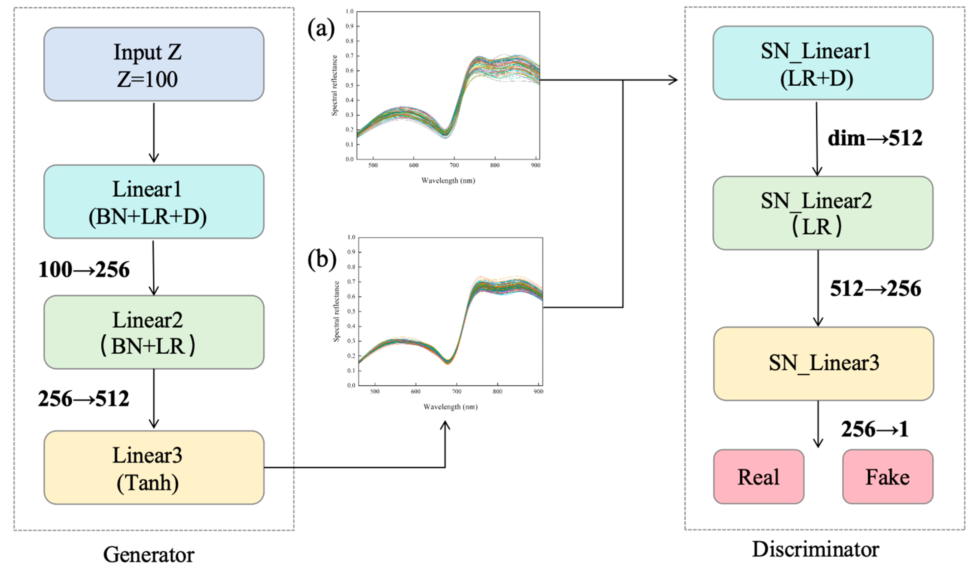
Regarding the design of the generator and discriminator, this study uses a multilayer perceptron (MLP) structure, stacking linear transformations, batch normalization, and LeakyReLU activation functions layer by layer. Additionally, a dropout mechanism is introduced in the middle layers to randomly discard hidden layers, enhancing feature representation and training stability. As shown in Figure 3, the generator takes a Gaussian random noise with a dimension of 100 as input and outputs a continuous spectral value sequence consistent with the spectral dimensions. The final layer uses a Tanh activation function to constrain the output within the [−1, 1] range, facilitating subsequent inverse normalization. The discriminator incorporates SpectralNorm constraints on the basic MLP architecture, regularizing each layer’s linear transformation to further enhance the network’s training stability and resistance to gradient explosion. The Sigmoid activation function is removed from the final layer to align with the Wasserstein distance metric.
During the training process, the model adopts the WGAN-GP loss structure and introduces a gradient penalty term to approximate the Lipschitz continuity condition, effectively alleviating issues of mode collapse and training instability commonly encountered in traditional GANs [27]. The discriminator is updated multiple times per round, and the Adam optimizer is used to improve model convergence efficiency. To further enhance the continuity and physical plausibility of the generated spectra, this study introduces a sliding average smoothing process for the generated samples, followed by inverse normalization and slight perturbation enhancement to improve the naturalness and distribution diversity of the spectral curves [28].

2.6.3. Early Detection Model

This study utilizes full-spectrum raw and augmented data, integrating multispectral fluorescence and reflectance from tomato plants, to train four machine learning models: RF, 1D-CNN, NB, and DT, in order to construct an early detection model for tomato gray mold.
Random Forest (RF) is an ensemble learning-based classification method that enhances precision and generalization through bootstrap sampling of multiple decision trees and a majority voting mechanism. It reduces overfitting risk by using random subsets of features [29]. One-Dimensional Convolutional Neural Network (1D-CNN) is a deep learning model specialized in processing one-dimensional sequences such as spectra. It automatically extracts features through convolutional layers, optimizes training by combining ReLU activation functions, batch normalization (BN) layers, and pooling layers, and outputs softmax classification results through fully connected layers [30]. Naive Bayes (NB) is a probabilistic model based on Bayes’ theorem and the assumption of feature independence, classifying by calculating posterior probabilities. It is characterized by a simple structure and high computational efficiency [31]. Decision Tree (DT) is a tree-structured classification model that recursively selects the optimal feature (based on the information gain criterion) to split nodes, generating highly interpretable classification rules [32].

2.6.4. Model Evaluation Method

The WGAN-GP model was validated using TSNE visualization, Frechet Inception Distance (FID), and Jensen–Shannon (JS) divergence. TSNE is a nonlinear dimensionality reduction technique designed to project high-dimensional data into two-dimensional space while preserving local similarities [33]. Although effective in revealing clustering patterns, it does not provide an exact representation of the true data manifold. When generated data and real data are closely intermixed in the TSNE plot, this indicates good generative performance, whereas a clear separation suggests poor generation quality. FID is a metric used to quantify distributional differences by comparing the means and covariance matrices of two datasets in a high-dimensional feature space; a smaller FID value indicates that the generated data are more similar to the real data [34]. JS divergence, derived from information theory, measures the similarity between two probability distributions, with smaller values indicating closer alignment. These metrics collectively were used to verify the reliability of data augmentation achieved by the WGAN-GP model [35].
For the PLSR model used for predicting physiological and biochemical indicators, the correlation coefficient of the prediction set (Rp2) and the root mean square error of prediction (RMSEP) were employed as evaluation metrics. Values of Rp2 closer to 1 and smaller RMSEP values indicate better predictive performance of the model.
R 2 = 1 i = 1 n y i y ^ i 2 i = 1 n y i y ¯ 2
R M S E = 1 n i = 1 n y i y ^ i 2
The actual observation value of the i-th observation is denoted as y i , the predicted value of the i-th observation is denoted as y ^ i , and the mean of the actual observation values is denoted as y ¯ .
In evaluating the detection model, precision is used as the main index to measure the proportion of samples that are predicted to be positive by the model. In addition to precision, it is also analyzed by F1 score and receiver operating characteristic curve (ROC). Precision predicts the proportion of correct classification for each category, and F1 score is used to evaluate the performance of classification model. ROC characteristic curve can evaluate and compare the comprehensive performance of different models. These metrics are derived from the confusion matrix, which provides a detailed explanation of the consistency between the actual and predicted categories, as defined by the formulas [36].
P r e c i s i o n = T P T P + F P
R e c a l l = T P T P + F N
F 1 = 2 P r e c i s i o n R e c a l l P r e c i s i o n + R e c a l l
In this context, TP (True Positive) represents the number of correct predictions for the positive class, TN (True Negative) represents the number of correct predictions for the negative class, FP (False Positive) represents the number of incorrect predictions classified as the positive class, and FN (False Negative) represents the number of incorrect predictions classified as the negative class.

2.7. Statistical Analysis

The t-test is a statistical method used to test the significance of differences between the means of two groups of data, thus assessing the influence of different groups on the research results [37]. In this study, the t-test was used to compare the differences in physiological and multispectral indicators between healthy tomatoes and tomatoes infected with gray mold. After identifying significant differences (p < 0.05), further analysis of the specific differences between the two groups was conducted. Pearson correlation analysis is a statistical method used to measure the degree of linear correlation between two variables, thus assessing the relationship between the variables [38]. In this study, a correlation heatmap was generated to visually represent the relationship between the physiological characteristics and multispectral indicators of gray mold-infected tomatoes.

3. Results and Analysis

3.1. Effects of Botrytis cinerea Infection on Tomato Physiological Characteristics

The physiological changes in plants following Botrytis cinerea infection help elucidate the tomato’s response to pathogen infection. In this study, photosynthetic pigment content, relative water content (WC), MDA content, and the activities of antioxidant enzymes (SOD and CAT) were measured to represent the biological response of tomatoes to gray mold.
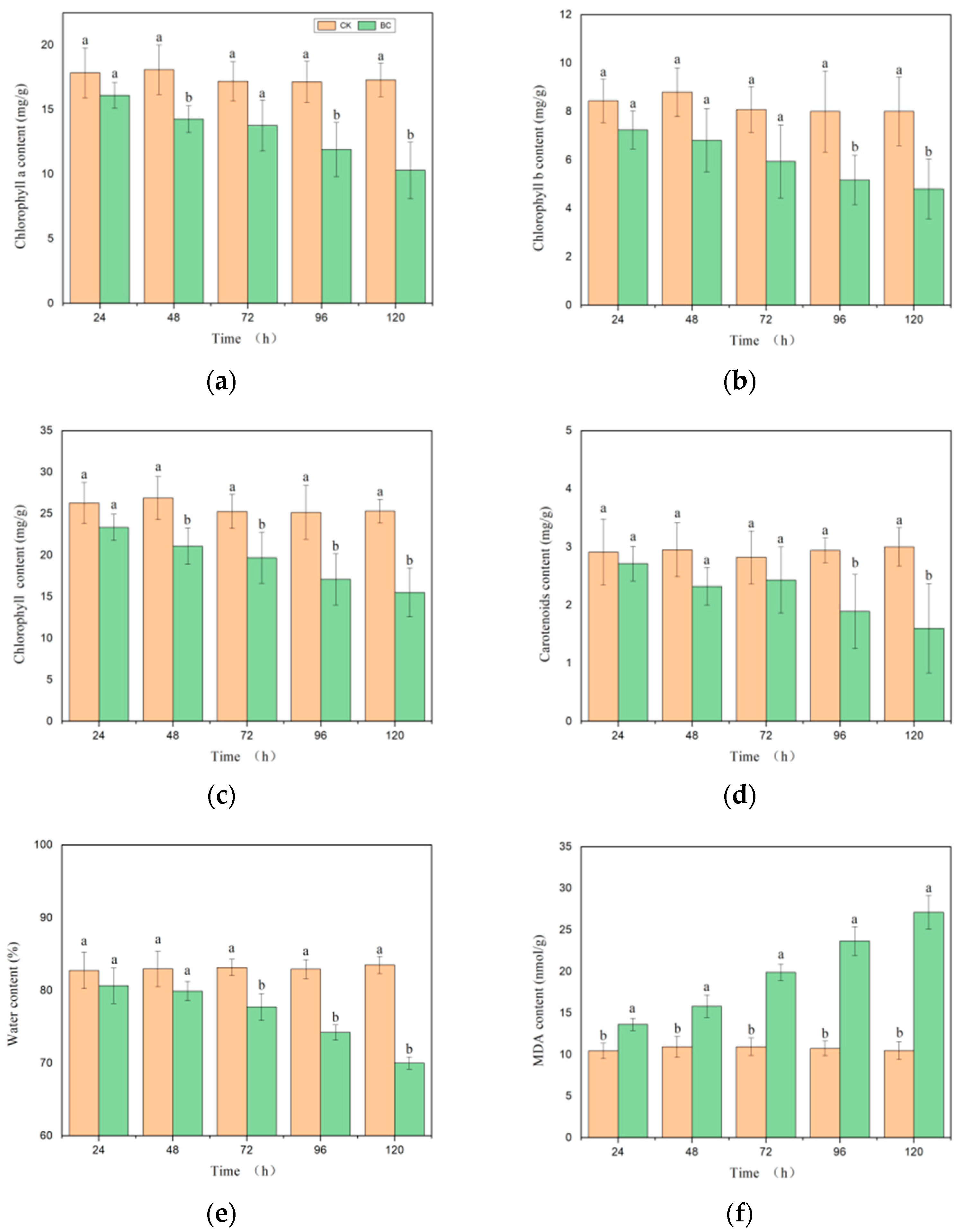
As shown in Figure 4, compared to the control group (CK), the BC group exhibited a time-dependent decrease in the contents of total chlorophyll (TCHL), chlorophyll a (CHLa), chlorophyll b (CHLb), carotenoids (CAR), and water content (WC) (p < 0.05). The MDA content in the BC group was increased by 164.7% at 120 h compared to the CK group (p < 0.01). The water content (WC) declined continuously from 24 h, with a total reduction of 13.2% (p < 0.01). The activities of the antioxidant enzymes CAT and SOD showed an initial increase followed by a subsequent decrease.

3.2. Effects of Botrytis cinerea Infection on Tomato Biochemical Characteristics

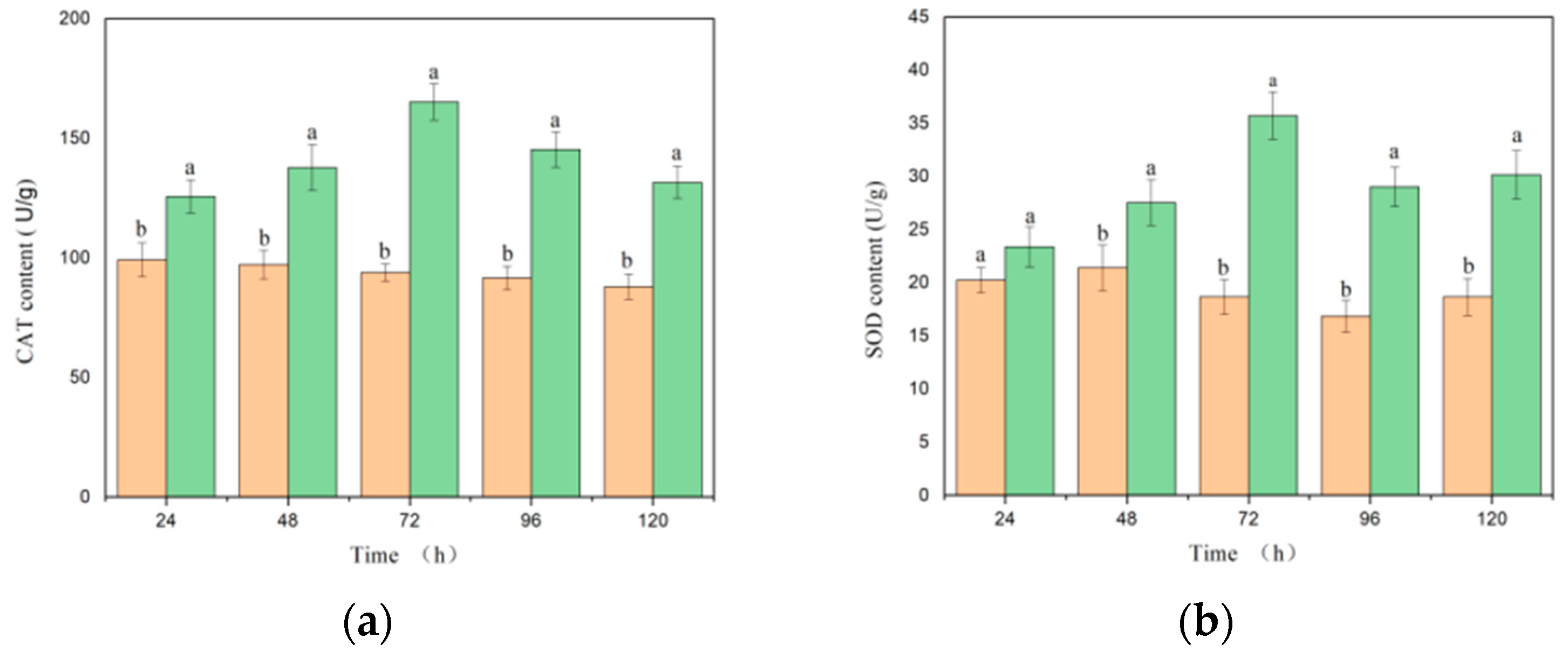
Following infection by Botrytis cinerea, the activities of superoxide dismutase (SOD) and catalase (CAT) in tomato leaves were significantly activated, exhibiting a highly consistent dynamic trend. As shown in Figure 5, compared with their respective control groups, the inoculated treatment group (BC) displayed a markedly higher activity of both SOD and CAT at all measured time points (p < 0.05). The temporal changes in the two enzymes were highly synchronized, with both reaching peak activity at 72 h post-inoculation. At this point, SOD activity was 1.9 times that of the control group, while CAT activity was 1.76 times higher. Thereafter, the activities of both enzymes declined from their peaks but remained significantly above control levels even at 120 h post-inoculation.

3.3. Response of Tomato Leaves to Multispectral Reflectance Under Botrytis cinerea Infection

3.3.1. Multispectral Reflectance and Vegetation Index Analysis of Tomato Leaves

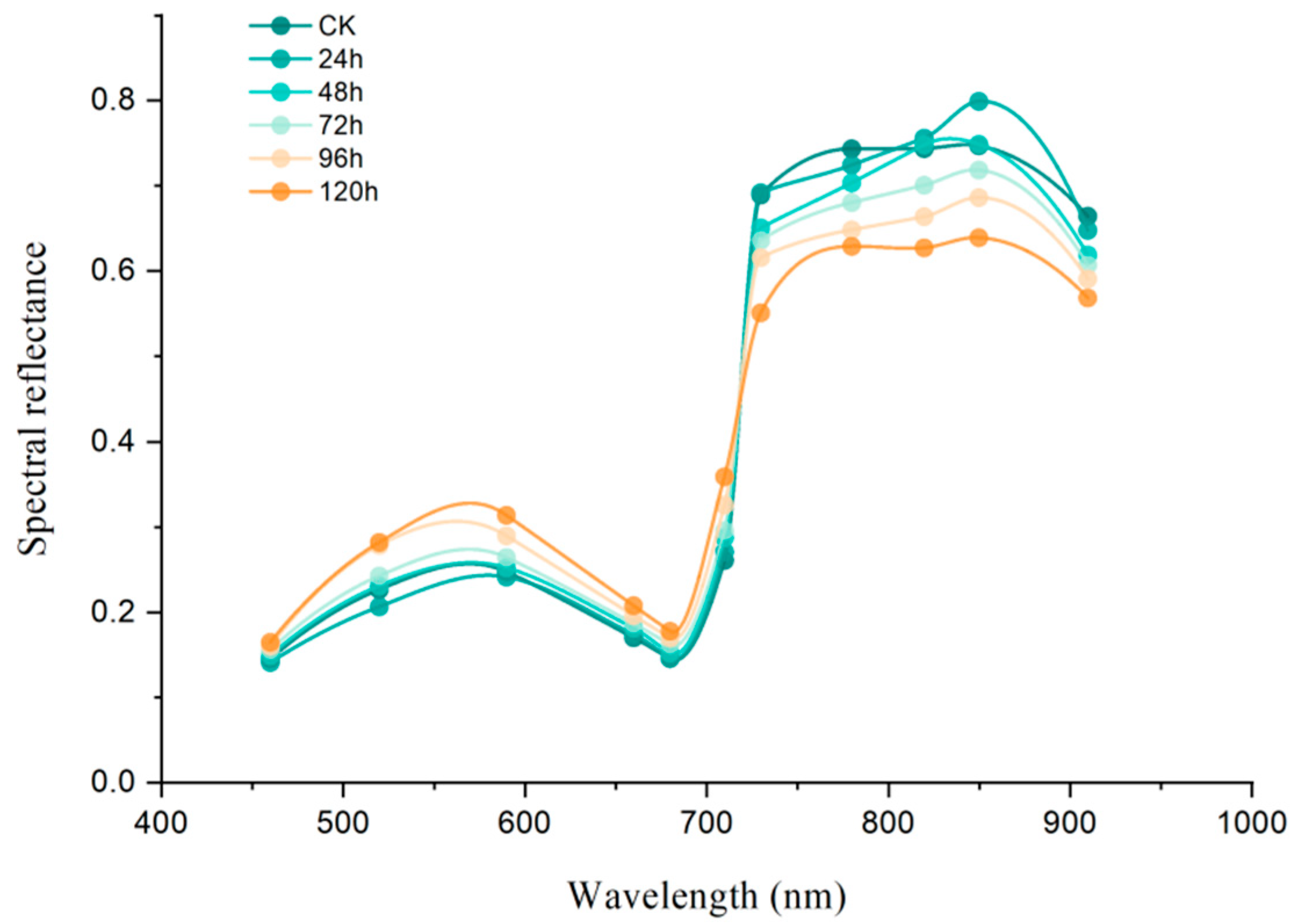
The spectral reflectance characteristics of tomato leaves provide key quantitative information for non-destructive and indirect evaluation of plant physiological status. Figure 6 shows the average spectral reflectance of CK and 24 h, 48 h, 72 h, 96 h, and 120 h after inoculation. According to Figure 5, after Botrytis cinerea infection, the reflectance of tomato leaves showed a dynamic process of first increasing near 700 nm and then decreasing over time at higher wavelengths. The absorption peaks or valleys in the spectral curves reflect changes in the spectrum, effectively capturing the dynamic changes in the plant’s physiological state and internal structure after tomato infection. The curves indicate that the reflectance in the visible light region is significantly lower than that in the near-infrared region for all samples. Compared to the CK group, the reflectance values of the BC group generally increased over time in the visible and red-edge regions. This suggests that the absorption of visible light by the leaves decreases, which may be related to chlorophyll degradation. Reflectance in the near-infrared region shows a general downward trend over time. The near-infrared reflectance is associated with the internal structure and water content of the leaves; a decrease may indicate leaf structural deterioration, water loss, or increased intercellular space.
By integrating information from multiple spectral bands, vegetation indices provide a more comprehensive reflection of plant physiological status, while effectively reducing incidental fluctuations or measurement errors that may occur in single-band data, thereby improving stability and reliability. Accordingly, five representative vegetation indices were selected for analysis in this study. As shown in Table 1, NDVI, GNDVI, and OSAVI exhibited a continuous decline during 0–96 h of infection (L1–L4), whereas the WI increased monotonically, indicating enhanced water uptake (potentially followed by water loss at later stages). PRI, on the other hand, displayed fluctuating changes. Notably, after 120 h of infection (L5 stage), NDVI and GNDVI showed a marked rebound, returning to or even exceeding their initial levels. This nonlinear spectral rebound is intriguing and may reflect profound alterations in plant tissue structure and physiological state during late-stage disease progression: (1) Tissue necrosis and desiccation: Severe infection leads to cellular necrosis, collapse, and dehydration. Rapid chlorophyll degradation reduces red light absorption (increasing red reflectance), while desiccated necrotic tissue markedly enhances near-infrared scattering (increasing near-infrared reflectance). The combined effect of these processes may explain the index rebound. (2) Potential late-stage physiological responses: such as changes in pigment composition or the accumulation of secondary metabolites. This phenomenon suggests that relying solely on NDVI or GNDVI for gray mold detection may lead to misclassification. Instead, a multi-index approach incorporating indicators of water status (WI) and photochemical efficiency (PRI) should be adopted for comprehensive assessment. Furthermore, the “decline–rebound” pattern observed here may serve as a distinguishing feature of gray mold, setting it apart from other stresses that typically manifest as a continuous decline in vegetation indices.

3.3.2. Changes in Multispectral Fluorescence of Tomato Leaves Under Gray Mold Infection

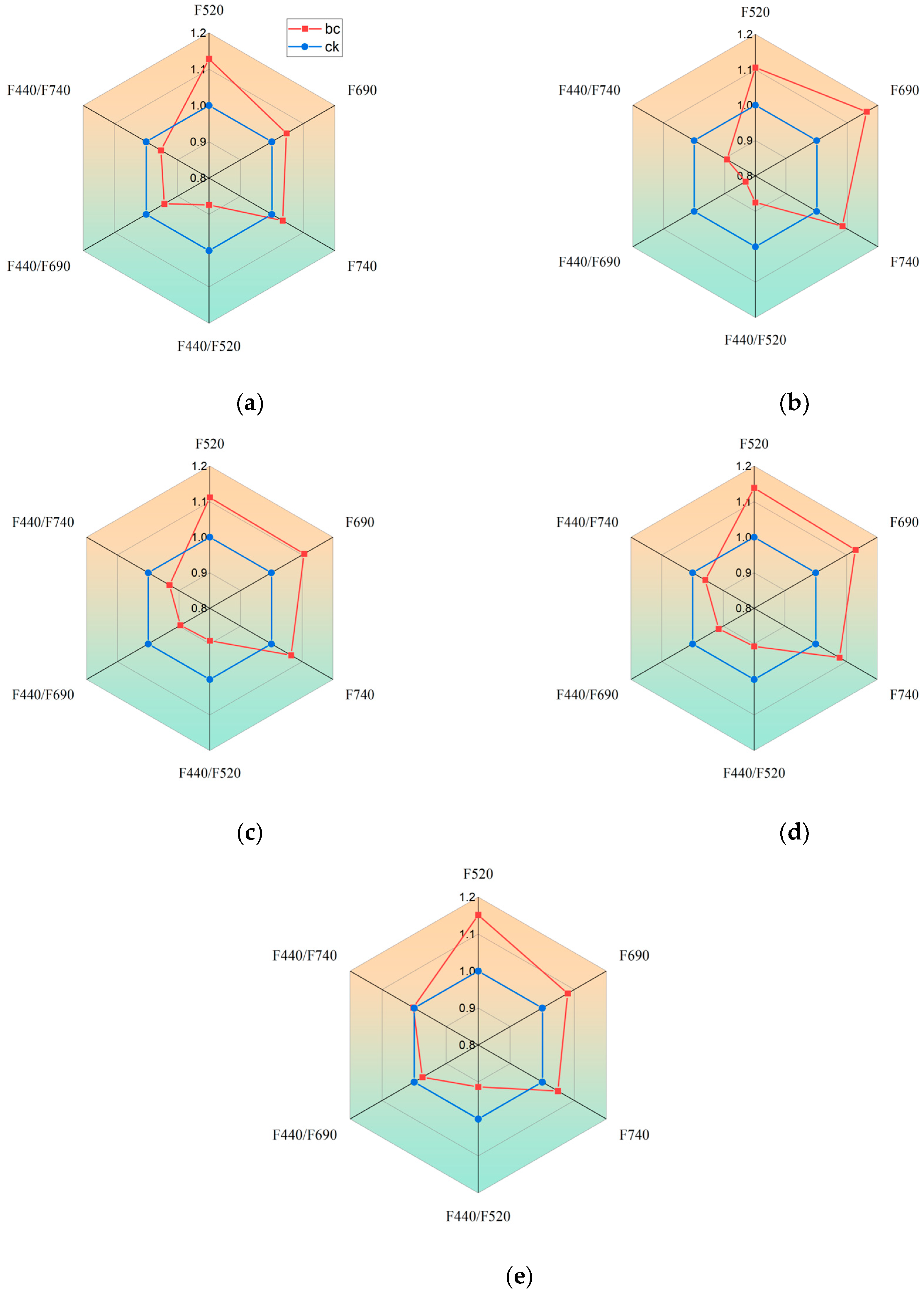
Following infection of tomato plants by Botrytis cinerea, the fluorescence ratio parameters exhibited regular variations in line with disease progression, reflecting the dynamic physiological responses of the plants. In this study, fluorescence bands (F520, F690, F740) and ratio parameters (F440/F520, F440/F690, F440/F740) showing significant differences between the experimental and control groups were selected for detailed analysis.
As shown in Figure 7, the single bands F520, F690, and F740 all increased after inoculation, peaking at 48 h before gradually declining. Among the ratio parameters, F440/F520 continuously increased from 24 h to 120 h, indicating a relative enhancement of F440 during this period. In contrast, F440/F690 and F440/F740 both decreased to their lowest values at 48 h, followed by a gradual recovery.
These consistent patterns suggest that 48 h post-inoculation represents a critical phase of pronounced photosynthetic system response, likely corresponding to the rapid disease development stage of gray mold. The dynamic changes across parameters revealed both the inhibition of photochemical activity and the activation of self-regulation mechanisms during infection, confirming that the selected fluorescence bands and ratios hold strong potential for early detection of gray mold in tomato plants.

3.4. Augmentation of Tomato Gray Mold Spectra Using the WGAN-GP Generative Adversarial Network

Using the WGAN-GP generative adversarial network, the original spectral data of tomato gray mold were augmented. Both the generator and discriminator learning rates were set to 0.0001, with a batch size of 32 and 500 training epochs. As a result, the number of samples per disease severity level was expanded to 260.
To verify the reliability of the proposed data augmentation method, generated and real data were compared and evaluated from multiple perspectives. As shown in Figure 8, TSNE dimensionality reduction was applied to visualize data at the L4 level, where the close intermixing of generated and real data indicated good generative performance. In Table 2, the FID scores for all severity levels were below 1, suggesting negligible differences between generated and real distributions. The JS divergence values, which range from 0 to 1, were closer to 0, indicating high similarity between the two distributions in probability space. Collectively, these results validated the reliability of the augmented data and confirmed the effectiveness of the model in feature extraction and high-quality sample generation.

3.5. PLSR Predictive Model for Physiological and Biochemical Indicators

To explore the predictive ability of multispectral parameters for the physiological and biochemical status of plants, this study developed a Partial Least Squares Regression (PLSR) model using the acquired spectral parameters (22 multispectral reflectance parameters, 10 multispectral fluorescence parameters, 5 SR indices) and 8 key physiological and biochemical indicators.
First, a comprehensive Pearson correlation analysis was conducted between all physiological and biochemical indicators and spectral parameters (Figure 9). The results indicate a strong correlation between physiological and biochemical indicators and spectral parameters, validating the potential of spectral data for predicting physiological states. Further analysis shows that the Pearson correlation coefficients among multispectral reflectance parameters vary widely (−0.50 to 0.97), while the correlation coefficients among fluorescence parameters show a narrower range (−0.42 to 0.95), with stronger internal correlations in the reflectance parameters. The correlation differences in the original fluorescence bands are significant, and there is a high positive correlation between fluorescence ratios, indicating information overlap. The correlation between reflectance and fluorescence parameters is lower than within each group, suggesting that they reflect different aspects of plant physiological status, and their combined use offers a more comprehensive assessment of plant physiological status.
Due to strong multicollinearity among the spectral parameters, the PLSR method was selected as it effectively handles correlations between independent variables. Through PLSR modeling and variable importance analysis, the most critical spectral wavelengths/indices for predicting each physiological and biochemical indicator were identified, and the model’s predictive performance was evaluated. The PLSR model based on feature parameters is shown in Table 3.
The optimal PLSR models for different physiological and biochemical indicators show significant differences in prediction accuracy (Rp2) and error (RMSEP). The model for predicting malondialdehyde (MDA) content performed the best, with an Rp2 of 0.82 and the lowest RMSEP (0.42). This model primarily relies on the reflectance at R730 and R710, as well as the green light normalized difference vegetation index (GNDVI) and photochemical reflectance index (PRI). The model for relative water content (RWC) also showed good predictive ability (R2 = 0.73, RMSEP = 0.47), with key variables focused on R730 and R710. Models for total chlorophyll (TCHL), catalase (CAT), and superoxide dismutase (SOD) activities showed relatively lower prediction accuracy (R2 values of 0.42, 0.25, and 0.32, respectively). The TCHL model primarily relies on reflectance (R730/R710/R460/R520 negative), while the CAT and SOD models combine fluorescence parameters (F520, F690/F740) and reflectance parameters (R850/R460/R730/GNDVI).

3.6. Model Comparison

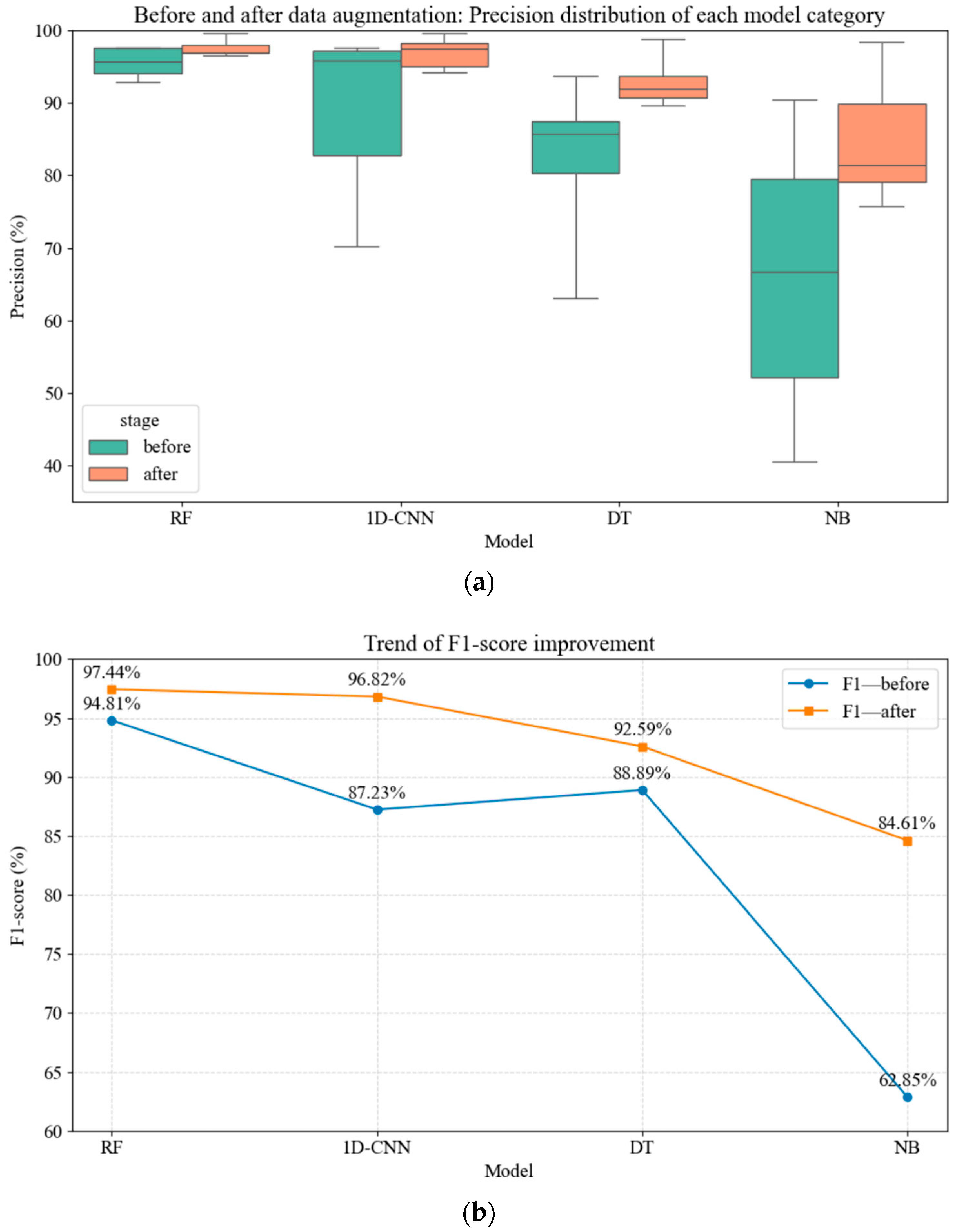
Based on the collected experimental data, we first classified the samples into different grades and then performed data augmentation separately. After applying perturbation-based enhancement to the entire dataset, an additional column was added to label the infection level. The augmented data were subsequently combined and used in model training with 10-fold cross-validation. A 10-fold cross-validation was used during model training. The training results from four machine learning models—RF, 1D-CNN, NB, and DT—are shown in the confusion matrix in Figure 10. After data augmentation, the performance of all models improved significantly. Among them, NB achieved the largest average precision improvement of 18.88%, while the precision for the weak classes L2 and L3 in 1D-CNN increased by more than 15%. Furthermore, as shown in the figure, the inter-class disparity was reduced in all models, and the volatility of 1D-CNN and NB decreased significantly.
As shown Figure 11, among all the models compared, the RF model demonstrated the best performance, achieving an overall classification precision of 97.56% for healthy plants and plants with different disease severity levels. Specifically, as shown in Table 4 and Table 5, it reached a precision of 96.92% for healthy plants, between 96.54% and 98.46% for early-stage diseased plants (L1–L4), and as high as 99.62% for L5-level diseased plants. It is worth noting that the model achieved precision values above 96.9% for L3–L5 severity levels, with an AUC value of 0.999 (Figure 12). The 1D-CNN model attained an overall precision of 96.92%, second only to the RF model. It achieved the highest precision of 97.31% for healthy plants and 97.69% for L1-level diseased plants. However, its precision for L2–L3 levels was only 94.23%, significantly lower than that of the RF model. The DT model achieved an overall accuracy of 92.82%, with the lowest precision for healthy plants at 89.62%. Its ability to classify L2–L5 diseased plants showed a gradient improvement, exceeding 94% precision for L4–L5 levels, but it performed worse than the RF model in distinguishing early-stage infections. The NB model had the lowest overall accuracy at 84.68%. It performed poorly in classifying L1–L4 diseased plants, with precision values ranging only from 75.77% to 81.54%, indicating insufficient capability in identifying early disease symptoms.
In this study, the Random Forest (RF) model was ultimately selected for the non-destructive early detection of tomato gray mold. To further investigate which key features guided the classification process, we evaluated the importance of each feature using the RF model. Feature importance was calculated based on the reduction in Gini impurity contributed by each feature. During training, every decision tree splits nodes according to specific features, and the importance score of a feature is obtained as the weighted average of its impurity reduction across all trees. This method not only captures the overall contribution of each feature but also accommodates nonlinear relationships and high-dimensional data. For intuitive interpretation, the importance scores of all features were ranked and visualized in a bar chart. In Figure 13, the length of each bar indicates how strongly the corresponding feature contributes to the classification task, while the black vertical line within each bar indicates the standard deviation of the feature importance across different trees, thereby reflecting the stability of the importance estimation. Such visualization not only reveals the relative contribution of features to the model’s predictions but also illustrates the uncertainty in importance estimation through standard deviations, providing a basis for subsequent feature selection and model optimization.

4. Discussion

This study focused on the miniature tomato cultivar Micro-Tom to systematically evaluate the spectral responses of multispectral reflectance and chlorophyll fluorescence during the early stages of gray mold infection, and subsequently developed a high-accuracy disease recognition model. The experimental results, as shown in Figure 6, indicate that, after inoculation, reflectance at 460 nm and 520 nm in the visible range increased synchronously, while reflectance at 850 nm in the near-infrared region significantly decreased. The former corresponded to chlorophyll and carotenoid degradation, whereas the latter showed a strong negative correlation with MDA accumulation, thereby revealing spectroscopic signatures of internal structural damage and lipid peroxidation in leaf tissues.
With regard to multispectral fluorescence, the ratio F440/F690 exhibited a sharp change within 48 h post-inoculation, preceding the appearance of visible lesions. It declined to a minimum during the L1–L2 stages, suggesting that this parameter can capture a critical turning point in the interplay between pathogen spread and host defense. The low correlation between reflectance and fluorescence parameters further indicated that they represent different dimensions of plant physiology, namely structural integrity, pigment composition, and photosystem functionality. Their combined use thus provides a more comprehensive physiological assessment.
The PLSR-based quantitative inversion model yielded the highest predictive accuracy for MDA, with variables such as R730, R710 (reflectance), and F520, F690/F740 (fluorescence) playing central roles in explaining distinct physiological processes, highlighting their value as key parameters for early non-destructive detection. The RF algorithm achieved 96.54% recognition accuracy at 24 h and increased to 99.62% at 120 h, with an overall AUC of 0.999 and an F1 score of 0.974, demonstrating both effectiveness and robustness in early-stage detection. Compared with conventional destructive sampling and biochemical assays, this detection method enables rapid and non-invasive acquisition of physiological information. A single scan simultaneously captures both reflectance and fluorescence spectra, allowing synchronous estimation of multiple parameters such as MDA content and pigment degradation, thereby replacing numerous labor-intensive experimental steps and significantly improving detection efficiency.
Nevertheless, several limitations remain. First, the miniature cultivar Micro-Tom differs from common commercial cultivars in plant architecture, leaf morphology, and physiological traits, which may lead to variations in spectral responses and disease progression patterns. Therefore, cross-varietal validation and appropriate model calibration or retraining are required before practical application to other cultivars. Second, model training and validation were conducted under controlled environmental conditions, which, although suitable for proof-of-concept testing, do not fully reflect the complexities of field environments, including variable illumination, heterogeneous backgrounds, and the coexistence of multiple biotic and abiotic stresses. The robustness of the model in real agricultural scenarios, therefore, requires further evaluation. Third, it is important to acknowledge the limitations of this study. Although data augmentation strategies were employed to expand the sample size, the scale of the original, authentic dataset remained relatively limited. Moreover, it should be noted that the erroneous application of data augmentation across all datasets may have led to overly optimistic performance evaluations. These factors likely constrained the model’s ability to fully capture phenotypic diversity and generalize across varying conditions. Future studies should therefore prioritize the use of larger-scale, multi-source datasets and adhere to more rigorous data partitioning protocols to enhance the reliability and adaptability of the model [39].
Future research will expand in several directions. (1) Broadening the range of crop cultivars studied and integrating data from diverse varieties and advanced algorithms to enhance model generalization; conducting field trials across different regions and environments to improve adaptability and robustness. (2) Incorporating explainable XAI techniques to develop hybrid models that enhance interpretability [40], while constructing multitask learning frameworks capable of simultaneously detecting gray mold and other crop stresses. (3) Further optimizing early detection capabilities by integrating predictive algorithms for proactive disease prevention, shifting plant health management from reactive control to proactive prevention. (4) Developing lightweight models for integration into robotic platforms and unmanned aerial vehicles (UAVs), enabling large-scale automated monitoring and advancing the level of intelligent agriculture [41,42].

5. Conclusions

Both multispectral fluorescence and reflectance are responsive to the progression of tomato gray mold, and their combined application enables earlier and more accurate detection of the disease. This study explored an early detection method for Botrytis cinerea in tomatoes by integrating multispectral fluorescence-reflectance imaging with machine learning. The conclusions are as follows:
(1)
The synergistic integration of fluorescence and reflectance imaging can sensitively capture early physiological damage, and their complementarity markedly enhances the sensitivity of disease detection at the initial stage.
(2)
The development of the disease stages in tomatoes is mainly related to changes in malondialdehyde (MDA) and water content, and there is a certain correlation with changes in chlorophyll, superoxide dismutase (SOD), and catalase (CAT) levels. Physiological and biochemical indicators show strong correlations with all spectral parameters.
(3)
The Random Forest (RF) model with data augmentation achieved the best performance, with an average accuracy of 97.56% and an F1 score of 97.44%. Its overall recognition rate for early-stage diseased plants (L1–L4) reached 97.21%, significantly outperforming the 1D-CNN, DT, and NB models.
(4)
Data augmentation significantly enhanced the generalization ability of all models. Specifically, the NB model exhibited an 18.88% improvement in average accuracy, while the 1D-CNN achieved over 15% higher recognition rates for weaker classes (L2/L3). In addition, inter-class performance disparities among models were reduced, and the variability (standard deviation) of both RF and 1D-CNN decreased by more than 40%.
In summary, the integration of multispectral fluorescence and reflectance, by capturing early physiological damage in tomatoes, combined with data-augmented RF models, achieves a 97.21% disease identification rate for early-stage disease levels (L1–L4), providing reliable technical support for precise early warning of Botrytis cinerea in tomatoes.

Author Contributions

Conceptualization, X.Z., H.L., Y.C., Y.D., H.X. and J.T.; Data curation, X.Z., H.L. and M.R.; Formal analysis, X.Z., H.L., J.T., S.L., M.H., L.W. and C.Z.; Funding acquisition, F.Z. and L.X.; Investigation, X.Z., H.L., Y.C., Y.D., H.X., J.T., L.W. and H.W.; Methodology, X.Z., Y.C., Y.D., H.X., J.T., L.W., S.L. and L.X.; Project administration, X.Z., H.L., J.T., M.H., H.W., M.R., F.Z. and L.X.; Resources, F.Z. and S.L.; Software, X.Z., H.L., Y.C., Y.D., H.X. and C.Z.; Supervision, F.Z. and L.X.; Validation, X.Z., H.L., Y.C., Y.D., M.H., H.W., M.R., L.W. and C.Z.; Visualization, H.L. and Y.C.; Writing—original draft, X.Z., H.L., Y.C., H.X., S.L. and H.W.; Writing—review and editing, X.Z., H.L., Y.D., M.H., M.R., F.Z. and L.X. All authors have read and agreed to the published version of the manuscript.

Funding

This research was funded by the following grants: Facility Solanaceous Vegetable Breeding and Industrialization Development Sub-topics (2023Fjnk04009); Seed Industry Innovation and Industrialization Project in Fujian Province (zycxny2021009); Fujian Modern Agricultural Vegetable Industry System Construction Project (2019-897).

Data Availability Statement

Since the project presented in this research has not yet concluded, the experimental data will not be disclosed for the time being. If the reader requires any additional information. The first author will provide the requested information.

Acknowledgments

We sincerely thank our fellow students who provided support and assistance during the experiments. We thank all the good teachers and beneficial friends who have cared for, supported, and helped out. Lastly, we heartily thank all the experts who took time out of their busy schedules to review this paper and offer their valuable suggestions.

Conflicts of Interest

The authors declare no conflicts of interest.

References

  1. Ambresh, L.; Lingaiah, H.B.; Renuka, M.; Bhat, B.A. Development and characterization of recombinant inbreed lines for segregating bacterial wilt disease in tomato. Int. J. Curr. Microbiol. Appl. Sci. 2017, 6, 1050–1054. [Google Scholar] [CrossRef]
  2. Dean, R.; van Kan, J.A.L.; Pretorius, Z.A.; Hammond-Kosack, K.E.; Di Pietro, A.; Spanu, P.D.; Rudd, J.J.; Dickman, M.; Kahmann, R.; Ellis, J.; et al. The top 10 fungal pathogens in molecular plant pathology. Mol. Plant Pathol. 2012, 13, 414–430. [Google Scholar] [CrossRef]
  3. Sánchez-Sánchez, M.; Aispuro-Hernández, E.; Quintana-Obregón, E.A.; Vargas-Arispuro, I.C.; Martínez-Téllez, M.Á. Estimating tomato production losses due to plant viruses, a look at the past and new challenges. Comun. Sci. 2024, 15, e4247. [Google Scholar] [CrossRef]
  4. Singh, R.; Caseys, C.; Kliebenstein, D.J. Genetic and molecular landscapes of the generalist phytopathogen Botrytis cinerea. Mol. Plant Pathol. 2024, 25, e13404. [Google Scholar] [CrossRef] [PubMed]
  5. Hahn, M. The rising threat of fungicide resistance in plant pathogenic fungi: Botrytis as a case study. J. Chem. Biol. 2014, 7, 133–141. [Google Scholar] [CrossRef] [PubMed]
  6. Asselbergh, B.; Curvers, K.; França, S.C.; Audenaert, K.; Vuylsteke, M.; Van Breusegem, F.; Höfte, M. Resistance to Botrytis cinerea in sitiens, an abscisic acid-deficient tomato mutant, involves timely production of hydrogen peroxide and cell wall modifications in the epidermis. Plant Physiol. 2007, 144, 1863–1877. [Google Scholar] [CrossRef]
  7. Moter, A.; Göbel, U.B. Fluorescence in situ hybridization (FISH) for direct visualization of microorganisms. J. Microbiol. Methods 2000, 41, 85–112. [Google Scholar] [CrossRef]
  8. Liu, S.; Xu, H.; Deng, Y.; Cai, Y.; Wu, Y.; Zhong, X.; Zheng, J.; Lin, Z.; Ruan, M.; Chen, J.; et al. YOLOv8-LSW: A Lightweight Bitter Melon Leaf Disease Detection Model. Agriculture 2025, 15, 1281. [Google Scholar] [CrossRef]
  9. De Silva, M.; Brown, D. Multispectral plant disease detection with vision transformer–convolutional neural network hybrid approaches. Sensors 2023, 23, 8531. [Google Scholar] [CrossRef]
  10. Duan, Z.; Li, H.; Li, C.; Zhang, J.; Zhang, D.; Fan, X.; Chen, X. A CNN model for early detection of pepper Phytophthora blight using multispectral imaging, integrating spectral and textural information. Plant Methods 2024, 20, 115. [Google Scholar] [CrossRef]
  11. Guo, Z.; Sun, X.; Qin, L.; Dong, L.; Xiong, L.; Xie, F.; Qin, D.; Chen, Y. Identification of Golovinomyces artemisiae causing powdery mildew, changes in chlorophyll fluorescence parameters, and antioxidant levels in Artemisia selengensis. Front. Plant Sci. 2022, 13, 876050. [Google Scholar] [CrossRef]
  12. Matorin, D.N.; Timofeev, N.P.; Glinushkin, A.P.; Bratkovskaja, L.B.; Zayadan, B.K. Effect of fungal infection with Bipolaris sorokiniana on photosynthetic light reactions in wheat analyzed by fluorescence spectroscopy. Mosc. Univ. Biol. Sci. Bull. 2018, 73, 203–208. [Google Scholar] [CrossRef]
  13. Sapoukhina, N.; Boureau, T.; Rousseau, D. Plant disease symptom segmentation in chlorophyll fluorescence imaging with a synthetic dataset. Front. Plant Sci. 2022, 13, 969205. [Google Scholar] [CrossRef] [PubMed]
  14. Qiu, X.; Chen, H.; Huang, P.; Zhong, D.; Guo, T.; Pu, C.; Li, Z.; Liu, Y.; Chen, J.; Wang, S. Detection of citrus diseases in complex backgrounds based on image–text multimodal fusion and knowledge assistance. Front. Plant Sci. 2023, 14, 1280365. [Google Scholar] [CrossRef]
  15. Chen, Y.; Pan, J.; Wu, Q. Apple leaf disease identification via improved CycleGAN and convolutional neural network. Soft Comput. 2022, 27, 9773–9786. [Google Scholar] [CrossRef]
  16. Kanda, P.S.; Xia, K.; Sanusi, O.H. A deep learning-based recognition technique for plant leaf classification. IEEE Access 2021, 9, 162590–162613. [Google Scholar] [CrossRef]
  17. Min, B.; Kim, T.; Shin, D.; Shin, D. Data augmentation method for plant leaf disease recognition. Appl. Sci. 2023, 13, 1465. [Google Scholar] [CrossRef]
  18. Li, J.; Zeng, H.; Huang, C.; Wu, L.; Ma, J.; Zhou, B.; Ye, D.; Weng, H. Noninvasive detection of salt stress in cotton seedlings by combining multicolor fluorescence–multispectral reflectance imaging with efficientnet-OB2. Plant Phenomics 2023, 5, 0125. [Google Scholar] [CrossRef]
  19. Xu, F. Indirect photometric determination of chlorophyll in plant leaves. Phys. Test. Chem. Anal. B 2005, 41, 661–662. [Google Scholar] [CrossRef]
  20. Wang, J.-H.; Huang, W.-J.; Zhao, C.-J.; Yang, M.-H.; Wang, Z.-J. The inversion of leaf biochemical components and grain quality indicators of winter wheat with spectral reflectance. J. Remote Sens. 2003, 7, 277–284. [Google Scholar] [CrossRef]
  21. Senthilkumar, M.; Amaresan, N.; Sankaranarayanan, A. Estimation of malondialdehyde (MDA) by thiobarbituric acid (TBA) assay. In Plant-Microbe Interactions: Laboratory Techniques; Springer Science+Business Media: New York, NY, USA, 2021; pp. 103–104. [Google Scholar] [CrossRef]
  22. Li, C.; Kang, J.H.; Jung, K.I.; Park, M.H.; Kim, M. Effects of Haskap (Lonicera caerulea L.) extracts against oxidative stress and inflammation in RAW 264.7 cells. Prev. Nutr. Food Sci. 2024, 29, 146–153. [Google Scholar] [CrossRef]
  23. Zou, P.; Lu, X.; Jing, C.; Yuan, Y.; Lu, Y.; Zhang, C.; Meng, L.; Zhao, H.; Li, Y. Low-molecular-weight polysaccharides from Pyropia yezoensis enhance tolerance of wheat seedlings (Triticum aestivum L.) to salt stress. Front. Plant Sci. 2018, 9, 427. [Google Scholar] [CrossRef] [PubMed]
  24. Xie, C.; Yang, C.; He, Y. Hyperspectral Imaging for Classification of Healthy and Gray Mold Diseased Tomato Leaves with Different Infection Severities. Comput. Electron. Agric. 2017, 135, 154–162. [Google Scholar] [CrossRef]
  25. Wang, X.Q.; Chen, S.Y.; Zheng, W.C. Traffic Incident Duration Prediction Based on Partial Least Squares Regression. Procedia Soc. Behav. Sci. 2013, 96, 425–432. [Google Scholar] [CrossRef]
  26. Koumoutsou, D.; Siolas, G.; Charou, E.; Stamou, G. Generative Adversarial Networks for Data Augmentation in Hyperspectral Image Classification. In Generative Adversarial Learning: Architectures and Applications; Springer: Cham, Switzerland, 2022; pp. 115–136. [Google Scholar] [CrossRef]
  27. Li, Y.; Wang, B.; Yang, Z.; Li, J.; Chen, C. Hierarchical Stochastic Scheduling of Multi-Community Integrated Energy Systems in Uncertain Environments via Stackelberg Game. Energy Convers. Manag. 2022, 235, 113996. [Google Scholar] [CrossRef]
  28. Zhang, F.F.; Li, J.S.; Wang, C.; Wang, S.L. Estimation of water quality parameters of GF-1 WFV in turbid water based on soft classification. Natl. Remote Sens. Bull. 2023, 27, 769–779. [Google Scholar] [CrossRef]
  29. Breiman, L. Random forests. Mach. Learn. 2001, 45, 5–32. [Google Scholar] [CrossRef]
  30. Kiranyaz, S.; Avci, O.; Abdeljaber, O.; Ince, T.; Gabbouj, M.; Inman, D.J. 1D convolutional neural networks and applications: A survey. Mech. Syst. Signal Process. 2021, 151, 107398. [Google Scholar] [CrossRef]
  31. Zhang, Z.H. Naïve Bayes classification in R. Ann. Transl. Med. 2016, 4, 241. [Google Scholar] [CrossRef]
  32. Silva Júnior, A.C.; Moura, W.M.; Bhering, L.L.; Siqueira, M.J.S.; Costa, W.G.; Nascimento, M.; Cruz, C.D. Prediction and importance of predictors in approaches based on computational intelligence and machine learning. Agron. Sci. Biotechnol. 2023, 9, 1–24. [Google Scholar] [CrossRef]
  33. Arora, S.; Hu, W.; Kothari, P.K. An Analysis of the t-SNE Algorithm for Data Visualization. In Proceedings of the Conference on Learning Theory (COLT), Stockholm, Sweden, 6–9 July 2018; Volume 75, pp. 1–32. [Google Scholar]
  34. DeVries, T.; Taylor, G.W.; Romero, A.; Pineda, L.; Drozdzal, M. On the Evaluation of Conditional GANs. arXiv 2019, arXiv:1907.08175 2019. [Google Scholar] [CrossRef]
  35. Liu, Y.; Gao, Y.; Yue, L.; Zhang, H.; Sun, J.; Wu, X. A Real-Time Detection of Pilot Workload Using Low-Interference Devices. Appl. Sci. 2024, 14, 6521. [Google Scholar] [CrossRef]
  36. Muningsih, E. Kombinasi Metode K-Means dan Decision Tree dengan Perbandingan Kriteria dan Split Data. J. Teknonfo 2022, 16, 113–118. [Google Scholar] [CrossRef]
  37. Kim, T.K. T test as a parametric statistic. Korean J. Anesthesiol. 2015, 68, 540–546. [Google Scholar] [CrossRef]
  38. Franzese, M.; Iuliano, A. Correlation Analysis. Encycl. Bioinform. Comput. Biol. 2019, 1, 706–721. [Google Scholar] [CrossRef]
  39. Zhang, Z.; Ma, L.; Wei, C.; Yang, M.; Qin, S.; Lv, X.; Zhang, Z. Cotton Fusarium wilt diagnosis based on generative adversarial networks in small samples. Front. Plant Sci. 2023, 14, 1290774. [Google Scholar] [CrossRef]
  40. Cho, S.B.; Soleh, H.M.; Choi, J.W.; Hwang, W.-H.; Lee, H.; Cho, Y.-S.; Cho, B.-K.; Kim, M.S.; Baek, I.; Kim, G. Recent Methods for Evaluating Crop Water Stress Using AI Techniques: A Review. Sensors 2024, 24, 6313. [Google Scholar] [CrossRef] [PubMed]
  41. Liu, J.; Xiang, J.; Jin, Y.; Liu, R.; Yan, J.; Wang, L. Boost Precision Agriculture with Unmanned Aerial Vehicle Remote Sensing and Edge Intelligence: A Survey. Remote Sens. 2021, 13, 4387. [Google Scholar] [CrossRef]
  42. Popescu, D.; Stoican, F.; Stamatescu, G.; Ichim, L.; Dragana, C. Advanced UAV–WSN System for Intelligent Monitoring in Precision Agriculture. Sensors 2020, 20, 817. [Google Scholar] [CrossRef]
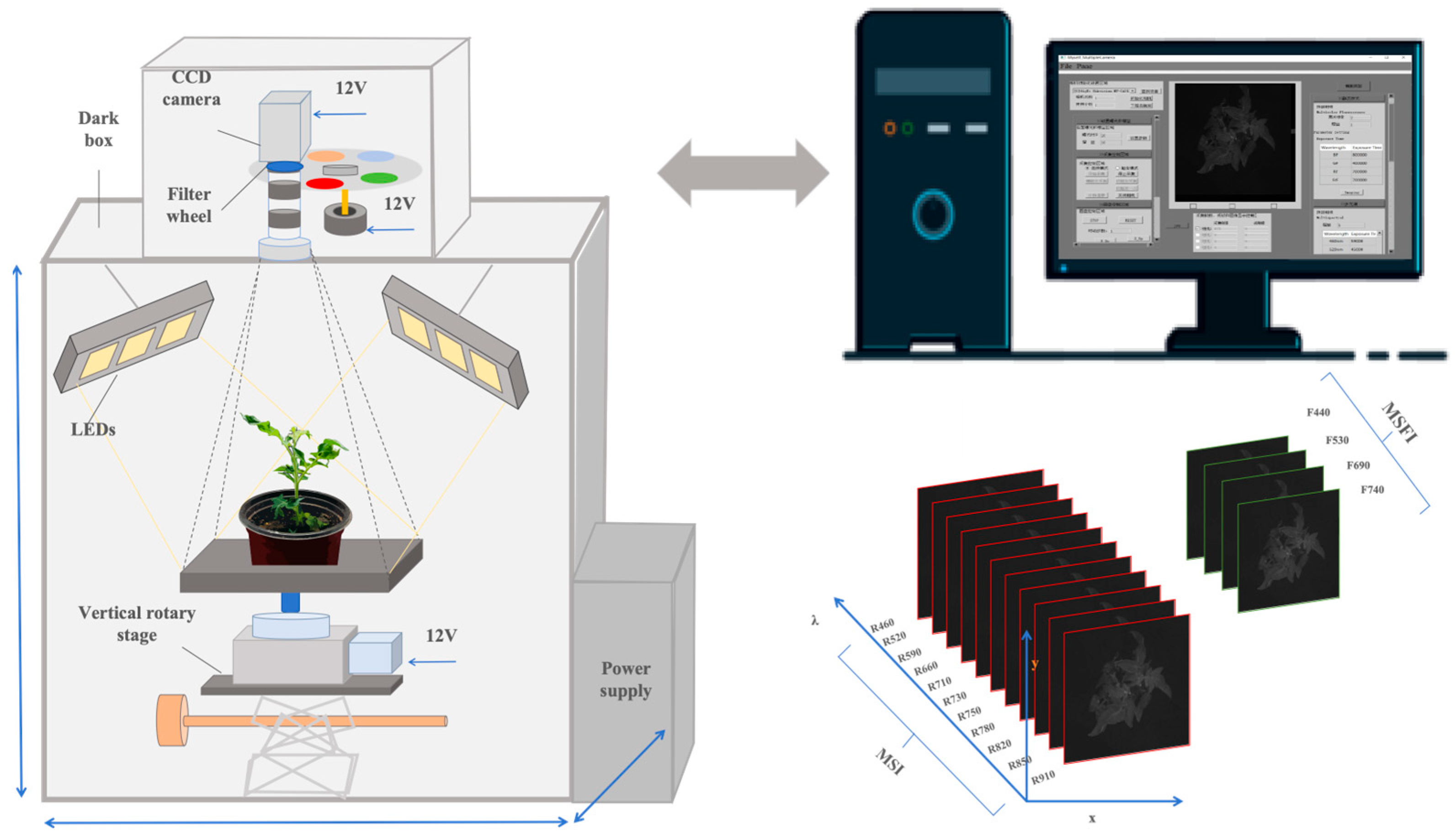
Figure 1. Schematic diagram of the multispectral data acquisition and analysis platform set. Note: MSI stands for Multispectral Imaging; MSFI stands for Multispectral Fluorescence Imaging.
Horticulturae 11 01073 g001
Figure 2. DCGAN Flowchart. Note: G stands for Generator; D stands for Discriminator; z stands for Latent random variable; x stands for Real data; D(x) stands for Discriminator’s output for real data; G(z) stands for Generated data; D(G(z)) stands for Discriminator’s output for generated data. Discrimination; Real/Fake stands for Real/Fake discrimination. The black circles represent adding random noise to the data, the green circles represent the discriminator’s judgment of the data as “real”, and the red circles represent the discriminator’s judgment of the data as “fake”.
Horticulturae 11 01073 g002
Figure 3. DCGAN network parameters. (a) Original reflectance curve graph; (b) Reflection curve graph of enhanced data. Note: BN stands for Batch Normalization; LR stands for LeakyReLU; D stands for Dropout; Tanh stands for Hyperbolic Tangent; SN stands for Spectral Normalization; Linear stands for Linear Layer; Real/Fake stands for Real/Fake discrimination.
Horticulturae 11 01073 g003
Figure 4. Changes in physiological characteristics of tomatoes under Botrytis cinerea infection. (a) Change in chlorophyll a content; (b) Change in chlorophyll b content; (c) Change in chlorophyll total content; (d) Change in carotenoid content; (e) Comparison of water content; (f) Comparison of MDA content. The lowercase letters in the figures indicate saliency at p < 0.05. The error line in the figure represents ± standard deviation (SD), n = 10.
Horticulturae 11 01073 g004
Figure 5. Changes in biochemical indicators of tomatoes under Botrytis cinerea infection. (a) Comparison of CAT content; (b) Comparison of SOD content. The lowercase letters in the figures indicate saliency at p < 0.05. The error line in the figure represents ± standard deviation (SD), n = 10.
Horticulturae 11 01073 g005
Figure 6. Curve of Changes in Average Reflectivity of Infected Tomatoes 24–120 h and CK.
Horticulturae 11 01073 g006
Figure 7. Multispectral fluorescence parameters of tomato leaves infected by Botrytis cinerea at L1-L5 (24–120 h). (a) L1; (b) L2; (c) L3; (d) L4; (e) L5.
Horticulturae 11 01073 g007
Figure 8. L4 TSNE Visualization of Real vs. Generated Data.
Horticulturae 11 01073 g008
Figure 9. Heat map of Pearson’s correlation coefficient between different parameters.
Horticulturae 11 01073 g009
Figure 10. (a) Before and after data augmentation: Precision distribution of each model category; (b) Trend of Fl-score improvement.
Horticulturae 11 01073 g010
Figure 11. (a) Confusion matrix based on original samples, (b) Confusion matrix based on data augmentation.
Horticulturae 11 01073 g011
Figure 12. ROC of the augmented model.
Horticulturae 11 01073 g012
Figure 13. Random Forest Feature importance.
Horticulturae 11 01073 g013
Table 1. Changes in vegetation indices under Botrytis cinerea infection.
TimeNDVIPRIWIGNDVIOSAVI
CK0.61−0.080.810.560.52
24 h0.59−0.040.830.510.50
48 h0.57−0.040.850.480.48
72 h0.54−0.020.860.400.45
96 h0.50−0.050.890.380.42
120 h0.64−0.090.850.590.54
Table 2. Validation metrics for data augmentation.
CategoryFID ScoreJS Divergence
C00.050.03
L10.080.04
L20.050.03
L30.050.02
L40.080.02
L50.030.02
Table 3. Model accuracy test.
CategoryIndicatorsEquationRp2RMSEP
PhysiologicalMDAMDA = −0.64*R730 + 0.91*R710 + 0.48*GNDVI + 0.21*PRI0.820.42
WCWC = +0.52*R730 − 0.65*R710 − 0.17*GNDVI − 0.08*R5900.730.47
TCHLTCHL = 0.44*R730 − 0.19*R710 − 0.17*R460 − 0.16*R5200.420.72
BiochemicalSODSOD = +0.34*F520 + 0.28*F690/F740 + 0.38*R460 − 0.22*R7300.320.40
CATCAT = +0.51*F520 + 0.25*F690/F740 + 0.27*R850 − 0.48*GNDVI0.250.76
Table 4. Classification precision of each model based on the original training set at different disease levels.
ModelsPrecision F1-Score
C0L1L2L3L4L5Average
RF94.0597.6294.0592.8697.6297.5095.6094.81
1D-CNN95.2497.6278.5770.2496.4397.5089.2087.23
DT85.7185.7178.5763.1088.1093.7582.4088.89
NB90.4879.7654.7640.4851.1978.7565.8062.85
Table 5. Classification precision of each model in different disease grades after data enhancement.
ModelsPrecision F1-Score
C0L1L2L3L4L5Average
RF96.9296.5496.9296.9298.4699.6297.5697.44
1D-CNN97.3197.6994.2394.2398.4699.6296.9296.82
DT89.6291.5490.3892.3194.2398.8592.8292.59
NB92.6975.7778.4681.1581.5498.4684.6884.61
Disclaimer/Publisher’s Note: The statements, opinions and data contained in all publications are solely those of the individual author(s) and contributor(s) and not of MDPI and/or the editor(s). MDPI and/or the editor(s) disclaim responsibility for any injury to people or property resulting from any ideas, methods, instructions or products referred to in the content.