Article

Effects of Climatic Fluctuations on the First Flowering Date and Its Thermal Requirements for 28 Ornamental Plants in Xi’an, China

1
Teachers College, Beijing Union University, 5 Waiguanxiejie Street, Chaoyang District, Beijing 100011, China
2
Institute of Science and Technology Education, Beijing Union University, 5 Waiguanxiejie Street, Chaoyang District, Beijing 100011, China
3
Key Laboratory of Land Surface Pattern and Simulation, Institute of Geographic Sciences and Natural Resources Research, Chinese Academy of Sciences, Beijing 100101, China
4
School of Geography and Tourism, Qilu Normal University, Jinan 250200, China
*
Author to whom correspondence should be addressed.
Horticulturae 2025, 11(7), 772; https://doi.org/10.3390/horticulturae11070772
Submission received: 30 April 2025 / Revised: 22 June 2025 / Accepted: 30 June 2025 / Published: 2 July 2025
(This article belongs to the Section Floriculture, Nursery and Landscape, and Turf)

Abstract

Ornamental plants play a crucial role in the mitigation of urban heat islands. Recent decades have seen an increased frequency of abnormal climatic events like warm springs, but how these climatic events impact plant phenology in ornamental plants in urban areas is unclear. This study examines how climate fluctuations affect the flowering patterns (1963–2018) and thermal requirements of 28 woody ornamental species in Xi’an, a principal city in Central China. Years were classified as cold (<13.3 °C), normal (between 13.3 and 17.2 °C), or warm (>17.2 °C) based on March–May temperatures. The results show that the first flowering dates (FFDs) advanced by 10.63 days in warm years but were delayed by 6.14 days in cold years compared to normal years. Notably, thermal requirements (5 °C threshold) were 11.3% higher in warm years (343.05 vs. 308.09 °C days) and 9.4% lower in cold years (279.19 °C days), likely due to reduced winter chilling accumulation in warm conditions. While thermal time models accurately predicted FFDs in normal years (error: 0.33–1.37 days), they showed systematic biases in abnormal years—overestimating advancement by 1.56 days in warm years and delays by 3.42 days in cold years. These findings highlight that the current phenological models assuming fixed thermal thresholds may significantly mispredict flowering times under climate variability. Our results emphasize the need to incorporate dynamic thermal requirements and chilling effects when forecasting urban plant responses to climate change, particularly for extreme climate scenarios.

1. Introduction

Global climate warming has become one of the most pressing environmental challenges. The global average surface temperature between 2011 and 2020 was approximately 1.09 °C higher than during 1850–1900 [1]. Warming has altered the frequency and intensity of extreme weather and climatic events [2]. For instance, the occurrence and severity of heatwaves in China have increased over the past 50 years [3]. Approximately 80% of the global land area exhibited concurrent trends of increasing extreme high-temperature events and decreasing extreme low-temperature events [4]. Such high-temperature events are projected to become even more frequent by the end of this century [5]. Extreme climatic events, including high temperatures, droughts, and frosts, significantly impact terrestrial ecosystems, leading to reduced productivity [6], altered community compositions, and loss of biodiversity [7].
Extreme climatic events, particularly heatwaves, profoundly affect urban ecosystems [8]. With global warming and the urban heat island effect, the frequency and intensity of heatwaves in urban areas have risen sharply [9]. Elevated urban temperatures negatively impact the growth and health of urban vegetation. For example, high temperatures reduced the photosynthetic efficiency in plants, even causing premature leaf senescence and impairing carbon sequestration, in Boston, USA [10]. Additionally, the synergistic effects of extreme heatwaves and drought could further reduce the vegetation productivity, exacerbating carbon losses in natural [11] and urban ecosystems [12].
Plant phenology serves as a sensitive indicator of climate change’s impacts on both natural and urban ecosystems. In recent decades, the spring phenological phases in most temperate regions of the Northern Hemisphere have become earlier [13,14]. Recent studies have begun to focus on phenological shifts in urban ornamental plants. For example, between 2001 and 2014, the start of the growing season advanced by 6.1 days in 74 out of 85 US cities [15]. In China, urban areas exhibited longer growing seasons compared to rural regions from 2002 to 2009 due to the urban heat island effect [16]. However, most existing studies rely on long-term phenological records to explore the relationships between phenology and climatic factors from an interannual perspective [17,18], with limited attention to the impacts of abnormal climatic events on the phenology of urban ornamental plants.
The first flowering dates of temperate woody plants are primarily determined by the thermal conditions [19,20], with flowering onset occurring once the cumulative thermal requirements are met. Consequently, process-based models [21,22], assuming a fixed thermal threshold for leaf-out or flowering across years, have been widely used to predict spring phenological phases in woody plants [23]. However, emerging evidence suggests that the thermal requirements for flowering may vary in cold or warm years [24,25,26]. If the thermal requirements are unstable, significant errors may arise when using thermal time models to predict phenological changes under future climatic scenarios. Thus, it is essential to investigate variations in thermal requirements for the first flowering dates under climatic fluctuations.
To investigate how abnormal climatic events affect the plant phenology of ornamental plants in urban areas, we selected 28 ornamental woody plants in Xi’an, a principal city in Central China, as the study objects. We classified the years in Xi’an (1963–2018) as cold, warm, or normal years based on meteorological data and compared the first flowering dates and thermal requirements of 28 ornamental plants between abnormal and normal years. We focused on the following scientific questions: (1) How do climatic fluctuations affect the first flowering dates and thermal requirements of ornamental plants in urban areas? (2) Does the predictive accuracy of thermal time models for the first flowering dates reduce under abnormal climatic conditions?

2. Materials and Methods

2.1. Study Area

Xi’an, situated in Central China, is characterized by a typical warm–temperate semi-humid continental monsoon climate, with an annual mean temperature of 14.3 °C and precipitation of 557 mm (1981–2010 mean). Winters are cold and dry, with January being the coldest and driest month, exhibiting a long-term mean temperature of 0.3 °C and precipitation of 6.5 mm. In contrast, summers are hot and rainy, with July having the highest temperatures (27.1 °C) and heaviest rainfall (101.7 mm). Over the past 50 years, Xi’an has experienced a pronounced warming trend [27]. As the central city of the Guanzhong Plain urban agglomeration, the expanding urban population and built-up area have intensified the urban heat island effect, resulting in stronger warming trends in urban areas compared to rural areas [28]. Thus, Xi’an is an ideal region in which to study the impacts of an abnormal climate on plant phenology.

2.2. Phenological and Meteorological Data

The phenological data used in this study were obtained from the Chinese Phenological Observation Network (CPON), comprising the first flowering date (FFD) records for 28 ornamental woody species (Table 1). The phenological observation started in 1963 and ended in 2018. These data were collected at Xi’an Botanical Garden (34°16′27″ N 108°53′21″ E), located in the urban area of the city. According to the observation standards of CPON, the FFD is defined as the date at which more than half of the observed individuals exhibit at least one flower with fully opened petals [29]. During the study period, gaps existed in the phenological records, particularly for the intervals of 1969–1972 and 1997–2002. To ensure the reliability of the comparisons between cold, warm, and normal years, only species with ≥30 years of FFD observations were retained. The final dataset included 28 species spanning 16 families and 26 genera, with the multi-year average FFDs ranging from March 20 to April 20. These ornamental plants included three life forms: 15 trees, 8 shrubs/small trees, and 1 liana (Table 1).
The meteorological data utilized in this study were sourced from the China Meteorological Data Network (https://data.cma.cn/en, accessed on 20 January 2024). The dataset includes the daily mean, maximum, and minimum temperatures from 1963 to 2018 recorded at two stations: Xi’an (urban) and Jinghe (suburban). In 2005, the Xi’an station, originally located on Weiyang Road in the urban area, was moved to the Jinghe station, approximately 20 km away from the city center. Overlapping records from both stations were available only for 2007 and 2008, after which data were exclusively collected at the Jinghe station. Given that the Xi’an station was closer to the phenological observation site (Xi’an Botanical Garden, ~10 km away), we homogenized the daily temperature data from Jinghe to Xi’an by correcting the monthly temperature differences between the two stations. To calculate thermal accumulation on an hourly scale, hourly temperature data were required. Since hourly temperature data were unavailable, we employed an established algorithm to simulate the hourly temperatures for Xi’an by simulating diurnal temperature variations using a sinusoidal curve [30].

2.3. Statistical Analyses

2.3.1. Identification of Abnormal Years

According to previous studies, the FFD for woody plants in Xi’an was significantly correlated with the average temperatures in March, April, or May [18,31]. Therefore, this study used the average temperature from March to May to classify cold and warm years. First, years with no phenological observation records (1969–1972, 1989, and 1997–2002) for all species were excluded. The coldest 6 years (1963, 1965, 1975, 1976, 1979, 1988) and warmest 6 years (2007, 2008, 2013, 2014, 2016, 2018) within the 1963–2018 period were designated as cold and warm years, respectively. We obtained at least 6 cold or warm years so as to ensure a minimum of 2 samples for the calculation of the average FFD during abnormal years. We used the March to May temperature as the independent variable and the year as the dependent variable to perform a univariate linear regression analysis. The regression coefficient could reflect the trend of the March to May temperatures over time (Figure 1A). We found that the study area exhibited a significant warming rate of 0.83 °C per decade. Consequently, the classified cold years were concentrated in the earlier period, while warm years predominantly occurred in the most recent decade. The remaining years were considered normal years. Warm years were 1.35 °C warmer than normal years, while cold years were 1.00 °C colder than normal years (Figure 1B). Assuming that the interannual changes in the March–May average temperatures followed a normal distribution, the occurrence probabilities of the warm (1.35 °C warmer than the multi-year mean) and cold years (1.00 °C colder than the multi-year mean) were 8.80% and 16.00%, respectively.
Furthermore, the mean FFD of each plant species was calculated separately for warm years, cold years, and normal years. A two-sample t-test was then conducted to determine whether the mean FFDs during warm/cold years significantly differed from those in normal years. Due to the much smaller sample size in abnormal years compared to normal years, the unequal variance t-test was used.

2.3.2. Comparison of Thermal Requirements

This study employed three methods to calculate the thermal requirements. The first method, which is the most widely used, calculates the accumulated temperature as the sum of the daily temperatures exceeding a specified threshold [32]. The equation is as follows:
GDD = t = t 0 t 1 max ( x ( t ) T b , 0 )
where GDD represents the accumulated growing degree days (i.e., thermal requirement) calculated using the first method. t1 denotes the FFD. t0 represents the start date for the accumulated temperature (set to January 1 in this study). x(t) is the daily mean temperature on day t, and Tb is the threshold or base temperature. Following previous studies, Tb was set to 5 °C for all 28 species [33].
The above method assumes a linear relationship between the developmental rate and temperature. However, experimental evidence suggests a nonlinear relationship between the developmental rate and temperature [34]. Therefore, the second method used the linear relationship to calculate the thermal requirements [35]:
GDDS = t = t 0 t 1 28.4 1 + e 0.185 ( x ( t ) 18.4 )
where GDDS represents the accumulated growing degree days based on the second method. The definition of other parameters aligns with Equation (1), except that temperature accumulation only occurs when x(t) exceeds 0 °C.
The third measure for the calculation of thermal requirements is growing degree hours (GDH). Unlike the first two methods, this method used hourly temperature data and assumed the existence of a lower threshold temperature, upper threshold temperature, and optimal temperature for the developmental rates. The developmental rates were slower when the temperatures exceeded or fell below the optimal range. The equation for the calculation of GDH is as follows [36,37,38]:
G D H ( T h ) = 0 if   T h < T l F T u T L 2 ( 1 + cos ( π + π T h T l T u T l ) ) if   T l T h T u F ( T u T L ) ( 1 + cos ( π 2 + π 2 T h T u T c T u ) ) if   T u < T h T c 0 if   T h > T c
where GDH represents the growing degree hours, Tl is the lower development threshold temperature, Tu is the optimal temperature for development, and Tc is the upper development threshold temperature. According to Anderson et al. [36], Tl, Tu, and Tc were set to 4 °C, 25 °C, and 36 °C, respectively. F denotes the limiting effect of other factors (e.g., water availability) on developmental rates. Since workers in Xi’an Botanical Garden irrigated the observed plants during droughts, the developmental rates in this study were assumed to be unaffected by water limitations, so F was set to 1. Th represents the hourly air temperature at the h-th hour of the day.
Based on Equation (3), GDH was first calculated on a daily scale. To convert °C hour units to °C day units, the daily GDH accumulation was divided by 24 h. Finally, the daily GDH accumulations were summed. The equation is as follows:
GDDH = t = t 0 t 1 h = t ( 1 ) t ( 24 ) G D H ( T h ) 24
where GDDH represents the accumulated temperature calculated using the third method. t0 is set to January 1 (consistent with the first two methods). Th denotes the average temperature at the h-th hour of a specific day.
For the FFD of each species in each year, the thermal requirements were calculated using the three methods described above. For each plant species, the mean thermal requirements during warm years, cold years, and normal years were computed separately. An unequal variance t-test was then performed to determine whether the thermal requirements during abnormal years (warm or cold years) significantly differed from those during normal years.

2.3.3. Phenological Models Based on Thermal Requirements

We established three phenological models using the thermal requirements from normal years to test their accuracy in simulating the FFD during abnormal years. For the GDD model (based on the first method), three parameters (t0, Tb, and the thermal requirement) were not fixed among species but instead calibrated separately for each species. For the GDDS model (based on method 2) and GDDH model (method 3), t0 and the thermal requirement were calibrated separately for each species, because parameter Tb was not used in method 2 and the temperature thresholds (Tl, Tu, and Tc) were constant, according to Anderson et al. [36].
The input data for calibration included the FFD and daily mean temperatures from normal years. The workflow was as follows.
(1)
We caused t0 to vary within the range of January 1 to January 31 (with a 1-day step) and Tb (only applicable for method 1) within the range of 0 °C and 10 °C (with a 1 °C step).
(2)
For each combination of t0 and Tb, we calculated the thermal requirements for all FFDs in normal years based on Equations (1), (2), or (4). The mean thermal requirement across all normal years was determined as GDDb for method 1, GDDSb for method 2, and GDDHb for method 3.
(3)
We simulated the FFD for each year using different parameter sets of t0 and Tb (accumulating GDD, GDDS, or GDDH on a daily step, and the date on which GDD exceeded GDDb GDDSb, or GDDHb was regarded as the simulated FFD). Furthermore, we calculated the root mean square error (RMSE) between the simulated FFD and observed FFD for each parameter set. The parameters t0 and Tb (only applicable for method 1) yielding the smallest root mean square error (RMSE) were selected as the optimal parameters for the final model.
After determining the species-specific model parameters, the annual FFD for each ornamental plant was simulated. Model performance was evaluated using the RMSE and goodness of fit (R2) based on the observed and simulated values in normal years. We compared the performance of the three thermal time models and selected the best one to assess the model’s ability to simulate flowering dates during abnormal years. The mean error between the simulated and observed FFD was calculated separately for warm and cold years. A one-sample t-test was then conducted to determine whether the mean error significantly deviated from zero.

3. Results

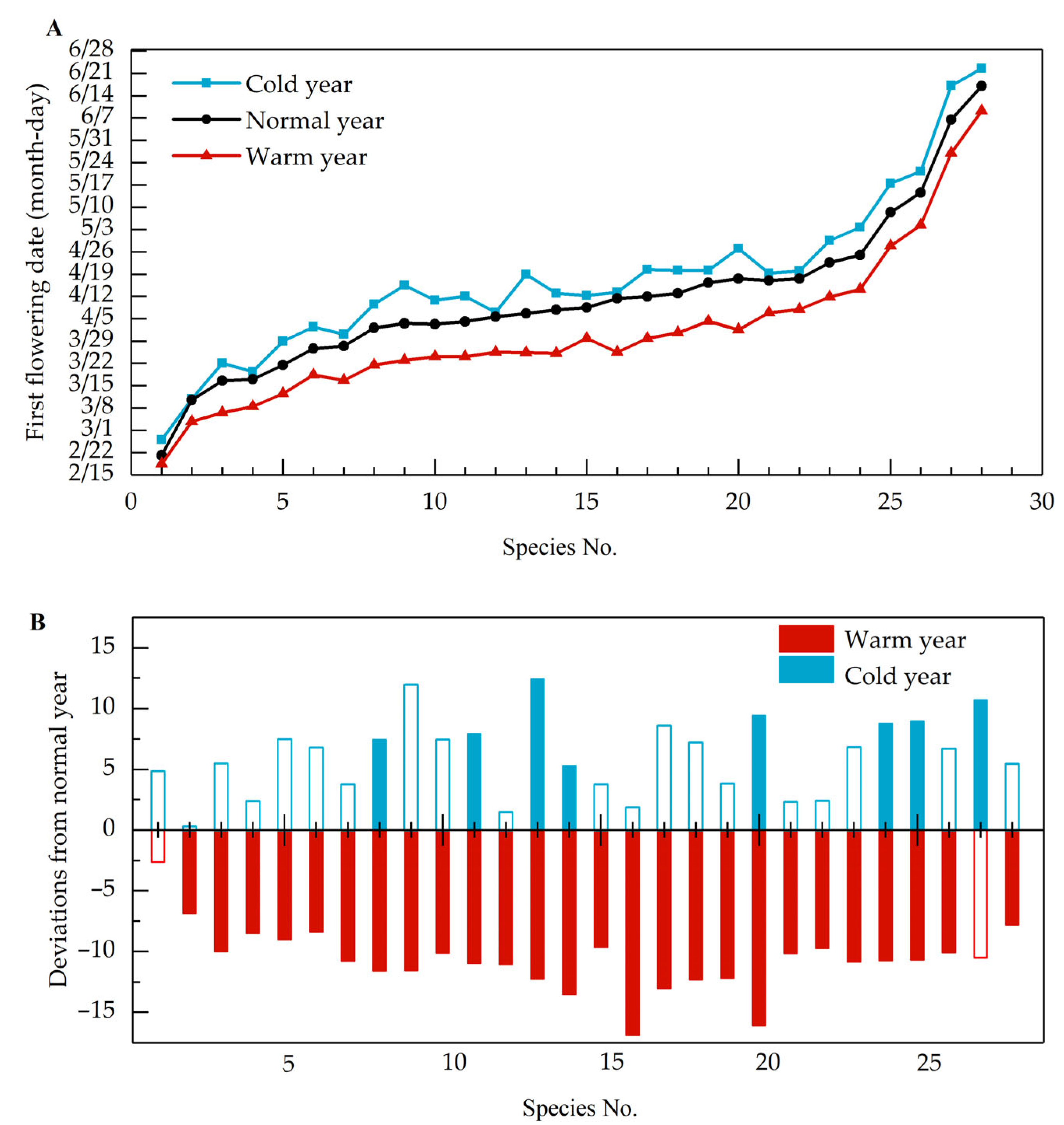
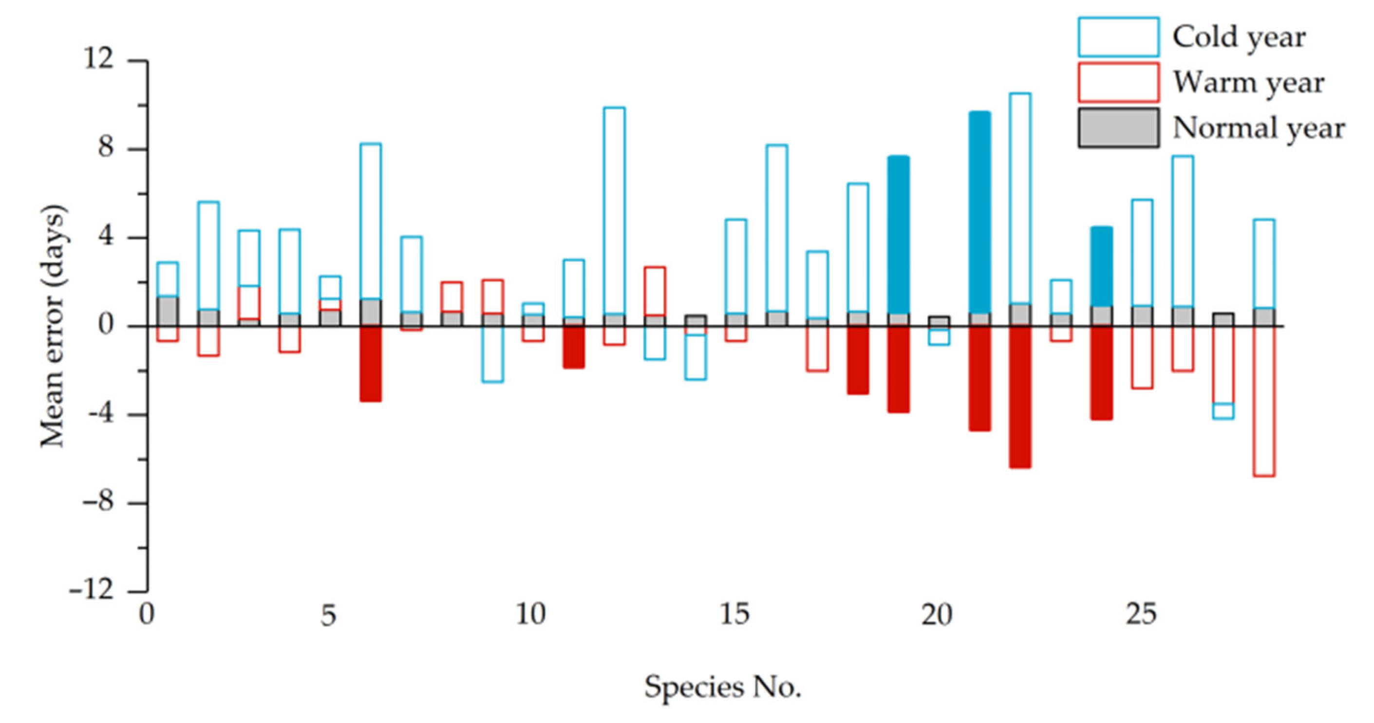
3.1. Phenological Shifts in Years with Abnormal Climate

For the 28 ornamental plant species investigated in this study, the mean FFD in warm years was earlier than in normal years (Figure 2A), with an average advancement of 10.63 days. The advancement varied significantly among species, ranging from 2.63 days (Corylus heterophylla) to 16.86 days (Sapium sebiferum) (Figure 2B). A total of 26 species (accounting for 92.86% of all species) exhibited statistically significant differences (p < 0.05) in their mean initial flowering dates between warm years and normal years.
In cold years, all species flowered later than in normal years, with an average delay of 6.14 days (Figure 2A). The smallest delay was observed in Prunus davidiana (0.32 days), while the largest delay occurred in Citrus trifoliata (12.42 days). Only eight species (accounting for 28.57% of all species) showed significant differences (p < 0.05) in the FFD during cold years compared to normal years (Figure 2B).

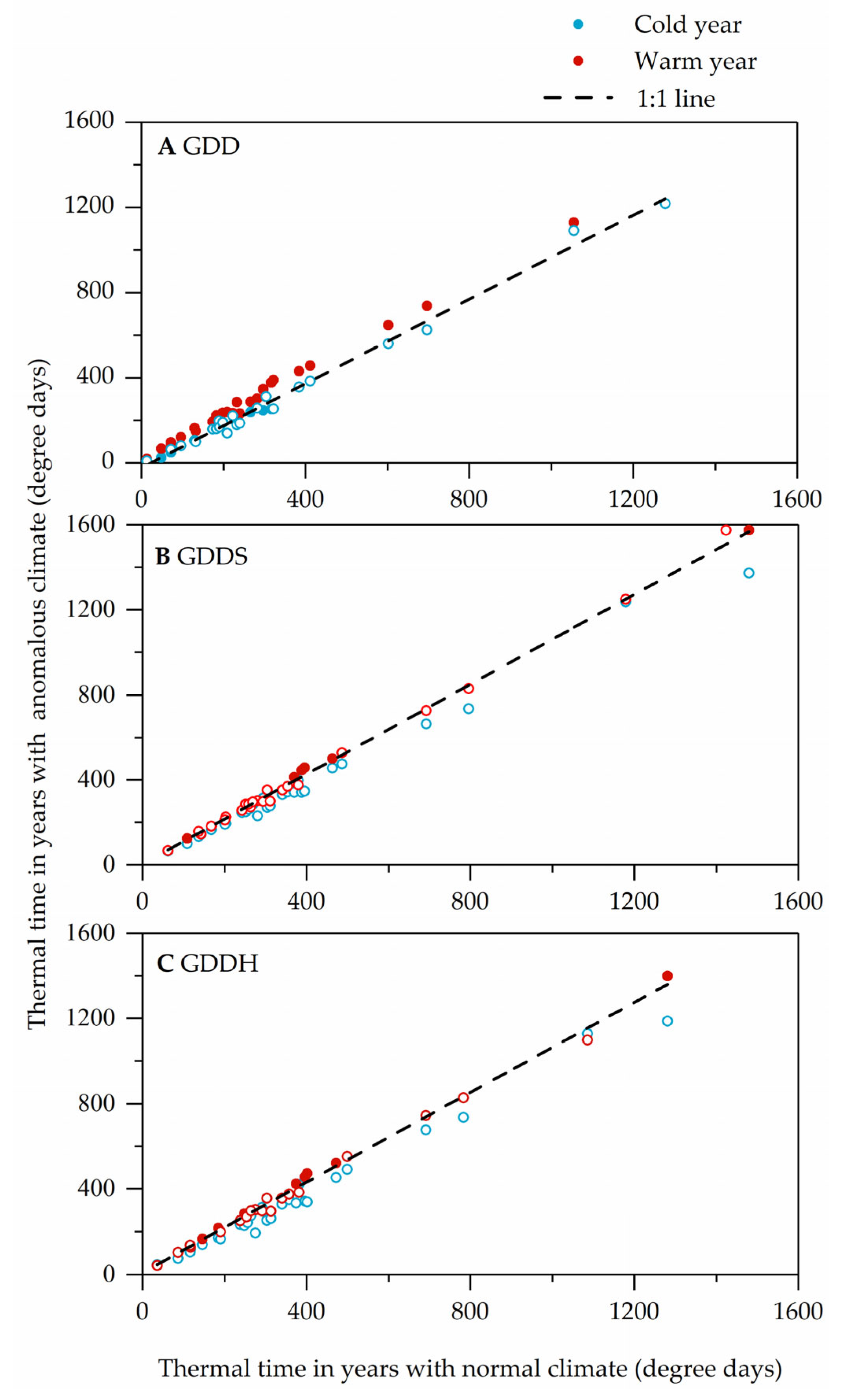
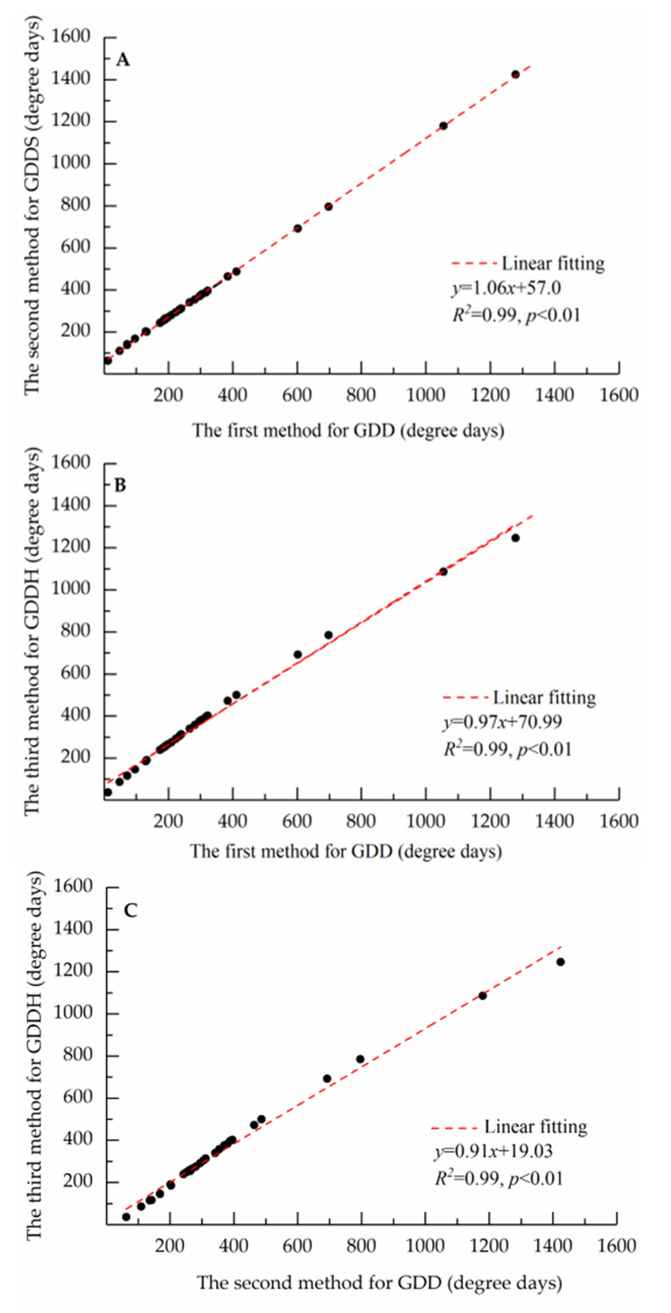
3.2. Changes in Thermal Requirements with Abnormal Climate

Figure 3 illustrates the differences in the thermal requirements of the FFD between abnormal (warm or cold) and normal years. Regardless of the method adopted, all species required higher accumulated temperatures to initiate flowering in warm years compared to normal years. For example, based on method 1, the mean thermal requirement for all species in warm years was 343.05 °C days, significantly higher than the normal-year mean of 308.09 °C days. Similar patterns were observed for methods 2 and 3. Notably, the t-tests revealed that some species exhibited significant differences (p < 0.05) in thermal requirements between warm and normal years (solid circles in Figure 3). Specifically, 39.29% of species showed a significant difference in the FFD based on method 1, while the proportions were slightly lower for method 2 (17.86%) and method 3 (32.14%).
All three methods indicated that the accumulated temperature requirements during cold years were lower than in normal years (Figure 3). For instance, based on method 1, the mean thermal requirement in cold years was 279.19 °C days, lower than 308.09 °C days in normal years. The reduction in the thermal requirement in cold years (28.91 °C days) was slightly smaller than the increase in warm years (34.95 °C days). Although most species required lower accumulated temperatures in cold years, the t-tests identified only five species (Amygdalus davidiana, Yulania denudate, Xanthoceras sorbifolium, Morus alba, and Paeonia suffruticosa) with significant differences based on method 1 (Figure 3A).
A comparison of the three methods (Figure 4) demonstrated that the thermal requirements calculated using them were significantly correlated with each other (R2 > 0.99), but differed in magnitude.

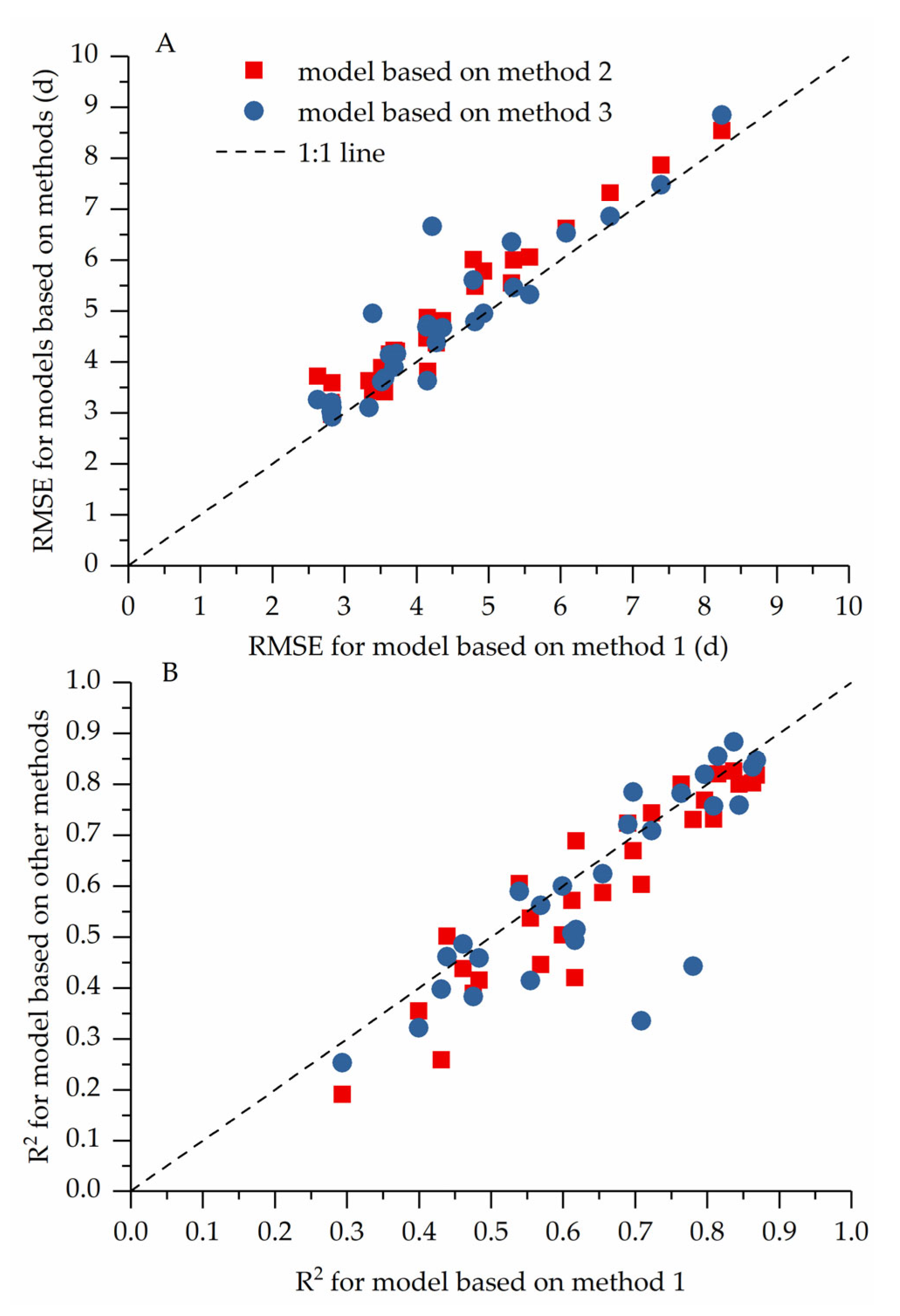
3.3. Model Performance

Using data from normal years, this study calibrated three thermal time models for the FFD of each species (Figure 5). The results demonstrated that these models could generally simulate interannual variance in flowering dates accurately. However, the GDD model based on method 1 had a higher R2 and lower RMSE than the models based on methods 2 and 3 for most species (Figure 5). Therefore, method 1 was selected for subsequent analyses. For the GDD model, the mean goodness of fit (R2) reached 0.64, with all species being significant (p < 0.05). The RMSE ranged from 2.63 days (Forsythia suspensa) to 8.24 days (Ligustrum lucidum), with a mean of 4.40 days across all species.
To evaluate the model performance in abnormal years, the mean errors (simulated FFD minus observed FFD) in normal and abnormal years were calculated (Figure 6). In normal years, the mean errors ranged from 0.33 days to 0.69 days across species, with no significant deviations (p < 0.05). However, in warm years, 23 species (82.14%) showed earlier simulated flowering dates compared to the observations, with the mean errors ranging from −6.75 days to 2.17 days (a mean of −1.57 days for all species). Seven species showed significant errors (differed significantly from zero at p < 0.05), indicating that the model calibrated based on data in normal years overestimated the advancement of the flowering date caused by warming.
In cold years, the mean errors between the simulated FFD and observed FFD ranged from −2.50 days to 9.50 days, with a mean of 3.42 days. Among the 28 ornamental plants investigated, 23 species (82.14%) exhibited a later simulated FFD compared to the observed FFD, with only three species being significant (p < 0.05).

4. Discussion

This study found that climate fluctuations caused significant variance in spring phenology, with the FFDs of 28 ornamental plants in Xi’an advancing by an average of 16.77 days in warm years compared to cold years. The accelerated flowering under warming aligns with previous studies. For example, the impact of urban temperature gradients on the flowering phenology of 10 allergenic tree species (e.g., oaks, elms) in Detroit, MI, USA showed that the elevated temperatures in city centers advanced the flowering dates by 2.5 days per °C compared to suburban areas [39]. Long-term observations (1927–2019) of Jacaranda mimosifolia in three observation stations in Gauteng City, South Africa revealed that a temperature increase of 0.1–0.2 °C per decade significantly advanced flowering, with temperature sensitivity of 4.2–5.3 days per °C [40]. Earlier flowering due to warming may enhance competitive fitness by extending reproductive periods and photosynthetic activity [41,42,43], reflecting plants’ capacity to adapt to climate change. However, earlier spring phenology is not always advantageous. For instance, a study combining field records (1937–2012) and herbarium data (1850–2017) for 68 species in central North America found that advanced flowering increased the frost risk, particularly for spring-flowering plants, potentially damaging flower buds and reducing reproductive success [41].
The results of this study indicate that the thermal requirements for the FFD in ornamental plants were higher in warm years than in normal years, but lower in cold years compared to normal years. These findings align with previous studies on spring phenology. For example, in the US, Fraxinus americana (white ash) exhibited higher accumulated temperature requirements for initial flowering during the anomalously warm year of 2012 compared to other years [24]. The increase in thermal requirements under warm conditions found in this study may be attributed to two factors. The first reason is the reduced winter chilling in warm years. In this study, the autumn–winter temperatures (November–February of the preceding year) in warm years were 1.3 °C higher than in normal years. Thus, accumulated chilling was reduced, and the dormancy release of the flower bud may have been incomplete, causing the bud to require a greater accumulated temperature to burst. The negative correlation between the thermal requirements for leaf unfolding or flowering and the amount of chilling during the preceding autumn and winter was also confirmed by previous studies. For instance, the accumulated temperature required for peach (Prunus persica (L.) Batsch) flowering decreased exponentially with an increased number of chilling days during autumn and winter (days with mean temperatures between 0 and 7.2 °C) in Nanjing, China [26]. Similarly, a study on grapevines (Vitis vinifera) in Japan demonstrated that more chilling reduced the accumulated temperature needed for budburst [44]. The second possible factor is the influence of the photoperiod on flowering dates. In cold years, the delayed flowering date was associated with a longer daylength, and a longer daylength might increase the developmental rate, thus reducing the thermal requirements of the FFD. Based on this assumption, several phenological models (called photothermal time models) accumulate the photoperiod-adjusted temperature [45,46]. However, controlled experiments showed that increased chilling promoted budbreak in all 36 woody species investigated in Germany, whereas an altered daylength only affected the budbreak date in approximately one-third of species [47]. This suggests that chilling outweighs the photoperiod in affecting the spring development of buds. Thus, we did not use the photothermal time model in this study.
Thus far, many studies have employed conventional process-based GDD models to predict spring phenology in woody plants [7,48]. However, conventional GDD models are typically validated using all input data together, without considering their predictive performance under abnormal climatic conditions. In this study, the GDD model calibrated with normal-year phenological data estimated a significantly earlier FFD compared to the observed dates. This discrepancy arose because the thermal requirements in warm years were notably higher than in normal years. In the current terrestrial biosphere models, traditional GDD models remain dominant in predicting the start of the growing season [49,50]. Under future climate warming scenarios, such models may generate substantial errors in predicting phenology and even vegetation productivity. Several phenological models have already incorporated the influence of winter chilling on thermal requirements [20,51]. It is recommended that future generations of terrestrial biosphere models adopt phenological models that account for changes in thermal requirements.

5. Conclusions

Based on the first flowering date (FFD) records of 28 ornamental plants in Xi’an, China and associated meteorological data, we found that climatic fluctuations significantly affected the FFDs and associated thermal requirements of ornamental plants in urban areas. The FFDs of all woody plants were earlier by an average of 10.63 days in warm years compared to normal years, while they were delayed by 6.14 days in cold years. In warm years, most species exhibited higher thermal requirements for the FFD than in normal years, while, in colder years, they displayed lower thermal requirements. The most likely reason is that higher winter temperatures in warm years reduced chilling exposure; then, incomplete dormancy release limited the later developmental rates of flower buds in subsequent springs.
The thermal time model would predict a biased FFD under abnormal climatic conditions. Specifically, the FFD simulated by the thermal time model was earlier by an average of 1.56 days compared to the observed dates in warm years, because conventional thermal time models assume static thermal requirements across years. Given the continued global warming and increased frequency of heat events expected in the future, coupled with intensified urbanization and associated heat island effects, future predictions of the flowering dates of ornamental plants in urban areas must account for warming-induced changes in thermal requirements; otherwise, the impacts of climate warming on flowering dates will be overestimated.

Author Contributions

Conceptualization, methodology, formal analysis, writing—original draft, W.H.; validation, data curation, X.G. and Z.T.; supervision, Z.T. and J.D. All authors have read and agreed to the published version of the manuscript.

Funding

This research was supported by the Academic Research Projects of Beijing Union University (No. ZK20202208); the National Natural Science Foundation of China (Grant No. 42271062); and the Natural Science Foundation of Shandong Province, China (ZR2024QD284).

Data Availability Statement

The original contributions presented in the study are included in the article; further inquiries can be directed to the corresponding author.

Conflicts of Interest

The authors declare no conflicts of interest.

References

  1. Intergovernmental Panel on Climate Change. Climate Change 2021—The Physical Science Basis: Working Group I Contribution to the Sixth Assessment Report of the Intergovernmental Panel on Climate Change; Cambridge University Press: Cambridge, UK, 2021. [Google Scholar]
  2. Schillerberg, T.A.; Tian, D. Global Assessment of Compound Climate Extremes and Exposures of Population, Agriculture, and Forest Lands Under Two Climate Scenarios. Earth’s Future 2024, 12, e2024EF004845. [Google Scholar] [CrossRef]
  3. Cheng, S.; Wang, S.; Li, M.; He, Y. Summer heatwaves in China during 1961–2021: The impact of humidity. Atmos. Res. 2024, 304, 107366. [Google Scholar] [CrossRef]
  4. Zhang, Y.; Zhang, J.; Xia, J.; Guo, Y.; Fu, Y.H. Effects of Vegetation Phenology on Ecosystem Water Use Efficiency in a Semiarid Region of Northern China. Front. Plant Sci. 2022, 13, 945582. [Google Scholar]
  5. Zhou, S.; Yu, B.; Zhang, Y. Global concurrent climate extremes exacerbated by anthropogenic climate change. Sci. Adv. 2023, 9, eabo1638. [Google Scholar] [CrossRef]
  6. Zhao, D.; Zhang, Z.; Zhang, Y. Soil Moisture Dominates the Forest Productivity Decline During the 2022 China Compound Drought-Heatwave Event. Geophys. Res. Lett. 2023, 50, e2023GL104539. [Google Scholar] [CrossRef]
  7. Lyu, J.; Shi, Y.; Liu, T.; Xu, X.; Liu, S.; Yang, G.; Peng, D.; Qu, Y.; Zhang, S.; Chen, C.; et al. Extreme drought-heatwave events threaten the biodiversity and stability of aquatic plankton communities in the Yangtze River ecosystems. Commun. Earth Environ. 2025, 6, 171. [Google Scholar] [CrossRef]
  8. Vieira, J.; Matos, P.; Mexia, T.; Silva, P.; Lopes, N.; Freitas, C.; Correia, O.; Santos-Reis, M.; Branquinho, C.; Pinho, P. Green spaces are not all the same for the provision of air purification and climate regulation services: The case of urban parks. Environ. Res. 2018, 160, 306–313. [Google Scholar] [CrossRef]
  9. Martilli, A.; Krayenhoff, E.S.; Nazarian, N. Is the Urban Heat Island intensity relevant for heat mitigation studies? Urban Clim. 2020, 31, 100541. [Google Scholar] [CrossRef]
  10. Raciti, S.M.; Hutyra, L.R.; Newell, J.D. Mapping carbon storage in urban trees with multi-source remote sensing data: Relationships between biomass, land use, and demographics in Boston neighborhoods. Sci. Total Environ. 2014, 500–501, 72–83. [Google Scholar] [CrossRef]
  11. Song, J.; Zhou, S.; Yu, B.; Li, Y.; Liu, Y.; Yao, Y.; Wang, S.; Fu, B. Serious underestimation of reduced carbon uptake due to vegetation compound droughts. NPJ Clim. Atmos. Sci. 2024, 7, 23. [Google Scholar] [CrossRef]
  12. Ghanbari, M.; Arabi, M.; Georgescu, M.; Broadbent, A.M. The role of climate change and urban development on compound dry-hot extremes across US cities. Nat. Commun. 2023, 14, 3509. [Google Scholar] [CrossRef] [PubMed]
  13. Ge, Q.; Wang, H.; Rutishauser, T.; Dai, J. Phenological response to climate change in China: A meta-analysis. Glob. Chang. Biol. 2015, 21, 265–274. [Google Scholar] [CrossRef] [PubMed]
  14. Huang, Z.; Zhou, L.; Zhong, D.; Liu, P.; Chi, Y. Declined benefit of earlier spring greening on summer growth in northern ecosystems under future scenarios. Agric. For. Meteorol. 2024, 351, 110019. [Google Scholar] [CrossRef]
  15. Meng, L.; Mao, J.; Zhou, Y.; Richardson, A.D.; Lee, X.; Thornton, P.E.; Ricciuto, D.M.; Li, X.; Dai, Y.; Shi, X.; et al. Urban warming advances spring phenology but reduces the response of phenology to temperature in the conterminous United States. Proc. Natl. Acad. Sci. USA 2020, 117, 4228–4233. [Google Scholar] [CrossRef]
  16. Han, G.; Xu, J. Land Surface Phenology and Land Surface Temperature Changes Along an Urban–Rural Gradient in Yangtze River Delta, China. Environ. Manag. 2013, 52, 234–249. [Google Scholar] [CrossRef] [PubMed]
  17. Huang, W.; Dai, J.; Wang, W.; Li, J.; Feng, C.; Du, J. Phenological changes in herbaceous plants in China’s grasslands and their responses to climate change: A meta-analysis. Int. J. Biometeorol. 2020, 64, 1865–1876. [Google Scholar] [CrossRef]
  18. Wang, H.; Zhong, S.; Tao, Z.; Dai, J.; Ge, Q. Changes in flowering phenology of woody plants from 1963 to 2014 in North China. Int. J. Biometeorol. 2019, 63, 579–590. [Google Scholar] [CrossRef]
  19. Guralnick, R.; Crimmins, T.; Grady, E.; Campbell, L. Phenological response to climatic change depends on spring warming velocity. Commun. Earth Environ. 2024, 5, 634. [Google Scholar] [CrossRef]
  20. Lin, S.; Wang, H.; Ge, Q.; Hu, Z. Effects of chilling on heat requirement of spring phenology vary between years. Agric. For. Meteorol. 2022, 312, 108718. [Google Scholar] [CrossRef]
  21. Rauschkolb, R.; Herben, T.; Kattge, J.; Knickmann, B.; Linstädter, A.; Menzel, A.; Mora, K.; Nordt, B.; Vitasse, Y.; Weigelt, P.; et al. The performance of growing degree day models to predict spring phenology of herbaceous species depends on the species’ temporal niche. Funct. Ecol. 2025. [Google Scholar] [CrossRef]
  22. Wheeler, K.I.; Dietze, M.C.; LeBauer, D.; Peters, J.A.; Richardson, A.D.; Ross, A.A.; Thomas, R.Q.; Zhu, K.; Bhat, U.; Munch, S.; et al. Predicting spring phenology in deciduous broadleaf forests: NEON phenology forecasting community challenge. Agric. For. Meteorol. 2024, 345, 109810. [Google Scholar] [CrossRef]
  23. Clark, J.S.; Salk, C.; Melillo, J.; Mohan, J. Tree phenology responses to winter chilling, spring warming, at north and south range limits. Funct. Ecol. 2014, 28, 1344–1355. [Google Scholar] [CrossRef]
  24. Carter, J.M.; Orive, M.E.; Gerhart, L.M.; Stern, J.H.; Marchin, R.M.; Nagel, J.; Ward, J.K. Warmest extreme year in U.S. history alters thermal requirements for tree phenology. Oecologia 2017, 183, 1197–1210. [Google Scholar] [CrossRef]
  25. Hsu, H.; Yun, K.; Kim, S. Variable warming effects on flowering phenology of cherry trees across a latitudinal gradient in Japan. Agric. For. Meteorol. 2023, 339, 109571. [Google Scholar] [CrossRef]
  26. Yan, J.; Cai, Z.; Chen, Z.; Zhang, B.; Li, J.; Xu, J.; Ma, R.; Yu, M.; Shen, Z. Relationship between Chilling Accumulation and Heat Requirement for Flowering in Peach Varieties of Different Chilling Requirements. Agronomy 2024, 14, 1637. [Google Scholar] [CrossRef]
  27. Zhang, P.; Ning, P.; Cao, R.; Xu, J. Analysis of Climate Change Characteristics in Xi’an Based on the Visibility Graph. Front. Phys. 2021, 9, 702064. [Google Scholar] [CrossRef]
  28. Wang, C.; Zhang, H.; Ma, Z.; Yang, H.; Jia, W. Urban Morphology Influencing the Urban Heat Island in the High-Density City of Xi’an Based on the Local Climate Zone. Sustainability 2024, 16, 3946. [Google Scholar] [CrossRef]
  29. Wan, M.; Liu, X. Zhong Guo Wu Hou Guan Ce Fang Fa; Science Press: Beijing, China, 1979. [Google Scholar]
  30. Chow, D.; Levermore, G.J. New algorithm for generating hourly temperature values using daily maximum, minimum and average values from climate models. Build. Serv. Eng. Res. Technol. 2007, 28, 237–248. [Google Scholar] [CrossRef]
  31. Shahzad, K.; Zhu, M.; Cao, L.; Hao, Y.; Zhou, Y.; Liu, W.; Dai, J. Phylogenetic conservation in plant phenological traits varies between temperate and subtropical climates in China. Front. Plant Sci. 2024, 15, 1367152. [Google Scholar] [CrossRef]
  32. Hunter, A.F.; Lechowicz, M.J. Predicting the Timing of Budburst in Temperate Trees. J. Appl. Ecol. 1992, 29, 597–604. [Google Scholar] [CrossRef]
  33. Cannell, M.G.R.; Smith, R.I. Thermal Time, Chill Days and Prediction of Budburst in Picea sitchensis. J. Appl. Ecol. 1983, 20, 951–963. [Google Scholar] [CrossRef]
  34. Sarvas, R. Investigations on the annual cycle of development of forest trees. Active period. Finl. Metsantutkimuslaitos Julk. 1972, 76, 110. [Google Scholar]
  35. Hänninen, H. Modelling bud dormancy release in trees from cool and temperate regions. Acta For. Fenn 1990, 213, 7660. [Google Scholar] [CrossRef]
  36. Anderson, J.; Richardson, E.; Kesner, C. Validation of chill unit and flower bud phenology models for ‘Montmorency’ sour cherry. Acta Hortic. 1986, 184, 71–78. [Google Scholar] [CrossRef]
  37. Luedeling, E.; Zhang, M.; McGranahan, G.; Leslie, C. Validation of winter chill models using historic records of walnut phenology. Agric. For. Meteorol. 2009, 149, 1854–1864. [Google Scholar] [CrossRef]
  38. Menzel, A.; Helm, R.; Zang, C. Patterns of late spring frost leaf damage and recovery in a European beech (Fagus sylvatica L.) stand in south-eastern Germany based on repeated digital photographs. Front. Plant Sci. 2015, 6, 1–13. [Google Scholar] [CrossRef]
  39. Li, D.; Stucky, B.J.; Deck, J.; Baiser, B.; Guralnick, R.P. The effect of urbanization on plant phenology depends on regional temperature. Nat. Ecol. Evol. 2019, 3, 1661–1667. [Google Scholar] [CrossRef]
  40. Fitchett, J.M.; Raik, K. Phenological advance of blossoming over the past century in one of the world’s largest urban forests, Gauteng City-Region, South Africa. Urban For. Urban Green. 2021, 63, 127238. [Google Scholar] [CrossRef]
  41. Austin, M.W.; Smith, A.B.; Olsen, K.M.; Hoch, P.C.; Krakos, K.N.; Schmocker, S.P.; Miller-Struttmann, N.E. Climate change increases flowering duration, driving phenological reassembly and elevated co-flowering richness. New Phytol. 2024, 243, 2486–2500. [Google Scholar] [CrossRef]
  42. Chen, Y.; Yang, X.; Zhang, T.; Zhao, Y.; Sun, Y.; Ma, M. Warming promotes divergent shift in sequential phenophases of alpine meadow plants. Agric. For. Meteorol. 2025, 368, 110521. [Google Scholar] [CrossRef]
  43. Cleland, E.E.; Allen, J.M.; Crimmins, T.M.; Dunne, J.A.; Pau, S.; Travers, S.E.; Zavaleta, E.S.; Wolkovich, E.M. Phenological tracking enables positive species responses to climate change. Ecology 2012, 93, 1765–1771. [Google Scholar] [CrossRef] [PubMed]
  44. Kamimori, M.; Hosomi, A. Evaluation of Chilling and Heat Requirements for the Budbreak of Delaware Grape in Osaka, Japan. Am. J. Enol. Vitic. 2024, 75, 750011. [Google Scholar] [CrossRef]
  45. Mo, Y.; Zhang, J.; Jiang, H.; Fu, Y.H. A comparative study of 17 phenological models to predict the start of the growing season. Front. For. Glob. Chang. 2023, 5, 1032066. [Google Scholar] [CrossRef]
  46. Wang, H.; Lin, S.; Dai, J.; Ge, Q. Modeling the effect of adaptation to future climate change on spring phenological trend of European beech (Fagus sylvatica L.). Sci. Total Environ. 2022, 846, 157540. [Google Scholar] [CrossRef]
  47. Laube, J.; Sparks, T.H.; Estrella, N.; Höfler, J.; Ankerst, D.P.; Menzel, A. Chilling outweighs photoperiod in preventing precocious spring development. Glob. Change Biol. 2014, 20, 170–182. [Google Scholar] [CrossRef]
  48. Zhu, M.; Dai, J.; Wang, H.; Alatalo, J.M.; Liu, W.; Hao, Y.; Ge, Q. Mapping 24 woody plant species phenology and ground forest phenology over China from 1951 to 2020. Earth Syst. Sci. Data 2024, 16, 277–293. [Google Scholar] [CrossRef]
  49. Richardson, A.D.; Anderson, R.S.; Arain, M.A.; Barr, A.G.; Bohrer, G.; Chen, G.; Chen, J.M.; Ciais, P.; Davis, K.J.; Desai, A.R.; et al. Terrestrial biosphere models need better representation of vegetation phenology: Results from the North American Carbon Program Site Synthesis. Glob. Chang. Biol. 2012, 18, 566–584. [Google Scholar] [CrossRef]
  50. Zhang, R.; Wang, F.; Zheng, J.; Chen, L.; Hänninen, H.; Wu, J. Temperature sum models in plant spring phenology studies: Two commonly used methods have different fields of application. J. Exp. Bot. 2024, 75, 6011–6016. [Google Scholar] [CrossRef]
  51. Zhang, H.; Liu, S.; Regnie, P.; Yuan, W. New insights on plant phenological response to temperature revealed from long-term widespread observations in China. Glob. Chang. Biol. 2018, 24, 2066–2078. [Google Scholar] [CrossRef]
Figure 1. Classification of cold, warm, and normal years. (A) The March to May average temperature from 1963 to 2018; (B) the comparison of the daily mean temperature averaged from years with abnormal and normal climates. The gray-shaded areas denote March to May.
Horticulturae 11 00772 g001
Figure 2. The difference in the first flowering date (FFD) between the years with an abnormal and normal climate in Xi’an. (A) The average FFD in cold years, normal years, and warm years for each species; (B) the difference in the FFD between years with abnormal and normal climates. The solid bars indicate that the difference is significant (p < 0.05).
Horticulturae 11 00772 g002
Figure 3. The comparison of the thermal requirements for the first flowering date (FFD) between years with an abnormal and normal climate in Xi’an. (A) The results of the first method; (B) the results of the second method; (C) the results of the third method. The solid circles indicate that the difference is significant (p < 0.05).
Horticulturae 11 00772 g003
Figure 4. The comparisons among different methods for the calculation of thermal requirements. (A) Method 1 vs. method 2; (B) method 1 vs. method 3; (C) method 2 vs. method 3. Black circles represent the mean thermal requirement in normal years for each species.
Horticulturae 11 00772 g004
Figure 5. Comparisons of the effects of the thermal time model in simulating the first flowering dates of 28 ornamental species in Xi’an. (A) RMSE of model based on method 1 vs. methods 2 and 3; (B) R2 of model based on method 1 vs. methods 2 and 3.
Horticulturae 11 00772 g005
Figure 6. The error of the model in simulating the FFD in years with an abnormal and normal climate. The solid bars indicate that the mean error was significantly different from 0 (p < 0.05).
Horticulturae 11 00772 g006
Table 1. Summary of ornamental species investigated in this study.
No.SpeciesLife FormProvenanceNFirst Flowering Date (Month-Day)
1Corylus heterophyllaShrub or small treeTemperate322-21
2Amygdalus davidianaTreeTemperate433-9
3Forsythia suspensaShrubTemperate323-14
4Yulania denudateTreeSubtropical423-16
5Cerasus tomentosaShrubTemperate323-20
6Pyrus betulifoliaTreeTemperate323-25
7Cerasus yedoensisTreeTemperate413-26
8Syringa oblataShrub or small treeTemperate444-1
9Pterocarya stenopteraTreeSubtropical324-2
10Acer pictum subsp. monoTreeTemperate424-2
11Cercis chinensisShrubTemperate434-3
12Chaenomeles sinensisShrub or small treeSubtropical344-3
13Poncirus trifoliataSmall treeSubtropical344-5
14Fraxinus chinensisTreeTemperate304-6
15Juglans regiaTreeTemperate384-7
16Platanus orientalisTreeTemperate304-9
17Xanthoceras sorbifoliumShrub or small treeTemperate324-9
18Wisteria sinensisLianaSubtropical374-11
19Morus albaTreeTemperate344-14
20Broussonetia papyriferaTreeSubtropical304-15
21Paeonia suffruticosaShrubTemperate424-15
22Pinus tabuliformisTreeTemperate364-16
23Cornus controversaTreeSubtropical324-21
24Robinia pseudoacaciaTreeTemperate414-24
25Diospyros kakiTreeSubtropical385-8
26Ailanthus altissimaTreeTemperate365-14
27Albizia julibrissinTreeTemperate346-7
28Ligustrum lucidumTreeSubtropical326-16
The first flowering date is the multi-year average. N, number of observation years.
Disclaimer/Publisher’s Note: The statements, opinions and data contained in all publications are solely those of the individual author(s) and contributor(s) and not of MDPI and/or the editor(s). MDPI and/or the editor(s) disclaim responsibility for any injury to people or property resulting from any ideas, methods, instructions or products referred to in the content.

