Article

A Two-Stage Canopy Extraction Method Utilizing Multispectral Images to Enhance the Estimation of Canopy Nitrogen Content in Pear Orchards with Full Grass Cover

1
Institute of Agricultural Facilities and Equipment, Jiangsu Academy of Agricultural Sciences, Nanjing 210014, China
2
Key Laboratory of Horticultural Equipment, Ministry of Agriculture and Rural Affairs, Nanjing 210014, China
*
Author to whom correspondence should be addressed.
Horticulturae 2025, 11(12), 1419; https://doi.org/10.3390/horticulturae11121419
Submission received: 30 September 2025 / Revised: 27 October 2025 / Accepted: 13 November 2025 / Published: 24 November 2025
(This article belongs to the Special Issue New Trends in Smart Horticulture)

Abstract

Accurately extracting the canopies of fruit trees is crucial to improve the estimation accuracy of CNC inversion as well as determine a reasonable application of nitrogen fertilizer. To date, existing studies have mainly focused on canopy extraction in scenarios with no grass or sparse grass cover, paying less attention to scenarios with a full grass cover. Thus, in this paper, a two-stage canopy extraction (TCE) method was proposed to address the issue of canopy extraction in scenarios with full grass cover. Firstly, the height difference between the canopies of pear trees and the ground grass was used to eliminate the interference of the ground grass and achieve a coarse-grained canopy extraction. Then, based on the extracted coarse-grained canopies and CIELAB color space, the color thresholds of the L*, a*, and b* channels were determined to remove the interference factors, e.g., branches, shadows, and trellises, for fine-grained canopy extraction by using data distribution from the three channels based on a histogram and the threshold of confidence interval. In canopy extraction experiments, the accuracy, recall, precision, and F1-score of TCE in scenarios with full grass cover can reach 91.725%, 95.789%, 91.284%, and 93.482%, respectively, demonstrating the effectiveness of TCE in addressing canopy extraction issues in this scenario. Thirdly, the RF algorithm was utilized to select suitable VIs based on R2 and RMSE values, and CNC inversion models were constructed. In estimation experiments on CNC inversion, the R2, RMSE, and nRMSE of the constructed CNC inversion based on TCE in a scenario with full grass cover were 0.724, 0.243, and 19.120%, respectively. A comparative analysis with the baseline method revealed that accurate canopy extraction contributed to a high estimation accuracy of CNC inversion. Therefore, our proposed method can provide technical support for the efficient and non-destructive monitoring of the canopy nutrient status in pear orchards.

1. Introduction

Nitrogen is an essential nutrient for the growth and development of pear trees. The precise management of nitrogen fertilizer can significantly enhance the quality of pears and prevent the waste and pollution resulting from excessive application [1]. To achieve precise management, it is necessary to assess the nutritional status of pear trees. Canopy nitrogen content (CNC), as a critical indicator, can reflect the overall nitrogen status of pear trees [2].
Currently, compared to traditional measurement methods, e.g., the Kjeldahl method [3], the spectral imaging method using unmanned aerial vehicles (UAVs) has shown promise as a prospective technology for this application due to its superiority in rapid, non-destructive, and dynamic monitoring [4]. Existing studies on CNC have mainly aimed to measure field crops, e.g., rice [5], wheat [6], and maize [7], as well as some horticultural crops, e.g., apple [8], litchi [9], and banana [10]. Constructing new vegetation indexes (VIs), e.g., abundance adjusted VIs (AAVIs) [5], and utilizing multi-feature fusion, e.g., spectral information [6] and canopy texture [10], are the most commonly used methods to improve the estimation of CNC inversion. However, due to the improvement of agronomic management, challenges still exist in accurately extracting individual tree information from spectral images, which hinders the rapid and precise estimation of CNC for pear trees.
In previous studies, the canopy extraction of fruit trees from UAV spectral images has often depended on the index threshold (IT) method, which is based on spectral reflectance [8,9,10,11,12,13,14], and the target classification (TC) method, which is based on RGB images [15,16,17,18], as illustrated in Table 1. These studies have successfully achieved precise canopy extractions of fruit trees in scenarios with no grass or sparse grass cover. However, they have paid less attention to those with full grass cover, e.g., pear orchards with grass coverage management. In modern pear orchards, grass coverage management has increasingly become a sustainable practice to enhance soil fertility, reduce water and soil erosion, and improve biodiversity and ecosystem services [19,20]. Although it offers numerous agronomic benefits, this technology also results in spectral images collected from UAVs containing more complex and similar background information. Thus, this new scenario with full grass cover poses new challenges for existing methods aiming at precisely extracting the canopies of fruit trees.
For IT-based methods, similar index values, e.g., VI and color index (CI), between the grass coverage area and the canopy area pose a challenge for setting the screening threshold [21]. TC-based methods can achieve high-precision extraction, but they rely on complex feature engineering and large-size labeled data [22]. Expanding and marking the dataset in a scenario with full grass cover is a primary task, which would be quite labor-intensive. Meanwhile, due to the limitations of spatial resolution, precisely labeling the grass coverage area and the canopy area is challenging, particularly in areas with blurred boundaries [23]. Furthermore, most existing studies have aimed to segment continuous canopy regions for determining the range of spraying application [14,15,18]. However, canopy extraction for CNC inversion needs to further eliminate interfering factors, e.g., shadows and branches, for enhancing inversion accuracy [16]. The extracted canopy regions could be discontinuous. Therefore, the precise extraction of pear tree canopies to enhance the accuracy of CNC inversion in scenarios with full grass cover needs to be urgently addressed.
At present, in addition to spectral images, UAVs can also synchronously obtain the elevation information of each pixel in the collected images, e.g., through using a digital surface model (DSM) [24]. The height difference between canopy regions and grass-covered regions can offer a novel perspective for initially eliminating background information, thereby achieving the coarse-grained extraction of canopies. However, due to the presence of shadows and branches, the extracted coarse-grained images still require further processing. The color difference is an obvious feature that can be used to eliminate shadows and branches from the extracted coarse-grained canopies, thus achieving the precise canopy extraction of pear trees. To the best of our knowledge, this extraction method has received less attention in the existing literature.
Considering the estimation of CNC, machine learning (ML) algorithms, e.g., random forest (RF), artificial neural network (ANN) [25,26], and support vector machine (SVM), are one of the most commonly used tools for constructing CNC inversion models [27]. They can provide better accuracy for CNC estimation compared with traditional statistical models [28]. Some previous studies have shown that the RF algorithm can better represent the correlation between VIs and CNC [4,29], thereby being helpful for constructing high-precision inversion models. Due to the differences in leaf structure and canopy structure among various fruit trees [30], the sensitive VIs screened out would be different [31]. Thus, to enhance the accuracy of the constructed inversion models, it is necessary to further explore the method of using ML algorithms to invert the CNC in pear orchards.
As a result, to address the issue of canopy extraction in the scenario with full grass cover, this paper proposed a two-stage canopy extraction method (TCE) to achieve high-precision CNC inversion in pear orchards. The specific objectives were to (i) use the height difference between the canopies of pear trees and ground grass to eliminate the interference of ground grass and achieve the coarse-grained canopy extraction; (ii) then, based on the extracted coarse-grained canopies and the CIELAB color space, determine the color thresholds of three channels using the data distribution of L*, a*, and b* based on the histogram and the thresholds of the confidence interval to complete the fine-grained canopy extraction; (iii) screen sensitive VIs and construct CNC inversion models based on the RF; and (iv) quantitatively compare the performance of our proposed canopy extraction method and the constructed CNC inversion models with baseline methods.
This paper is organized into four sections. Section 2 introduces the study areas, data collection and preprocessing, canopy extraction method, and construction of the inversion model. Section 3 mainly shows the experimental results to compare the performance of our proposed method under different grass cover densities. Section 4 discusses the findings in depth through analyzing the experimental results and highlights the future research directions. The conclusions are presented in Section 5.

2. Materials and Methods

2.1. Study Areas

This study was conducted across two pear orchards situated in Jiangsu Province, China (Figure 1a): the Jiangsu Academy of Agricultural Sciences (JAAS) pear orchard (Figure 1b, 118°52′16″ E, 32°2′16″ N) and the Yejia pear orchard (Figure 1c, 120°6′2″ E, 32°18′55″ N). These two regions boast a subtropical monsoon climate with an annual average sunshine duration ranging from 2125 to 2182.4 h and an average temperature ranging from 14.9 to 15.4 °C. These favorable climatic and geographic conditions have a significant impact on the flourishing fruit tree cultivation industry. The two pear orchards were constructed in accordance with the requirement of modern standardized orchards. Pear trees were planted at equal intervals and managed by professionals. The experimental regions of the JAAS orchard and the Yejia pear orchard are shown in Figure 1b,c, and their areas are 16.15 ha and 18.39 ha, respectively. The red outlines in Figure 1b,c were used to visualize the experimental results, e.g., canopy extraction and CNC distribution.

2.2. Data Collection and Preprocessing

2.2.1. Canopy-Scale Data Collection and Preprocessing

A DJI Mavic 3 (multispectral version UAV, SZ DJI Technology Co., Shenzhen, Guangdong, China) was used to acquire multispectral images, including 4 bands: green band (544–576 nm), red band (634–666 nm), red edge (714–746 nm), and near-infrared (834–886 nm), as well as one panchromatic band. The visible light camera and multispectral camera are 4/3 CMOS with 20 million pixels and 1/2.8-inch CMOS with 5 million pixels, respectively. The maximum horizontal flight speed and takeoff altitude are 15 m/s and 6000 m. To eliminate radiation interference, the spectral image of a standard white board was first collected for radiometric correction. The flight missions of the UAV can cover the experimental orchards and automatically plan trajectories. The flight parameters settings were 30 m above the ground, a cruising speed of 2 m/s, a side overlap rate of 70%, a course overlap rate of 80%, and a ground spatial resolution of 0.8 cm/pixel. In this paper, to verify the canopy extraction performance of pear trees under different grass cove densities, three groups of multispectral images were collected in the JAAS pear orchard on 18 June 2024, 5 July 2024, and 12 June 2025, corresponding to the scenarios with no grass, sparse grass coverage, and full grass cover, respectively, as shown in Figure 2. A group of multispectral images were collected in the Yejia pear orchard with full grass cover on 17 June 2025. During these collection processes, the weathers was all clear with low wind speed. The specific collection times were all between 10 am and 2 pm. The collected multispectral images were preprocessed with the DJI Terra software (version 4.5, SZ DJI Technology Co., Shenzhen, Guangdong, China) via radiometric correction and image stitching.

2.2.2. Leaf-Scale Data Collection and Preprocessing

While the UAV was collecting multispectral images, leaf-scale data, including leaf nitrogen content (LNC) and leaf area index (LAI), were simultaneously collected. Specifically, a total of 340 pear trees were randomly selected to collect leaf-scale data at the four time points of multispectral image acquisition. The selected pear trees were manually numbered to match their positions in the multispectral images. For each pear tree, a total of 10 healthy and undamaged pear leaves were randomly selected from its canopy to measure their LNC using a TYS-4N plant nutrition tester (Zhejiang Top Cloud-agri Technology Co., Ltd, Hangzhou, Zhejiang, China). The maximum value and accuracy of the TYS-4N for nitrogen measurement are 99.9 mg/g and ± 0.5 mg/g. The LNC of each leaf was measured three times along the direction from the top to the petiole of the leaf. The average of the three measurements represented the LNC of a single leaf. The average of the LNC of ten leaves was the LNC of each pear tree. The LAI was measured using the LAI-2200 Plant Canopy Analyzer (PCA) (LI-COR Inc., Lincoln, NE, USA) from four different directions below the canopy of each pear tree. The collection at each measurement point was conducted three times, and the average value was taken as the LAI of the measured pear tree. The CNC of each pear tree (the measured CNC) can be calculated by Equation (1) [32]. The mathematical statistics for the LNC, LAI, and CNC are listed in Table 2.
C N C = L N C × L A I

2.3. Principle of Two-Stage Canopy Extraction Method

2.3.1. Coarse-Grained Canopy Extraction Based on Height Difference

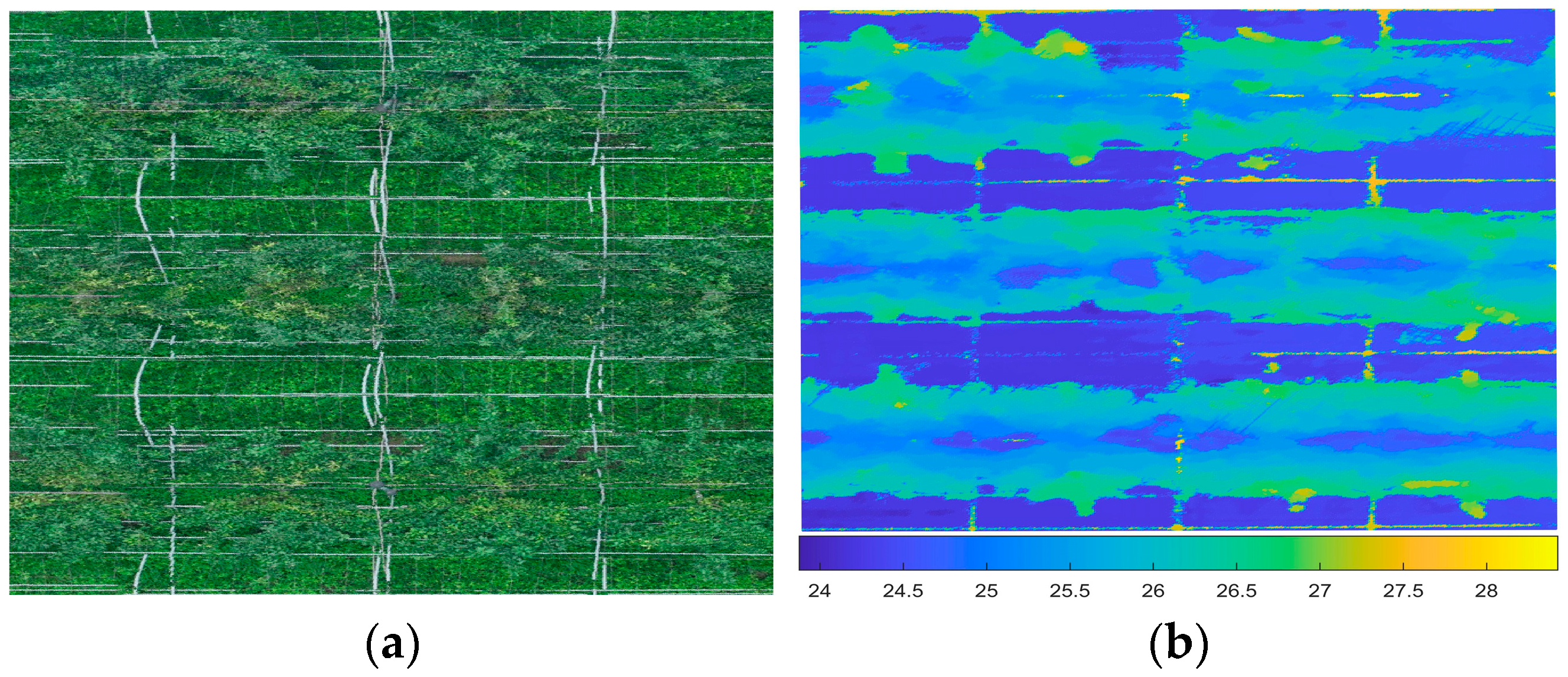
As shown in Figure 3a, it is hardly to directly classify the canopy area and the grass-covered area visually. But, their height difference (Figure 3b) is an obvious characteristic for distinguishing these two areas in the scenario with full grass cover. Thus, the DSM image, which contains the elevation information of each pixel, is an important tool for eliminating complex ground background information. The process for canopy extraction based on height difference was as follows: (i) The height thresholds, representing the distance from the first fork point of each pear tree’s main trunk to the ground, were measured with a steel tape measure; (ii) In the DSM image, the valid pixels in the subarea of each pear tree were selected based on the measured height thresholds using the traversal approach [33]. The subarea of each pear tree refers to the division formed by the trellis structure of the pear orchard. Thus, the canopies of pear trees were separated from the complex background information through binary classification. It is worth noting that the extracted canopies of the pear trees were coarse-grained. They still contained some interference factors, i.e., shadows, branches, and trellises. The selection rule was expressed as Equation (2). Furthermore, all data processing in this paper was carried out in MATLAB (version R2023b, The MathWorks Inc., Natick, MA, USA).
P i x e l h   ( x , y ) = 0 , h ( x , y )   h t 1 , h ( x , y ) > h t
where P i x e l h ( x , y ) is the set value of the pixel at coordinate ( x , y ) via height selection. h ( x , y ) is the height value of the pixel at coordinate ( x , y ) in the DSM data. h t is the measured height threshold and uniformly set as 24.5 cm. While h ( x , y ) h t , the pixel at coordinate ( x , y ) is defined as an invalid pixel, and its value is set to 0. Otherwise, the pixel is a valid pixel, and its value is set to 1.

2.3.2. Fine-Grained Canopy Extraction Based on Color Thresholds

Based on the extracted coarse-grained canopy, shadows, branches, and trellises need to be further eliminated. Upon analysis, there is a clear color difference between the leaves and these interference factors. Thus, the color differences were used for fine-grained canopy extraction. The process for fine-grained canopy extraction based on color difference was as follows. (i) Pixel alignment between different images. Due to the accuracy differences of the used sensors, three types of preprocessed images—RGB images, grayscale images, and DSM images—had different resolutions. Thus, the resize () function of MATLAB was adopted to unify the resolution of these images to achieve the alignment of each pixel position. (ii) Conversion of color spaces. To eliminate the interference factors, the CIELAB color space was used to perceive the lightness of each pixel through converting the R, G, and B channels into the L*, a*, and b* channels [34]. In this color space, the L* channel indicates the lightness, which is the main basis for eliminating shadows. The a* channel describes the color change on the red–green axis. Its positive and negative values represent red and green colors, respectively. The positive and negative values of the b* channel are yellow and blue colors, respectively. (iii) Determine the three-channel thresholds. Due to the differences in sunlight brightness and CNC, the screening thresholds for the L*, a*, and b* channels are not fixed values. Thus, they need to be dynamically decided according to the actually collected data. The screening thresholds for each channel were determined by analyzing the histogram of the three-channel values in the subarea of each pear tree. The screening rule adhered to Equation (3). Based on the above three steps, the canopy of the pear tree can be precisely extracted.
P i x e l c   ( x , y ) = 1 ,   L * ( x , y ) L l * ,   L u * ,   a * ( x , y ) a l * ,   a u * ,   b * ( x , y ) b l * ,   b u * 0 , o t h e r w i s e  
where P i x e l c   ( x , y ) is the set value of the pixel at coordinate ( x , y ) via color selection. L * ( x , y ) , a * ( x , y ) , and b * ( x , y ) represent the value of L*, a*, and b* at coordinate ( x , y ) in RGB image, respectively. L l * , a l * , and b l * represent the lower limit threshold for screening L*, a*, and b*. L u * , a u * , and b u * represent the higher limit threshold for screening L*, a*, and b*. While the value of L*, a*, and b* simultaneously satisfy their threshold range, the pixel at coordinate ( x , y ) is defined as a valid pixel, and its value is set to 1. Otherwise, the pixel is an invalid pixel, and its value is set to 0.

2.3.3. Baseline Methods

To test the effectiveness of our proposed method (TCE), in this section, three baseline methods were designed and introduced.
The manual pixel filtering method (MPF) utilized the box selection tool in ArcGIS Pro software (version 10.8, Esri Inc, Redlands, CA, USA) [18] to manually remove the pixels outside the canopy area, e.g., those representing leaf shadows, branches, grass, and trellis. Theoretically, the canopy extracted by this method is the most accurate. Thus, this method is taken as the basis for calculating accuracy indicators.
The texture feature-based segmentation method (TFS) was used to illustrate the canopy extraction effects of the TC method based on RGB images. The gray-level co-occurrence matrix (GLCM) is the most widely used approach for texture feature extraction [35]. In this paper, eight commonly used texture features, including Mean, Variance, Synergy, Contrast, Dissimilarity, Entropy, Second-order Moment and Correlation, were extracted from the R, G, and B channels. Furthermore, the k-mean clustering algorithm was used for target classification [36].
The index threshold-based extraction method (ITE) was applied to show the canopy extraction effects of the IT method based on spectral reflectance. Upon consulting the existing literature, we found that the Modified Soil-Adjusted Vegetation Index (MSAVI) [37] is one of the most effective VIs for differentiating the canopy area from the background. The canopies of pear trees can be extracted via setting the threshold of MSAVI. The calculation of MSAVI was expressed as Equation (4).
M S A V I = 2 × R N I R + 1 ( 2 × R N I R + 1 ) 2 8 × ( R N I R R R e d ) 2
where R N I R denotes the reflectance of the NIR band. R R e d is the reflectance of the red band.

2.3.4. Accuracy Evaluation for Canopy Extraction

To comprehensively evaluate the performance for canopy extraction among three methods, i.e., TCE, TFS, and ITE, the accuracy (Equation (5)), recall (Equation (6)), precision (Equation (7)), and F1-score (Equation (8)) were involved as evaluation metrics.
A c c u r a c y   ( % ) = T P + T N T P + T N + F P + F N × 100  
R e c a l l   % = T P T P + F N × 100
P r e c i s i o n   % = T P T P + F P × 100
F 1 s c o r e   % = 2 × P r e c i s i o n × R e c a l l P r e c i s i o n + R e c a l l
where TP is the number of true positives; TN is the number of true negatives; FP is the number of false positives; and FN is the number of false negatives.

2.4. Construction of CNC Inversion Model

2.4.1. Calculation and Screening of VIs

VIs can effectively reflect the growth and health status and are one of the most commonly used indexes for constructing CNC inversion models. Therefore, in this paper, a total of 10 VIs, which have good correlations with nitrogen content, were constructed. Their calculation equations are shown in Table 3. To determine the VIs suitable for CNC inversion, the calculated VIs based on the reflectance selected from the MPF were set as independent variables, and the measured CNCs were set as dependent variables. Considering the robustness and stability for screening, the RF algorithm was used to select VIs based on the rankings of coefficients of determination (R2) and Root Mean Square Error (RMSE).

2.4.2. Establishment and Verification of CNC Inversion Model

Some previous studies have shown that the RF [4,29] can effectively reflect the correlation between VIs and the CNC. Therefore, the RF was utilized to establish the CNC inversion model based on the measured CNC and calculated VIs. The ratio of the training set to the testing set was set at 3:1. The number of trees to be grown was set at 100, and the number of variables per node was set to 5. To verify the influence of the canopy extraction method on the estimation accuracy of the constructed inversion model, four inversion models were constructed based on the four canopy extraction methods, i.e., TCE, MPF, TFS, and ITE, respectively. The VIs can be calculated using the reflectance values that were extracted by the corresponding canopy extraction methods.

2.4.3. Accuracy Evaluation for CNC Inversion

To evaluate the accuracy of the constructed CNC inversion models, R2, RMSE, and normalized root mean square error (nRMSE) can be calculated as follows:
R 2 =   1 i   =   1 n ( y p r e y m e a ) 2 i   =   1 n ( y p r e y m e a ¯ ) 2
R M S E = i = 1 n ( y p r e y m e a ) 2 n
n R M S E = R M S E m a x ( y m e a ) m i n ( y m e a )
where y p r e and y m e a denote the predicted and measured values of canopy parameters, respectively. n denotes the number of samples, and y m e a ¯ denotes the mean of measured samples.

2.5. Technical Routes

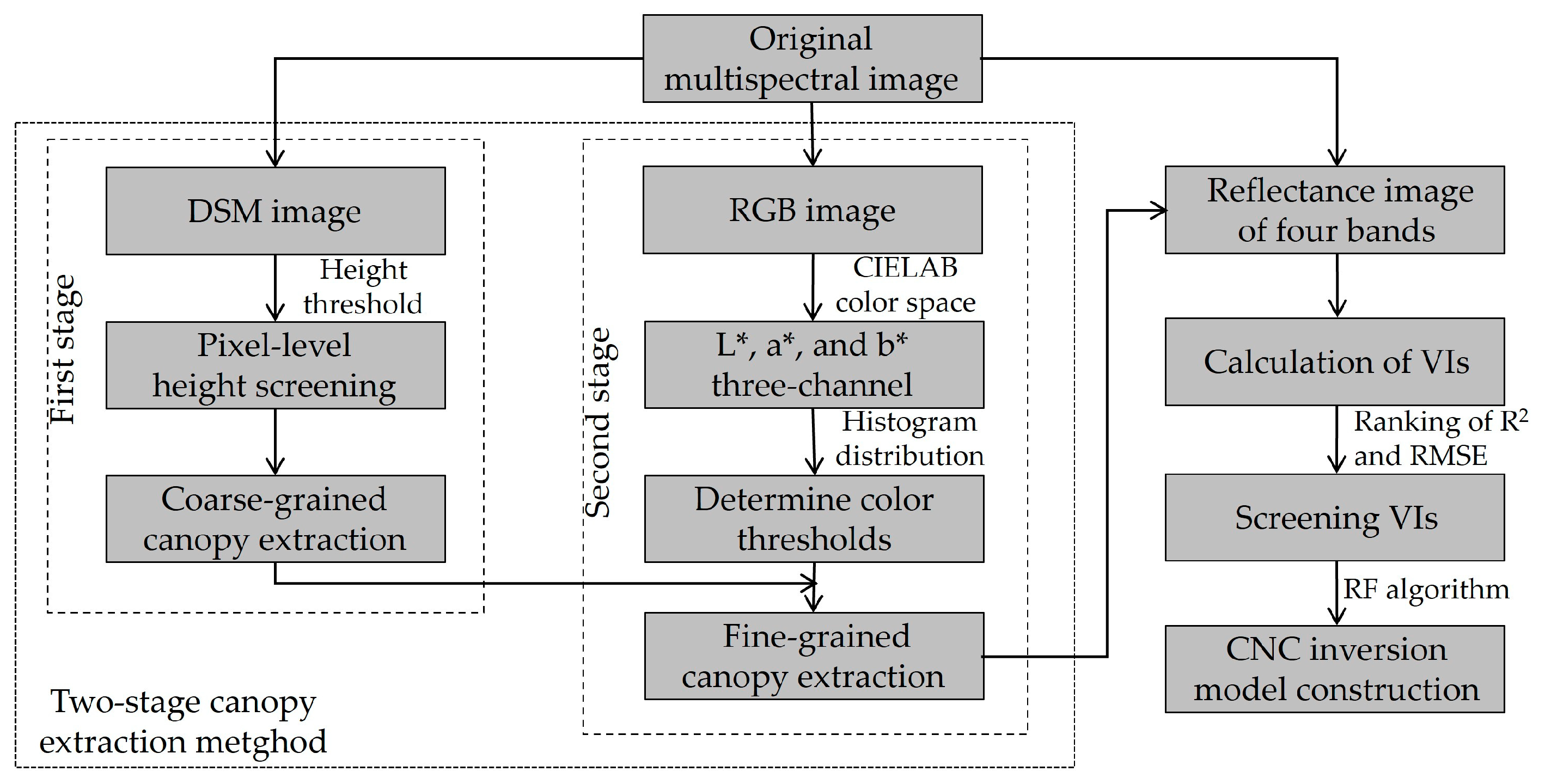
The overall technical road map is illustrated in Figure 4. Firstly, the DSM image of the original multispectral image was used to realize pixel-level height screening based on the set height threshold; thereby, the coarse-grained canopy was extracted. Then, the RGB image of the original multispectral image was converted into the following three channels: L*, a*, and b*. The color thresholds were determined based on the histogram distribution of the three-channel values. According to the determined color thresholds, the extracted coarse-grained canopy was further processed, thereby obtaining the fine-grained canopy. Finally, VIs can be calculated based on the extracted canopy reflectance of the four bands. According to the ranking of R2 and RMSE, the suitable VIs were selected to construct the CNC inversion model using the RF algorithm.

3. Results

3.1. Determination of Color Thresholds

To explain how color thresholds were determined, histograms were utilized to statistically analyze the data distribution of the L*, a*, and b* channels. Figure 5 contains a pear tree in the JAAS orchard as an example and shows the data distribution of the three-channel values (L*, a*, and b*) after the height difference processing of the first stage. It can be concluded that the three-channel values of L*, a*, and b* all approximately exhibited normal distributions. The normal distribution curves (red lines) of the L*, a*, and b* channels were fitted based on the distribution of the three-channel values. The parameters of the fitted curves, including the mean value (μ) and standard deviation (σ), are summarized in Table 4.
In statistics, the confidence interval is usually used to indicate the reliability of estimated values and the error range [48,49]. The values outside the interval are usually regarded as error values. As for the screening of the L*, a*, and b* three-channel values, the interference factors can also be regarded as error values. For example, shadows are the lower values in the L* channel. Thus, in this paper, the confidence level of the confidence interval was used to determine the color thresholds of the L*, a*, and b* channels. Generally, the confidence level is set at 95%. Furthermore, according to the parameters of the fitted normal distribution curves, the lower and upper limit thresholds of the L*, a*, and b* channels can be calculated by μ − 2σ and μ + 2σ, respectively, as shown in Table 4. In this example, the value of the L* channel ranged from 23.626 to 67.718. The value of the a* channel ranged from −31.433 to −7.977. The value of the b* channel ranged from 2.201 to 27.313. A pixel was considered an invalid pixel and eliminated if the value of any channel did not meet the requirements of the threshold range.
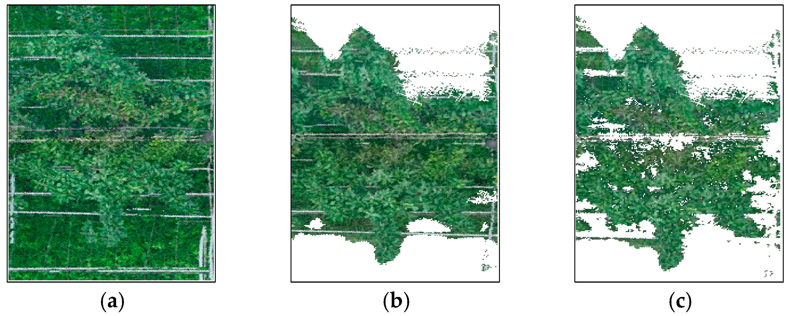
Figure 6 shows an example of two-stage canopy extraction in the JAAS orchard. Firstly, based on the original RGB image (Figure 6a), the coarse-grained canopy (Figure 6b) can be extracted by eliminating the surficial grass, using the height difference. Then, based on the coarse-grained canopy extraction result, the fine-grained canopy extraction can be achieved by eliminating the shadows, branches, and trellis using the color thresholds of the L*, a*, and b* channels.

3.2. Results of Canopy Extraction

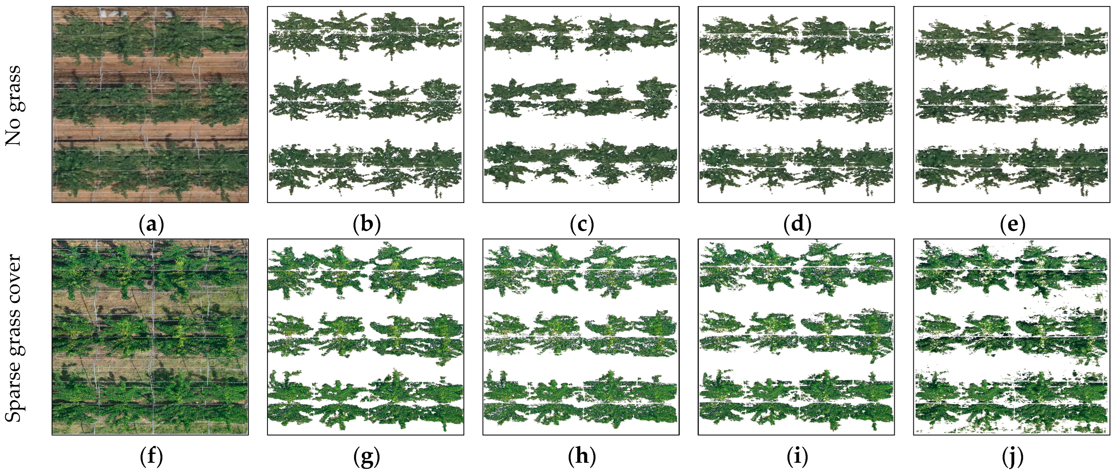
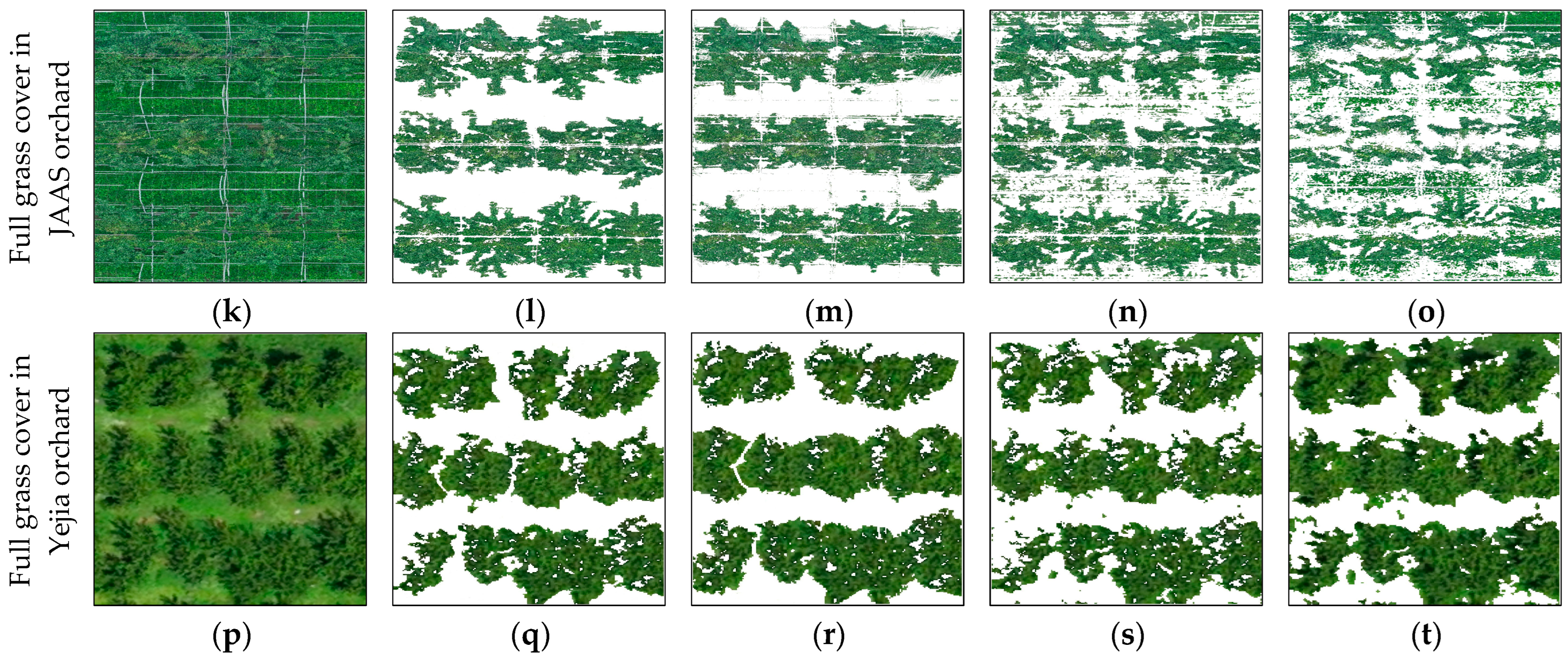
To better illustrate the performance of our proposed methods for canopy extraction, three baseline methods were adopted for comparative analysis through extracting canopies in four scenarios, as shown in Figure 7. Table 5 shows the accuracy evaluation indicators of canopy extraction among three methods, i.e., TCE, TFS, and ITE. In this section, visualized canopy extraction figures and quantified experimental results were utilized to comprehensively analyze the performance of canopy extraction for each method. It is worth noting that Figure 7b,g,l,q present the canopy extraction results of the MPF. This method was taken as a benchmark extraction approach to compare the extraction effects and calculate the accuracy metrics for canopy extraction.
As shown in Figure 7c–e, in the scenario without grass, all of the TCE, TFS, and ITE can effectively achieve the goal of canopy extraction. The experimental results show that the extraction accuracy metrics of the three methods were all better than 90%, and the ranking of accuracy was TFS > ITE > TCE. As shown in Figure 7h–j, in the scenario with sparse grass cover, TCE and TFS can still effectively extract the canopies of pear trees. However, in the extracted canopies of ITE, some grassy areas were not completely removed, thereby leading to slight decreases in extraction accuracy metrics. Generally, the extraction accuracy metrics of the three methods were still better than 90%. As shown in Figure 7m–o, in the scenario with full grass cover in the JAAS orchard, the extracted canopies of TFS and ITE contained a large number of grassy areas. In other words, the ratio of FN pixels increased, thereby leading to significant declines in the extraction accuracy metrics of these two methods. For example, the accuracy, recall, precision, and F1-score of the ITE were 73.205%, 80.091%, 78.216%, and 79.142%, respectively. In contrast, TCE still demonstrated favorable effects in canopy extraction. All of its extraction accuracy metrics exceeded 90%. Figure 7r–t present similar results to those in Figure 7m–o. All the extraction accuracy metrics of TCE were the best and exceeded 90%. Although the extraction accuracy metrics of TFS and ITE in the Yejia orchard were better than those in the JAAS orchard, their metrics were still worse than those of TCE. The above results proved that our proposed method can effectively address the problem of canopy extraction in scenarios with full grass cover and has good robustness and generalization in different scenarios.

3.3. Result of VI Screening

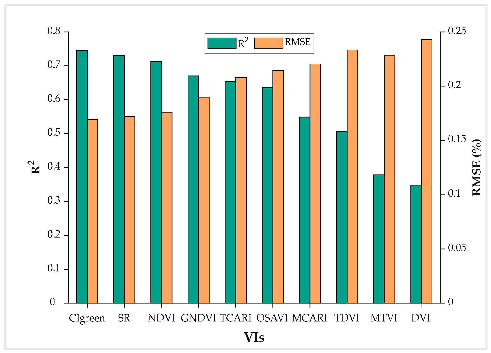
Figure 8 shows that 10 VIs were ranked according to the magnitude of R2 and RMSE. The values of R2 and RMSE are listed in Table 6. It is worth noting that in this section, the VIs were calculated based on the extracted canopy reflectance of the MPF. It can be found that VIs with higher R2 values also had lower RMSE values. Theoretically, the higher the ranking of the VIs, the better the estimation accuracy that can be achieved for CNC inversion. Therefore, three top VIs were screened for constructing CNC inversion models. The screened VIs included the CIgreen, SR, and NDVI.

3.4. Comparison of CNC Inversion Models

To illustrate the estimation accuracy of the constructed CNC inversion models based on our proposed canopy extraction method, we utilized the top three VIs, which were screened in Section 3.3, to construct CNC inversion models in the four scenarios. As shown in Figure 9, in the scenario with no grass, for the top three VIs, the ranking of the accuracy metrics of the constructed CNC inversion models was consistent with the screened ranking (CIgreen > SR > NDVI). MPF, as the benchmark extraction approach, demonstrated the optimal modeling performance, featuring the highest R2 and the lowest RMSE and nRMSE in each of the constructed models.
In the scenario with sparse grass cover, as shown in Figure 10, using MPF to extract canopies constructed the best CNC inversion model (R2 = 0.794, RMSE = 0.227, and nRMSE = 13.187%). Although the estimation accuracy metrics of the constructed CNC inversion models based on TFS and ITE were good in the scenarios with no grass or sparse grass cover, they were poor in the scenarios with full grass cover.
Using ITE to extract canopies constructed the worst CIgreen-based CNC inversion model (R2 = 0.649, RMSE = 0.378, and nRMSE = 29.742%) in the scenario with full grass cover in the JAAS orchard, as shown in Figure 11. The estimation accuracy metrics of this model fail to meet the requirements of practical applications. Unlike these two methods, TCE exhibited good modeling effects for CNC inversion in all four scenarios.
As shown in Figure 12, when using TCE to extract canopies in the scenarios with full grass cover in the Yejia orchard, the values of R2 were higher than 0.744, and the RMSE and nRMSE were lower than 0.243 and 15.955%, respectively. Furthermore, in the scenarios with full grass cover, the estimation accuracy metrics of the TCE-based CNC inversion models were all superior to those of the TFS and ITE-based CNC inversion models. The above results prove that our proposed method can improve the estimation accuracy of the CNC inversion model in the scenarios with full grass cover. In the scenarios with no grass or sparse grass cover, our proposed method also has good modeling performance for CNC inversion.

3.5. Spatial Inversion Mapping of CNC

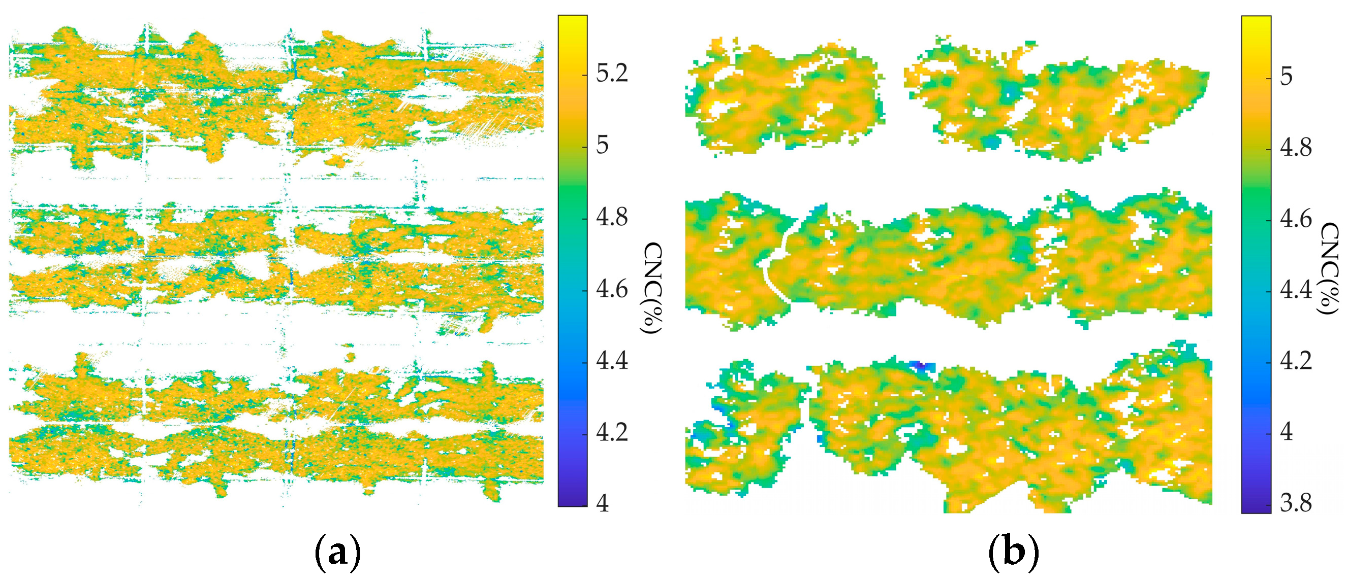
To better observe the distribution of CNC in pear orchards, heat maps were used to present the pixel-level nitrogen content. Figure 13a,b display the CNC inversion maps in partial regions of the JAAS pear orchard and the Yejia pear orchard, respectively. In these two displayed areas, it can be observed that the distribution of CNC was relatively similar. The CNC ranged from 4.007 to 5.278 in the JAAS pear orchard and from 3.785 to 5.182 in the Yejia pear orchard. The reasons may be that the pear trees in these two orchards were in the same phenological period due to the similar climatic conditions in these two areas and the close data collection time. Although similar, the CNC values reported for the two orchards are not identical. This could be caused by the different fertilizer application and water management techniques applied. The JAAS orchard had solid fertilizer and drip irrigation to manage the application of fertilizer and water. However, the Yejia orchard had liquid organic fertilizer, e.g., the biogas slurry, after fermentation, to supplement fertilizer and water simultaneously.

4. Discussion

This paper explored the feasibility of using the TCE method to address the canopy extraction problem in the scenario of full grass cover. We found that TCE can accurately extract canopies in different scenarios. Moreover, the constructed CNC inversion models, which use TCE to extract canopies, had a high R2 and low RMSE and nRMSE, and they can improve the spatial inversion of CNC in the scenario of full grass cover.

4.1. Analysis of Coarse-Grained Canopy Extraction Based on Height Difference

Previous studies mainly focused on the scenarios with no grass or sparse grass cover and paid less attention to the scenario with full grass cover in pear orchards. The existing IT [16] and TC-based [17] canopy extraction methods, as the most commonly used methods, can solve the canopy extraction problem in the scenarios with no grass or sparse grass cover. Thus, the height difference between the canopies of fruit trees and ground grass was rarely used to extract the canopies of fruit trees. However, as shown in Figure 7n,s,o,t, in the scenarios with full grass cover, IT and TC-based canopy extraction methods cannot meet the requirement of accurate canopy extraction. The extraction accuracy metrics of these two methods decreased significantly. One of the important reasons is that the ratio of FN increased. In other words, a large number of pixels belonging to grass were classified into the canopy area. Although adopting supervised machine learning or deep learning [50,51] could improve the extraction accuracy metrics of TC-based canopy extraction methods, they are labor-intensive. Meanwhile, precisely labeling the grass coverage area and the canopy area is challenging, as shown in Figure 7k. Thus, it is particularly important to preprocess the original RGB images using the height difference. The results in Figure 7m,r all demonstrate this point.
Furthermore, it is worth noting that there are also some challenges in using the height difference to extract the canopies of pear trees. Firstly, the accuracy of elevation information directly affects the accuracy of canopy extraction. Due to the complexity of the orchard environment, uncontrollable gusts of wind would cause the UAV and branches to sway, thereby affecting the accuracy of elevation information in shaking areas. This situation could explain why the canopies extracted based on TCE had the problem of disappearing branch tips. By consulting the manufacturer, we learned that increasing the overlap rate, e.g., a side overlap rate of 75% and a course overlap rate of 85%, of the collected images is a feasible solution. Secondly, the setting of the difference threshold should be self-adapting. In this paper, the two orchards are located in areas with gentle terrain, and meanwhile, the growth differences of pear trees are not significant. Thus, a uniform height threshold was adopted. However, there are many orchards located in hilly and sloping areas [52]. A uniform height threshold setting is clearly not applicable. Thus, it is necessary to study the self-adapting settings of height thresholds.

4.2. Analysis of Fine-Grained Canopy Extraction Based on Color Thresholds

Based on the extracted coarse-grained canopies, interfering factors in canopies, e.g., branches, trellis, and shadows, need to be further eliminated to enhance the estimation accuracy of constructed CNC inversion models. Theoretically, both IT and TC-based canopy extraction methods can be used to extract fine-grained canopies. For the IT-based canopy extraction method, although this method would have a good effect on removing branches and trellis due to the significant differences in VI values, it cannot effectively eliminate shadow areas. Generally, the VI values in shaded areas are lower than those in illuminated areas. However, some previous studies have also shown that the VI values of the parts with lower CNC in the illuminated areas and the parts with higher CNC in the shadow areas are very close [16], which poses a challenge to the setting of the screening thresholds. The results in Figure 7j,t also proved this conclusion. For the TC-based canopy extraction method, supervised learning could be a good choice to ensure extraction accuracy. Nevertheless, considering the labor-intensive labeling work, this method is not the preferred opinion in this paper.
Based on the above reasons, in this paper, we utilized the characteristics of the CIELAB color space to achieve the fine-grained canopy extraction. The characteristics are as follows: adjusting the lightness values (L* channel) of pixels will not change their color values, and adjusting the color values of pixels will not change their lightness values, either [53]. This is the main basis for eliminating the shaded areas from the extracted coarse-grained canopies. The histograms in Figure 5 well illustrate the data distribution of the L*, a*, and b* channels. Determining the color thresholds by fitting the normal distribution curves and calculating the upper and lower limit thresholds of the confidence interval can meet the requirements of statistical theory and is scientific. Due to the visibility of colors, with the assistance of the CIELAB color space, a better interpretation of the screening of canopy pixels can be achieved. All the experimental results demonstrate the feasibility of this method.

4.3. Construction of CNC Inversion Model and Visualization of CNC Distribution

The core research content of this paper is to improve the estimation accuracy of CNC inversion in the scenario with full grass cover. This section mainly focuses on analyzing the influence of the canopy extraction effects on the estimation accuracy of the constructed CNC inversion models. By comparing Table 5 and Figure 9, it can be found that the more precise the extracted canopy is, the higher the estimation accuracy of the constructed inversion model will be. This conclusion is applicable to various methods and scenarios. For TCE, the estimation accuracy, i.e., R2, RMSE, and nRMSE, of its CNC inversion models changed slightly in four scenarios. However, in the scenario of full grass cover, due to the significant decline in canopy extraction accuracy, the estimation accuracy of the CNC inversion models for TFS and ITE also decreased significantly. This result demonstrates that accurate canopy extraction is the crucial condition for achieving a high estimation accuracy of CNC inversion [16].
Furthermore, through observing the color changes in the canopies in Figure 10, we found that the CNC at the top of the canopy is usually higher than that at the bottom. This conclusion was consistent with the existing studies [2] and indicated the heterogeneity of the longitudinal distribution of nitrogen in the canopy [54]. The visualization of the CNC distribution can also offer technical support for pear orchard managers, helping them better understand the growth of pear trees and adopt reasonable strategies for nitrogen fertilizer application.

4.4. Performance Comparison of Canopy Extraction and CNC Inversion Based on TCE in the Two Orchards

This paper selected two orchards, the JAAS orchard and the Yejia orchard, to verify the feasibility of the TCE. In this section, the performances of canopy extraction and CNC inversion based on TCE in the two orchards were compared to reveal the possible differences when the TCE is used in different orchards.
Overall, whether it is canopy extraction or the construction of CNC inversion models, the key accuracy evaluation indicators in the Yejia orchard are better than those in the JAAS orchard. For example, the precision of canopy extraction and the R2 value of the CIgreen-based CNC inversion model in the Yejia orchard are 93.392% and 0.744, respectively, and these values are superior to those (precision = 91.284, R2 = 0.724) in the JAAS orchard.
On one hand, the accuracy of canopy extraction could be influenced by the quality of the collected original spectral images, especially the quality of DSM data. This accuracy would further affect the estimation accuracy of CNC inversion [16]. On the other hand, different water and fertilizer management could cause differences in the canopy structures of pear trees. For example, applying liquid organic fertilizer in the Yejia orchard could facilitate the nutrient absorption of pear trees, thereby forming a higher-degree canopy density and affecting the propagation of sunlight in the canopy. Thus, this situation would also influence the accuracy of canopy extraction and CNC inversion.

4.5. Future Prospects and Challenges

In this section, the future prospects and challenges are summarized. Firstly, this paper successfully extracted the canopies of pear trees in the scenarios with full grass cover. The pixel-level data processing based on the traversing method is the key to achieving highly accurate canopy extraction. However, this method would consume a large amount of computing resources and have low processing efficiency. How to balance the accuracy and processing efficiency needs to be considered when our proposed method is applied in a larger orchard.
Secondly, in this paper, the positioning of fruit trees and the division of their sub-regions were achieved through manual calibration. Fusing some advanced artificial intelligence technologies to achieve the location and sub-regions division of pear trees would greatly enhance the efficiency of data preprocessing.
Thirdly, in some orchard scenarios of hilly and mountainous areas, an adaptive selection strategy for height thresholds should be designed to enhance the accuracy of coarse-grained canopy extraction.

5. Conclusions

Accurate canopy extraction is crucial for improving the estimation accuracy of CNC inversion. This study proposed a two-stage canopy extraction method to address the issue of canopy extraction in the scenario with full grass cover. In this study, firstly, the height difference between the canopies of pear trees and the ground grass was used to eliminate the interference of the ground grass and achieve the coarse-grained canopy extractions. Then, based on the extracted coarse-grained canopies, the data distribution of L*, a*, and b* from the histogram and the thresholds of the confidence interval were used to determine the color thresholds of the three channels to complete the fine-grained canopy extraction. Thirdly, the RF algorithm was used to select suitable VIs based on the R2 and RMSE values and then construct CNC inversion models. Finally, all the experiments on canopy extraction and CNC inversion model construction exhibited that TCE, our proposed method, can effectively extract the canopies in the four set scenarios and achieve a high estimation accuracy of CNC inversion. Thus, our proposed method can provide technical support for the efficient and non-destructive monitoring of the canopy nutrient status in pear orchards.

Author Contributions

Conceptualization, Y.S. and X.L. (Xiaolan Lv); methodology, Y.S. and K.H.; software, Y.S.; validation, K.H., Q.Y. and X.L. (Xiaohui Lei); data curation, Y.S. and K.H.; writing—original draft preparation, Y.S.; writing—review and editing, K.H., Q.Y. and X.L. (Xiaohui Lei); supervision and funding acquisition, X.L. (Xiaolan Lv). All authors have read and agreed to the published version of the manuscript.

Funding

This study was funded in part by the Jiangsu Funding Program for Excellent Postdoctoral Talent (JB24090), the China Agriculture Research System of MOF and MARA (CARS-28-21), and the Jiangsu Province Agricultural Machinery Research and Development, Manufacturing, Promotion and Application Integrated Pilot Project (JSYTH01).

Data Availability Statement

The data presented in this study are available on request from the corresponding author due to privacy for ongoing research.

Acknowledgments

We would like to thank the kind help of all the editors and the reviewers to improve the manuscript.

Conflicts of Interest

The authors declare no conflicts of interest.

References

  1. Li, H.; Zhang, J.; Xu, K.; Jiang, X.; Zhu, Y.; Cao, W.; Ni, J. Spectral monitoring of wheat leaf nitrogen content based on canopy structure information compensation. Comput. Electron. Agric. 2021, 190, 106434. [Google Scholar] [CrossRef]
  2. Zhang, C.; Zhu, X.; Li, M.; Xue, Y.; Qin, A.; Gao, G.; Wang, M.; Jiang, Y. Utilization of the fusion of ground-space remote sensing data for canopy nitrogen content inversion in apple orchards. Horticulturae 2023, 9, 1085. [Google Scholar] [CrossRef]
  3. Saez-Plaza, P.; Navas, M.J.; Wybraniec, S.; Michalowski, T.; Asuero, A.G. An Overview of the Kjeldahl Method of Nitrogen Determination. Part II. Sample Preparation, Working Scale, Instrumental Finish, and Quality Control. Crit. Rev. Anal. Chem. 2013, 43, 224–272. [Google Scholar] [CrossRef]
  4. Avioz, D.; Linker, R.; Raveh, E.; Baram, S.; Paz-Kagan, T. Multi-scale remote sensing for sustainable citrus farming: Predicting canopy nitrogen content using UAV-satellite data fusion. Smart. Agric. Technol. 2025, 11, 100906. [Google Scholar] [CrossRef]
  5. Wang, L.; Chen, S.; Peng, Z.; Huang, J.; Wang, C.; Jiang, H.; Zheng, Q.; Li, D. Phenology effects on physically based estimation of paddy rice canopy traits from UAV hyperspectral imagery. Remote Sens. 2021, 13, 1792. [Google Scholar] [CrossRef]
  6. Liao, Z.; Dai, Y.; Wang, H.; Ketterings, Q.; Lu, J.; Zhang, F.; Li, Z.; Fan, J. A doublelayer model for improving the estimation of wheat canopy nitrogen content from unmanned aerial vehicle multispectral imagery. J. Integr. Agric. 2023, 22, 2248–2270. [Google Scholar] [CrossRef]
  7. Tang, Y.; Li, F.; Hu, Y.; Yu, K. Exploring the optimal wavelet function and wavelet feature for estimating maize leaf chlorophyll content. IEEE Trans. Geosci. Remote Sens. 2025, 63, 4400812. [Google Scholar] [CrossRef]
  8. Azadnia, R.; Rajabipour, A.; Jamshidi, B.; Omid, M. New approach for rapid estimation of leaf nitrogen, phosphorus, and potassium contents in apple-trees using Vis/NIR spectroscopy based on wavelength selection coupled with machine learning. Comput. Electron. Agric. 2023, 207, 107746. [Google Scholar] [CrossRef]
  9. Hasan, U.; Jia, K.; Wang, L.; Wang, C.; Shen, Z.; Yu, W.; Sun, Y.; Jiang, H.; Zhang, Z.; Guo, J.; et al. Retrieval of leaf chlorophyll contents (LCCs) in litchi based on fractional order derivatives and VCPA-GA-ML algorithms. Plants 2023, 12, 501. [Google Scholar] [CrossRef]
  10. Kong, W.; Ma, L.; Ye, H.; Wang, J.; Nie, C.; Chen, B.; Zhou, X.; Huang, W.; Fan, Z. Nondestructive estimation of leaf chlorophyll content in banana based on unmanned aerial vehicle hyperspectral images using image feature combination methods. Front. Plant Sci. 2025, 16, 1536177. [Google Scholar] [CrossRef]
  11. Dong, X.; Zhang, Z.; Yu, R.; Tian, Q.; Zhu, X. Extraction of information about individual trees from high-spatial-resolution UAV-acquired images of an orchard. Remote Sens. 2020, 12, 133. [Google Scholar] [CrossRef]
  12. Cheng, Z.; Qi, L.; Cheng, Y. Cherry tree crown extraction from natural orchard images with complex backgrounds. Agriculture 2021, 11, 431. [Google Scholar] [CrossRef]
  13. Lu, Z.; Qi, L.; Zhang, H.; Wan, J.; Zhou, J. Image segmentation of UAV fruit tree canopy in a natural illumination environment. Agriculture 2022, 12, 1039. [Google Scholar] [CrossRef]
  14. Zhang, C.; Chen, Z.; Yang, G.; Xu, B.; Feng, H.; Chen, R.; Qi, N.; Zhang, W.; Zhao, D.; Cheng, J.; et al. Removal of canopy shadows improved retrieval accuracy of individual apple tree crowns LAI and chlorophyll content using UAV multispectral imagery and PROSAIL model. Comput. Electron. Agric. 2024, 221, 108959. [Google Scholar] [CrossRef]
  15. Li, Z.; Deng, X.; Lan, Y.; Liu, C.; Qing, J. Fruit tree canopy segmentation from UAV orthophoto maps based on a lightweight improved U-Net. Comput. Electron. Agric. 2024, 217, 108538. [Google Scholar] [CrossRef]
  16. Wei, P.; Yan, X.; Yan, W.; Sun, L.; Xu, J.; Yuan, H. Precise extraction of targeted apple tree canopy with YOLO-Fi model for advanced UAV spraying plans. Comput. Electron. Agric. 2024, 226, 109425. [Google Scholar] [CrossRef]
  17. Wang, L.; Zhang, R.; Zhang, L.; Yi, T.; Zhang, D.; Zhu, A. Research on individual tree canopy segmentation of Camellia oleifera based on a UAV-LiDAR system. Agriculture 2024, 14, 364. [Google Scholar] [CrossRef]
  18. Yang, Y.; Zeng, T.; Li, L.; Fang, J.; Fu, W.; Gu, Y. Canopy extraction of mango trees in hilly and plain orchards using UAV images: Performance of machine learning vs deep learning. Ecol. Inform. 2025, 87, 103101. [Google Scholar] [CrossRef]
  19. Chen, L.; Bao, Y.; He, X.; Yang, J.; Wu, Q.; Lv, J. Nature-based accumulation of organic carbon and nitrogen in citrus orchard soil with grass coverage. Soil. Till. Res. 2025, 248, 106419. [Google Scholar] [CrossRef]
  20. Wang, Z.; Liu, R.; Fu, L.; Tao, S.; Bao, J. Effects of orchard grass on soil fertility and nutritional status of fruit trees in Korla fragrant pear orchard. Horticulturae 2023, 9, 903. [Google Scholar] [CrossRef]
  21. Wang, A.; Zhang, W.; Wei, X. A review on weed detection using ground-based machine vision and image processing techniques. Comput. Electron. Agric. 2019, 158, 226–240. [Google Scholar] [CrossRef]
  22. Gong, Y.; Liu, G.; Xue, Y.; Li, R.; Meng, L. A survey on dataset quality in machine learning. Inform. Software. Tech. 2023, 162, 107268. [Google Scholar] [CrossRef]
  23. Shen, W.; Peng, Z.; Wang, X.; Wang, H.; Cen, J.; Jiang, D.; Xie, L.; Yang, X.; Tian, Q. A survey on label-efficient deep image segmentation: Bridging the gap between weak supervision and dense prediction. IEEE Trans. Pattern. Anal. Mach. Intell. 2023, 45, 9284–9305. [Google Scholar] [CrossRef]
  24. Polat, N.; Memduhoğlu, A.; Kaya, Y. Accurate Terrain Modeling After Dark: Evaluating Nighttime Thermal UAV-Derived DSMs. Drones 2025, 9, 430. [Google Scholar] [CrossRef]
  25. Xi, R.; Gu, Y.; Zhang, X.; Ren, Z. Nitrogen monitoring and inversion algorithms of fruit trees based on spectral remote sensing: A deep review. Front. Plant. Sci. 2024, 15, 1489151. [Google Scholar] [CrossRef]
  26. Wrat, G.; Ranjan, P.; Mishra, S.K.; Jose, J.T.; Das, J. Neural network-enhanced internal leakage analysis for efficient fault detection in heavy machinery hydraulic actuator cylinders. Proc. Inst. Mech. Eng. Part C J. Mech. Eng. Sci. 2025, 239, 1021–1031. [Google Scholar] [CrossRef]
  27. Li, W.; Zhu, X.; Yu, X.; Li, M.; Tang, X.; Zhang, J.; Xue, Y.; Zhang, C.; Jiang, Y. Inversion of nitrogen concentration in apple canopy based on UAV hyperspectral images. Sensors 2022, 22, 3503. [Google Scholar] [CrossRef]
  28. Li, M.X.; Zhu, X.C.; Li, W.; Tang, X.Y.; Yu, X.Y.; Jiang, Y.M. Retrieval of Nitrogen Content in Apple Canopy Based on Unmanned Aerial Vehicle Hyperspectral Images Using a Modified Correlation Coefficient Method. Sustainability 2022, 14, 1992. [Google Scholar] [CrossRef]
  29. Jia, Y.; Li, Y.; He, J.; Biswas, A.; Siddique, K.H.; Hou, Z.; Luo, H.; Wang, C.; Xie, X. Enhancing precision nitrogen management for cotton cultivation in arid environments using remote sensing techniques. Field. Crop. Res. 2025, 321, 109689. [Google Scholar]
  30. Donmez, C.; Villi, O.; Berberoglu, S.; Cilek, A. Computer vision-based citrus tree detection in a cultivated environment using UAV imagery. Comput. Electron. Agric. 2021, 187, 106273. [Google Scholar] [CrossRef]
  31. Din, M.; Zheng, W.; Rashid, M.; Wang, S.; Shi, Z. Evaluating hyperspectral vegetation indices for leaf area index estimation of Oryza sativa L. at diverse phenological stages. Front. Plant. Sci. 2017, 8, 820. [Google Scholar]
  32. Cheng, J.; Yang, H.; Qi, J.; Sun, Z.; Han, S.; Feng, H.; Jiang, J.; Xu, W.; Li, Z.; Yang, G.; et al. Estimating canopy-scale chlorophyll content in apple orchards using a 3D radiative transfer model and UAV multispectral imagery. Comput. Electron. Agric. 2022, 202, 107401. [Google Scholar] [CrossRef]
  33. Gribble, C.; Ize, T.; Kensler, A.; Wald, I.; Parker, S. A coherent grid traversal approach to visualizing particle-based simulation data. IEEE Trans. Vis. Comput. Graph. 2007, 13, 758–768. [Google Scholar] [CrossRef]
  34. Lillotte, T.; Joester, M.; Frindt, B.; Berghaus, A.; Lammens, R.F.; Wagner, K.G. UV–VIS spectra as potential process analytical technology (PAT) for measuring the density of compressed materials: Evaluation of the CIELAB color space. Int. J. Pharmaceut. 2021, 603, 120668. [Google Scholar]
  35. Zhang, Y.; Li, X.; Wang, M.; Xu, T.; Huang, K.; Sun, Y.; Yuan, Q.; Lei, X.; Qi, Y.; Lv, X. Early detection and lesion visualization of pear leaf anthracnose based on multi-source feature fusion of hyperspectral imaging. Front. Plant Sci. 2024, 15, 1461855. [Google Scholar] [CrossRef] [PubMed]
  36. Sabha, M.; Saffarini, M. Selecting optimal k for K-means in image segmentation using GLCM. Multimed. Tools. Appl. 2024, 83, 55587–55603. [Google Scholar]
  37. Zhao, Z.; Lu, C.; Tonooka, H.; Wu, L.; Lin, H.; Jiang, X. Dynamic monitoring of vegetation phenology on the Qinghai-Tibetan plateau from 2001 to 2020 via the MSAVI and EVI. Sci. Rep. 2025, 15, 25698. [Google Scholar] [CrossRef]
  38. Rouse, J. Monitoring vegetation systems in the great plains with ERTS. In Third NASA Earth Resources Technology Satellite Symposium; NASA: Washington, DC, USA, 1973; Volume 1, pp. 309–317. [Google Scholar]
  39. Rondeaux, G.; Steven, M.; Baret, F. Optimization of soil-adjusted vegetation indices. Remote. Sens. Environ. 1996, 55, 95–107. [Google Scholar] [CrossRef]
  40. Roujean, J.-L.; Breon, F.-M. Estimating PAR absorbed by vegetation from bidirectional reflectance measurements. Remote Sens. Environ. 1995, 51, 375–384. [Google Scholar]
  41. Gitelson, A.; Kaufman, Y.; Merzlyak, M. Use of a green channel in remote sensing of global vegetation from EOS-MODIS. Remote Sens. Environ. 1996, 58, 289–298. [Google Scholar]
  42. Carter, G. Ratios of leaf reflectances in narrow wavebands as indicators of plant stress. Remote Sens. 1994, 15, 697–703. [Google Scholar] [CrossRef]
  43. Gitelson, A.; Gritz, Y.; Merzlyak, M. Relationships between leaf chlorophyll content and spectral reflectance and algorithms for non-destructive chlorophyll assessment in higher plant leaves. Plant Physiol. 2003, 160, 271–282. [Google Scholar] [CrossRef] [PubMed]
  44. Daughtry, C.; Walthall, C.; Kim, M.; De Colstoun, E.; McMurtrey, I. Estimating corn leaf chlorophyll concentration from leaf and canopy reflectance. Remote Sens. Environ. 2000, 74, 229–239. [Google Scholar] [CrossRef]
  45. De Grave, C.; Verrelst, J.; Morcillo-Pallarés, P.; Pipia, L.; Rivera-Caicedo, J.P.; Amin, E.; Belda, S.; Moreno, J. Quantifying vegetation biophysical variables from the Sentinel-3/FLEX tandem mission: Evaluation of the synergy of OLCI and FLORIS data sources. Remote Sens. Environ. 2020, 251, 112101. [Google Scholar] [CrossRef]
  46. Darvishzadeh, R.; Skidmore, A.; Schlerf, M.; Atzberger, C. Inversion of a radiative transfer model for estimating vegetation LAI and chlorophyll in a heterogeneous grassland. Remote Sens. Environ. 2008, 112, 2592–2604. [Google Scholar] [CrossRef]
  47. Haboudane, D.; Miller, J.; Pattey, E.; Zarco-Tejada, P.; Strachan, I. Hyperspectral vegetation indices and novel algorithms for predicting green LAI of crop canopies: Modeling and validation in the context of precision agriculture. Remote Sens. Rev. 2004, 90, 337–352. [Google Scholar] [CrossRef]
  48. Hosmer, D.; Lemeshow, S. Confidence interval estimation of interaction. Epidemiology 1992, 3, 452–456. [Google Scholar] [CrossRef]
  49. Shi, C.; Zhu, J.; Shen, Y.; Luo, S.; Zhu, H.; Song, R. Off-policy confidence interval estimation with confounded markov decision process. J. Am. Stat. Assoc. 2024, 119, 273–284. [Google Scholar] [CrossRef]
  50. Rao, L.; Yuan, Y.; Shen, X.; Yu, G.; Chen, X. Designing nanotheranostics with machine learning. Nat. Nanotechnol. 2024, 19, 1769–1781. [Google Scholar] [CrossRef] [PubMed]
  51. Mienye, I.; Swart, T. A comprehensive review of deep learning: Architectures, recent advances, and applications. Information 2024, 15, 755. [Google Scholar] [CrossRef]
  52. Chen, P.; Liu, S.; Xu, J.; Liu, M. Stability control of a wheel-legged mobile platform used in hilly orchards. Biosyst. Eng. 2025, 256, 104195. [Google Scholar] [CrossRef]
  53. Malounas, I.; Lentzou, D.; Xanthopoulos, G.; Fountas, S. Testing the suitability of automated machine learning, hyperspectral imaging and CIELAB color space for proximal in situ fertilization level classification. Smart Agric. Technol. 2024, 8, 100437. [Google Scholar] [CrossRef]
  54. Wang, B.; Gu, S.; Wang, J.; Chen, B.; Wen, W.; Guo, X.; Zhao, C. Maximizing the radiation use efficiency by matching the leaf area and leaf nitrogen vertical distributions in a maize canopy: A simulation study. Plant Phenomics 2024, 6, 0217. [Google Scholar] [CrossRef] [PubMed]
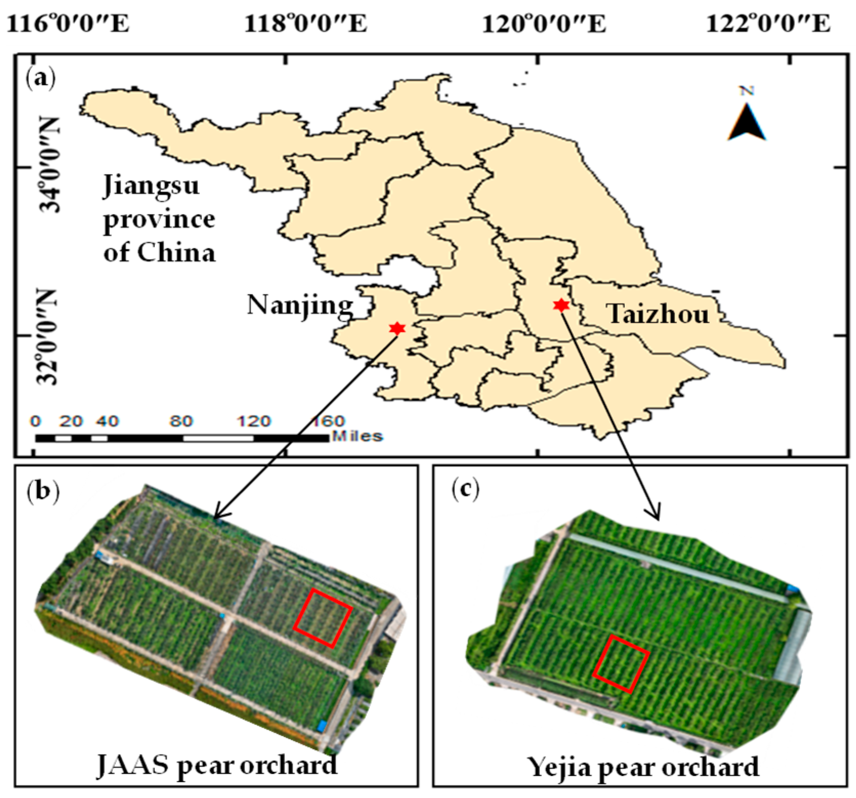
Figure 1. Description of the study area. (a) Location of the two orchards. (b) A UAV image of JAAS pear orchard. (c) A UAV image of Yejia pear orchard. Red outlines were used to visualize the experimental results.
Horticulturae 11 01419 g001
Figure 2. Examples of images in three classic typical scenarios. (a) No grass. (b) Sparse grass cover. (c) Full grass cover.
Horticulturae 11 01419 g002
Figure 3. Elevation distribution in scenario with full grass cover. (a) Original image. (b) Elevation information map.
Horticulturae 11 01419 g003
Figure 4. Technology road map.
Horticulturae 11 01419 g004
Figure 5. Histogram distribution of L*, a*, and b* three-channel values through the height difference processing of the first stage. (a) Frequency of pixel values occurred in L* channel; (b) frequency of pixel values occurred in a* channel; (c) frequency of pixel values occurred in b* channel.
Horticulturae 11 01419 g005
Figure 6. An example of two-stage canopy extraction. (a) Original RGB image of single pear tree. (b) Coarse-grained canopy extraction based on height difference. (c) Fine-grained canopy extraction based on color thresholds.
Horticulturae 11 01419 g006
Figure 7. Canopy extraction results based on RGB images for four methods in four scenarios. (a,f,k,p): Original images of four scenarios. (b,g,l,q): Canopy extraction results of MPF in four scenarios. (c,h,m,r): Canopy extraction results of TCE (our proposed method) in four scenarios. (d,i,n,s): Canopy extraction results of TFS in four scenarios. (e,j,o,t): Canopy extraction results of ITE in four scenarios.
Horticulturae 11 01419 g007aHorticulturae 11 01419 g007b
Figure 8. Screening of VIs based on ranking of R2 and RMSE.
Horticulturae 11 01419 g008
Figure 9. Performance comparison of CNC inversion models in the scenario with no grass. (a) CIgreen-based; (b) SR-based; (c) NDVI-based.
Horticulturae 11 01419 g009
Figure 10. Performance comparison of CNC inversion models in the scenario with sparse grass cover. (a) CIgreen-based. (b) SR-based. (c) NDVI-based.
Horticulturae 11 01419 g010
Figure 11. Performance comparison of CNC inversion models in the scenario with full grass cover in JAAS orchard. (a) CIgreen-based. (b) SR-based. (c) NDVI-based.
Horticulturae 11 01419 g011
Figure 12. Performance comparison of CNC inversion models in the scenario with full grass cover in the Yejia orchard. (a) CIgreen-based. (b) SR-based. (c) NDVI-based.
Horticulturae 11 01419 g012
Figure 13. Inversion map of CNC. (a) In the JAAS orchard. (b) In the Yejia orchard.
Horticulturae 11 01419 g013
Table 1. Comparison of studies on canopy extraction for fruit trees.
ReferenceYearFruit SpeciesExtraction MethodGrass Cover Density
[8]2020Apple and PearITSparse cover
[12]2021CherryITNo grass
[13]2022AppleITNo grass
[14]2024AppleITNo grass
[15]2024LycheeTCSparse cover
[16]2024AppleIT&TCSparse cover
[17]2024SasanquaTCSparse cover
[18]2025MangoTCSparse cover
Note: TC and IT represent the target classification method based on RGB images and the index threshold method based on spectral reflectance, respectively.
Table 2. Mathematical statistics of LNC, LAI, and CNC.
ParametersMaxMinMeanStandard Deviation
LNC (%)2.0321.3741.6470.263
LAI (m2/m2)3.6771.4432.5900.542
CNC (%)5.7423.3574.4680.475
Table 3. VIs used in this paper and their calculation equations.
VIsEquation
Normalized Difference Vegetation Index (NDVI) [38] ( R N I R R R e d ) / ( R N I R + R R e d )
Optimized Soil-Adjusted Vegetation Index (OSAVI) [39] ( R N I R R R e d ) / ( R N I R + R R e d + 0.16 )
Difference Vegetation Index (DVI) [40] R N I R R R e d
Green Normalized Difference Vegetation Index (GNDVI) [41] ( R N I R R G r e e n ) / ( R N I R + R G r e e n )
Simple Ratio (SR) [42] R r e / R G r e e n
Green Chlorophyll Index (CIgreen) [43] R N I R / R G r e e n 1
Modified Chlorophyll Absorption Ratio Index (MCARI) [44] R r e R R e d 0.2 R r e R G r e e n R r e / R r e d
Transformed Chlorophyll Absorption in Reflectance Index (TCARI) [45]3   R r e R R e d 0.2 R r e R G r e e n R r e / R r e d
Transformed Difference Vegetation Index (TDVI) [46] 1.5 ( R N I R R R e d ) / R N I R 2 + R R e d + 0.5
Modified Triangular Vegetation Index (MTVI) [47] 1.2   [ 1.2 R N I R R G r e e n 2.5 ( R R e d R G r e e n ) ]
Table 4. Threshold screening of L*, a*, and b* three channels.
ChannelμσLower Limit Threshold
(μ − 2σ)
Upper Limit Threshold
(μ + 2σ)
L*45.67211.02323.62667.718
a*−19.7055.864−31.433−7.977
b*14.7576.2782.20127.313
Table 5. Accuracy evaluation indicators of canopy extraction among three methods.
ScenariosMethodsAccuracy (%)Recall (%)Precision (%)F1-Score (%)
No grassTCE92.40695.28292.34893.792
TFS95.34497.12795.30396.206
ITE94.64796.98094.31995.631
Sparse grass coverTCE93.85997.30693.20195.209
TFS96.37498.27096.14897.197
ITE93.06494.61694.79194.703
Full grass cover in JAAS orchardTCE91.72595.78991.28493.482
TFS82.36187.12185.51486.310
ITE73.20580.09178.21679.142
Full grass cover in Yejia orchardTCE91.55593.45393.39292.919
TFS86.80691.31486.20988.688
ITE81.47586.95381.32784.046
Table 6. R2 and RMSE of VIs for screening.
IndicatorCIgreenSRNDVIGNDVITCARIOSAVIMCARITDVIMTVIDVI
R20.7460.7310.7130.6700.6530.6350.5490.5060.3790.348
RMSE0.1690.1720.1760.1900.2080.2140.2200.2330.2290.243
Disclaimer/Publisher’s Note: The statements, opinions and data contained in all publications are solely those of the individual author(s) and contributor(s) and not of MDPI and/or the editor(s). MDPI and/or the editor(s) disclaim responsibility for any injury to people or property resulting from any ideas, methods, instructions or products referred to in the content.