Abstract
Fermentation is a widely used process in the biotechnology industry, in which sugar-based substrates are transformed into a new product through chemical reactions carried out by microorganisms. Fermentation yields depend heavily on critical process parameter (CPP) values which need to be finely tuned throughout the process; this is usually performed by a biotech production expert relying on empirical rules and personal experience. Although developing a mathematical model to analytically describe how yields depend on CPP values is too challenging because the process involves living organisms, we demonstrate the benefits that can be reaped by using a black-box machine learning (ML) approach based on recurrent neural networks (RNN) and long short-term memory (LSTM) neural networks to predict real time OD600nm values from fermentation CPP time series. We tested both networks on an E. coli fermentation process (upstream) optimized to obtain inclusion bodies whose purification (downstream) in a later stage will yield a targeted neurotrophin recombinant protein. We achieved root mean squared error (RMSE) and relative error on final yield (REFY) performances which demonstrate that RNN and LSTM are indeed promising approaches for real-time, in-line process yield estimation, paving the way for machine learning-based fermentation process control algorithms.
Keywords:
E. coli; neurotrophin; OD600nm; fermentation; process optimization; machine learning; LSTM 1. Introduction
As it can be grown to high cell densities and on inexpensive medium, Escherichia coli is the host of choice to express recombinant proteins. Furthermore, this microorganism has been extensively studied, and hundreds of different strains and expression vectors are available, offering a wide range of possibilities used in combination [1]. However, optimizing the expression of a recombinant protein in Escherichia coli is always a challenging task as, to be overexpressed, every protein needs the culture conditions to be fine-tuned, a process which is already time consuming. This is even more challenging when this protein is either a growth factor, e.g., a neurotrophin [2,3], or accumulated in an inert form in inclusion bodies (IB). It becomes even more difficult still when the situation includes both scenarios, that is to say, when the protein is accumulated within the cell as an inactive moiety [4], because in this form it cannot be easily monitored or dosed [5], e.g., in the case of a soluble green fluorescent protein [6].
If the recombinant protein is a neurotrophic factor, accurate determination of its biological activity requires a cellular assay to be performed within a couple of weeks. Furthermore, to characterize the amount of protein accumulated within inclusion bodies, cells need to be broken and protein dosed in a denatured form, e.g., in an UPLC assay. All the aforementioned activities require a considerable amount of time. An approach to speed up the assessment of productivity and improve the production rate of such proteins is tracking the indirect parameters to monitor the fermentation trend. Within this framework, we tracked the optical density at 600 nanometers (OD600nm), a classical fermentation parameter used as a proxy variable for produced biomass. From this absorbance, it is indeed possible to estimate the bacterial concentration in the culture medium. As all fermentations have been carried out in the same culture medium using the same expression vector and the same Escherichia coli strain, it is reasonable to think that OD600nm is the most relevant proxy variable for the produced biomass, reflecting the production of inclusion bodies in which the recombinant protein accumulates. Furthermore, in our pre-industrial research and development (R&D) setup, biotechnological production processes are based on prokaryotic fermentation in which a microorganism is genetically modified to produce a protein of interest. As the production process is a system that uses living cells, whose physiology may change with respect to the growth environment, the management and control of the production process is very complex and delicate. This complexity mainly depends on the interaction between the environment and the microorganism and is influenced by numerous process variables such as culture media composition, pH value, dissolved oxygen, temperature, mass transfer, microorganism growth rate, etc. Because production processes must be robust in order to obtain a high yield of recombinant protein while guaranteeing a pre-established quality, the monitoring and controlling all these variables is mandatory to reach industrial production objectives. Optimization of the production process in terms of yield and reproducibility can be achieved through the study of the relationships between the process variables. In this framework, analytical mathematical modeling and deterministic control of industrial processes involving living organisms is a very challenging task that has been widely described in the literature, introducing several approximations leading to results that can only be partially exploited in a pre-industrial environment. On the other hand, an empirical approach would necessitate a large number of expensive and time-consuming multivariable experiments, which are not always compatible with the requirements of industry. With these premises, ML techniques can be considered to be very promising alternatives, especially in ever-changing contexts that require the flexibility to frequently adapt to new process conditions. Major contributions by ML approaches have increased the speed of process data analysis while reducing the number of experiments required and the number of independent variables to be monitored, eventually allowing for the identification of optimal process conditions. In this context, machine learning methods have been investigated for process optimization in biogas productions [7,8] and wastewater treatments [9,10]. Only more recently have a few attempts at modeling fermentation processes with machine learning been explored [11,12]. For example, in [13], the authors reviewed how ML methods have been applied so far in bioprocess development, especially in strain engineering and selection, bioprocess optimization, upscaling, monitoring, and control of bioprocesses. For each topic, they highlighted successful application cases and current challenges and pointed out several domains that can benefit from further progress in the field of ML. In [14], traditional knowledge-driven mathematical approaches such as constraint-based modeling (CBM) and data-driven black-box approaches such as ML were reviewed (both independently and in combination) as powerful methods for analyzing and optimizing fermentation parameters and predicting related yields. Benchmarks for artificial neural network (ANN) and support vector machine (SVM) models were provided in [15], which offers a series of effective optimization methods for the production of an antifungal lipopeptide biosurfactant. Among machine learning models, the general regression neural network (GRNN) appears to be the most suitable ANN model for the design of the fed-batch fermentation conditions for the production of iturin A because of its high robustness and precision, and the SVM model appears to be a very suitable alternative. An interesting example of the synergistic use of ML models was given in [16], where the authors combined descriptors derived from fermentation process conditions with information extracted from amino acid sequence to construct an ML model based on XGBoost classifiers, support vector machines (SVM) and random forests (RF) that predicts the final protein yields and the corresponding fermentation conditions for the expression of a target recombinant protein in the Escherichia coli periplasm. Another example of the synergistic use of ML models for bioprocess optimization is provided in [17], where the authors used ANN and genetic algorithms (GA) to model and optimize a fermentation medium for the production of the enzyme hydantoinase by radiobacter trained with experimental data reported in the literature. In their approach, GA was used to optimize the input space of the NN models to find the optimum settings for maximum enzyme and cell production, thereby integrating two ML techniques for creating a powerful tool for process modeling and optimization. Finally, an example of how ML models are paving the way for ML-based process controllers was provided in [18], where an optimized decision-making system (OD-MS) algorithm in ML for optimizing the enzymatic hydrolysis saccharification and fermentation conditions and maximizing the related yield was studied to find the optimum parameter conditions for obtaining a better yield. In this work, we developed a ML model based on LSTM networks and fed by ten culture critical process parameters (CPP) to accurately predict real-time and final OD600nm values. Historical series for the evolution of such ten-dimensional state vectors were derived and used as inputs for the network, and the OD600nm values were used as labels. Furthermore, such online descriptors have been complemented by further global variables obtained off-line post-fermentation, such as recombinant protein dosage, induction time, and inclusion body weight. Those extra parameters have been used to confirm the different fermentations trends and select the best ones to train the system. Being in a pre-industrialization phase, we are not strictly bound to CPP ranges obtained from conventional process validation studies and thereby approved from regulatory agencies. In fact, we are free to explore the design space in building our training set before refining the most promising CPP ranges to be deposited to regulatory agencies for subsequent production stages. Finally, the optimal critical process parameters ranges identified will be used for transferring the process to the good manufacturing practice (GMP) plant just before producing clinical batches for human use.
2. Materials and Methods
2.1. Fermentations
Fermentations have been run on a one-liter scale, which according to us is the perfect format for handling parallel cultures and, at the same time, producing sufficient material for the downstream process. Overnight cultures were run in shaking flasks in order to inoculate the fermenters with 20 mL of an exponentially growing culture.
2.1.1. Strain and Plasmid
Escherichia coli Bl21 (DE3) has been used as the host strain. The recombinant protein gene was cloned under the control of the T7 promoter in a kanamycin-selectable expression vector.
2.1.2. Fermentations
Culture medium: The original terrific broth (TB) medium has the following composition per liter: 24 g yeast extract, 12 g soy-peptone, 4.8 g potassium di-hydrogen orthophosphate, 2.2 g di-potassium hydrogen ortho-phosphate, and 5 g glycerol. The fed-batch medium was composed of 300 g/L of glycerol and yeast extract and 50 mg/L kanamycin. As indicated in the text, the medium has been modified by reducing the yeast extract quantity in the fed-batch medium or by substituting glycerol as the carbon source with glucose. In this case, the sugar solution was separately autoclaved and then aseptically added to the medium. All cited chemical components have been purchased from Merck.
Inoculum development: A total of 25 µL of a research cell bank vial were inoculated in 25 mL of TB containing 50 µg/mL kanamycin in a 125 mL baffled sterile single-use shake flask. The flask was incubated at 28 °C for 16 h on a rotary shaker at 180 rpm. Bioreactors containing 700 mL of TB medium supplemented 50 mg/L kanamycin were inoculated with 20 mL of this overnight seed.
Fermentations were performed in a battery of eight independent 1 L autoclavable stirred fermenters (Applikon MiniBio, Figure 1) each one equipped with an Applikon My-Control unit and connected to a central computer containing the Lucullus software registering all the fermentation parameters. Each fermenter was equipped with pH, dissolved oxygen, and temperature probes, and optical density values were estimated through polynomial interpolation of the experimental data. Temperature was set at 30 °C for the culture batch phase and to the target temperature during the fed-batch phase. Agitation was provided by two axially mounted six-bladed Rushton turbines. Dissolved oxygen (DO) was controlled at 50% air saturation using a sequential cascade of agitation between 500 and 1500 rpm and aeration between 0.5 to 1.5 L/min of compressed air and up to 1 L/min pure oxygen in cascade. The pH was controlled at 7.0 using 10% phosphoric acid and 25% ammonium solution. Antifoam 204 (Sigma-Aldrich—Merk Life Science S.r.l., Via Monte Rosa, 93—20149 Milano Italy) diluted 1 to 10 in culture media was added automatically to control foaming. The addition trigger was given by a conductivity probe mounted 5 cm below the fermenter head. During the fed-batch phase, a near-exponential strategy was used to dispense the 200 mL of medium. More precisely, the feeding solution was added as follows: for the first hour, the flow rate was 0.3 mL/min, then at induction, the flow rate was gradually increased by 0.1 mL/min each half hour and kept constant at 0.9 mL/min for the last hour of induction. The last four fermentations were ran at 20 °C, and the pumping rate was fixed at 0.3 mL/min during the entire feeding phase. A summary of the fermentations performed is reported in Table 1, where in the seven first fermentations, we can observe a good correlation between OD600nm, biomass, and inclusion body production.
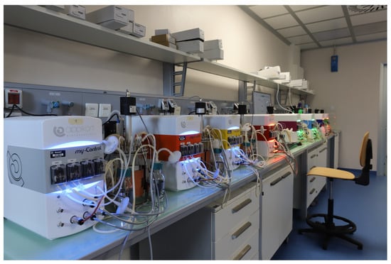
Figure 1.
Photo of the eight independent 1 L MiniBio units. Each unit was equipped with a controller dosing the different critical process parameters. All controllers were connected to a computer equipped with the Lucullus software acting as an interface and recording the process parameters.

Table 1.
Fermentations with corresponding final OD600nm, biomass, inclusion body weight, and OD600nm/IB ratio values.
2.1.3. Inclusion Body Recovery
At the end of the fermentation, biomass was harvested by centrifugation (15 min at 8000 rpm with rotor GS3 Sorvall), and the pellet was resuspended in 0.1 M Tris with 0.01 M EDTA at pH 8.0 and homogenized at 800 ± 50 bars for four 4 cycles (Panda, GEA Italia, Via Angelo Maria da Erba Edoari 29/A—43123 Parma, Italy ). The solution was then centrifuged and washed twice with the same buffer. The last pellet, corresponding to inclusion bodies, was stored at −70 °C for further use.
2.2. Machine Learning Pipeline
2.2.1. Data Preparation
This section describes the phases of data selection and pre-processing needed to prepare the data with the aim to exploit a machine learning approach.
Parameter Selection. The first step of the data preparation is the analysis of the CPPs to identify and select a subset of CPPs useful for the algorithm. Table 2 shows the selected CPP with their nomenclature in the data.
Table 2.
Critical process parameters (CPPs).
Fermentation Selection. Before performing the pre-processing, we selected a subset from the available fermentation batches (see Figure 2 and Figure 3 and also supplementary file for discarded fermenatation batches). The selection was performed considering both the quality and quantity of the data, as well as by analyzing whether the fermentation had a standard and canonical progress. Moreover, we trimmed selected data to remove missing or inconsistent values. Thus, the selected fermentations were 8, 11, 12, 16, 22, 23, 24, 25, 26, 27, and 28.
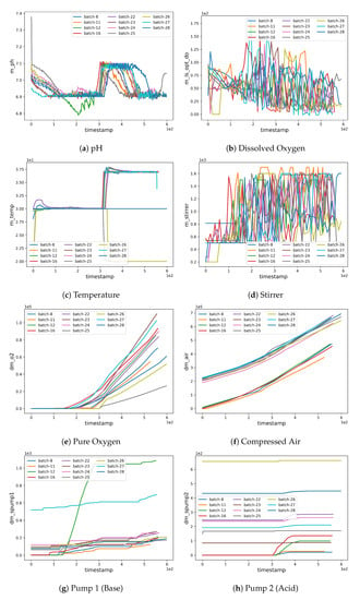
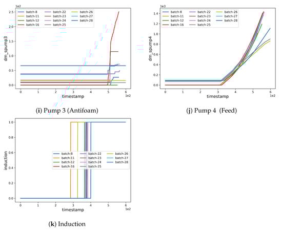
Figure 2.
Plots for the critical process parameters (CPP).
Figure 3.
Fermentation batch selection.
Cumulative to Non-Cumulative Data. Some CPPs, e.g., “spumps”, are acquired in the form of cumulative data, meaning that the sensor registers the sum between the measured value and the previously registered value at each timestamp. More formally, the current value is obtained as , where v is the registered value and m is the measured value. As a consequence, the obtained values monotonically increase during the acquisition. Nonetheless, such an implicit information codification makes it harder for the machine learning algorithm to learn hidden correlation in the data. As a consequence, because cumulative data provide the same fundamental information of non-cumulative data, the first step of data pre-processing is to transform cumulative data into non-cumulative data by defining m as follows: .
Data Normalization. Machine learning approaches require that both training and test data are equally distributed. Accordingly, we normalize the data with the standard technique of the z-score. The z-score transforms the data distribution with a mean and standard deviation into a normal Gaussian distribution with mean 0 and standard deviation 1, as follows:
where is the value after the normalization and is the standard deviation. To equally normalize both the training and test data, we select data from fermentation 16 to compute the mean and the standard deviation.
Data Sequencing. To correctly format the data being processed by the selected algorithm, we needed to create discrete data sequences through the grouping of contiguous timestamps (see Section 2.2.2). With this aim, we use an approach based on a sliding window that progressively scans and groups data together. We use a stride, meaning that the window goes through the data by jumping of a number of timestamps defined by the stride value each iteration. We set the size of the sliding window to 20 and the stride to 5.
OD600nmInterpolation. The CPP data and the OD600nm data have a temporal inconsistency, because CPP values are acquired with a frequency of one per minute, whereas the OD600nm values are acquired with a frequency of one per hour. However, the machine learning algorithm requires that the sampling frequency is equal for both the CPP and OD600nm values. To overcome this issue, we interpolate OD600nm values by linearly mixing values obtained from separately fitted linear and polynomial interpolations. Specifically, the interpolated values are obtained with the following expression:
where is the final interpolated value, is the linearly interpolated value, and is the polynomially interpolated value. We used a sixth-degree polynomial, which adds a smoothing component to the non-derivable curve obtained from local linear interpolation (piecewise linear). In doing so, we separately fit linear and polynomial interpolation curves and then linearly combined the two using and weights. By setting , we assigned the same weight to the linear and polynomial interpolation curves in the construction of the final fitted value, i.e., the arithmetic mean between the linear and polynomial interpolated values. The choice of using a sixth-degree polynomial and the choice of letting were driven by experimental observations. In fact, although these choices do not grant an overall smoothness to the final interpolating curve as would be the case by letting , the combined choice effectively reduces the intangible effect of having discontinuities in the derivative function of the final interpolating curve upon known experimental values, while at the same time preventing unrealistic swings between consecutive ones as would be the case using a fitting polynomial of a higher degree. By setting , we obtained a mean R2 score of 99.93, and an example of it is shown in Figure 4.
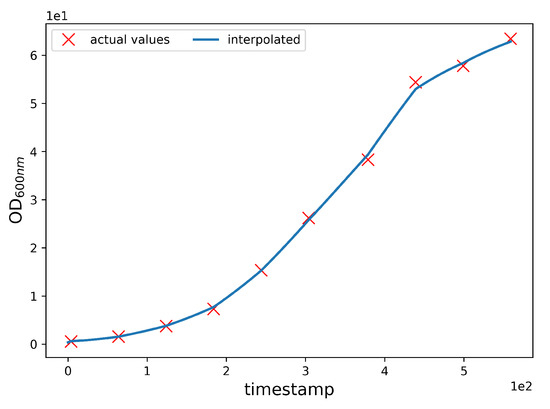
Figure 4.
Interpolation of the OD600nm values. The blue line is the interpolated data, and the red Xs are the experimental values of batch 8. The interpolation allows an effective approximation of the trend of the OD600nm values during the fermentation.
2.2.2. Deep Learning Model
Fermentation processes involve living organisms that evolve over time and, consequently, both the CPP and OD600nm values evolve as well and are strongly influenced by values assumed at previous timestamps. This evolution is handled well by machine learning models that are able to process sequences of data rather than single data, revealing hidden correlations across timestamps.
Recurrent neural networks and long-short term memory models [19] are neural networks specifically devised to work on sequential data typical of tasks such as action recognition in videos [20], language translation [21], speech recognition [22], and image captioning [23].
Different from feed-forward neural networks (FFNNs) [24], these types of models do not assume the independence of input data across time. As a consequence, when working with data sequences, the output at the current timestamp is obtained by examination of input data throughout the whole sequence, including data from past timestamps within the sliding window limits. Therefore, the input data have a size of (, s) and the output has a size of (, 1), where is the window size, and s is the number of input features. In this work, we use an architecture composed of the following modules:
- Fully connected layer;
- RNN/LSTM module;
- Fully connected layer.
The first fully connected layer allows the mapping of input data onto a high-dimensional latent space. We experimentally proved the effectiveness of this choice. Instead, the second fully connected layer allows obtaining the final OD600nm predictions. The model is illustrated in Figure 5.
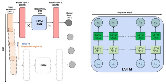
Figure 5.
Neural network architecture used for the estimation of the OD600nm (RNN cells are also considered as an option for LSTM cells). The architecture is applied to time sequences of size 20 and progressively processes the full data sequence with a stride of 5 data points. At a fixed time, 11 CPPs are given; this results in a 20 × 11 dimension of the inputs. Such inputs are individually fed to a single fully connected neural network layer and produce a new vector (hidden layer 1) which is in turn fed to a two-layer LSTM (or RNN) module. Such a module is recurrent, meaning that vectors are not processed independently in time, rather, cell outputs are fed to the cell itself at the next time instance (left figure), meaning that predictions are based on a history of 20 samples. Two extra (non-recurrent) fully connected layers are stacked to produce a one-dimensional output at each time instance, namely, the OD600nm prediction. For more details, please refer to the python code provided along with this article at https://github.com/MattiaLitrico/Smart-Fermenter (accessed on 23 May 2023).
We used a grid search method for hyperparameter value optimization, as detailed in Table 3.
Table 3.
Hyperparameters used for the network architecture.
3. Experiments
We performed experiments using the architecture described in the previous section. Both the training and testing were preceded by a data pre-processing stage. We trained our model using a learning rate of 0.001, a batch size of 256, and an SGD optimizer.
3.1. Setup
As mentioned in Section 2.2.1 (Fermentation Selection), we performed a preprocessing stage to select a subset of fermentations suitable to train, validate, and test the machine learning model. The selection criteria are based on the quality and consistency of the acquired data. Firstly, we defined the “canonical” fermentation settings, in which we removed the fermentations that have not been accomplished using the canonical settings. This category includes the preliminary fermentations used to establish the canonical settings, as well as some fermentations that use glycerol as a carbon source (see Figure 3). Secondly, we excluded fermentations that suffered from some failure during the process, as well as fermentations with no production of the recombinant protein. Lastly, we trimmed data points (mainly from the tail ends) from some of the batches (e.g., 25, 26, 28) for which we did not have periodic OD600nm readings.
3.2. Evaluation Criteria
The use of a machine learning algorithm requires the availability of both a training set and a test set. The former is the subset of the data used to train the algorithm. On the contrary, the latter is used to evaluate its prediction performances. We used the leave-one-out cross-validation (LOOCV) [25] method to evaluate the model, in which the number of folds is equal to the number of fermentations in the data set. With all other fermentations acting as a training set and the chosen fermentation acting as a single-item test set, the learning algorithm is applied once for each fermentation. By doing so (i) we were able to evaluate the generalization ability of the algorithm in various scenarios and (ii) we achieved a reliable and unbiased estimate of the model performance.
3.3. Evaluation Metrics
To evaluate the proposed approaches, we compute two metrics: root mean squared error (RMSE) [26] and relative error on final yield (REFY). The RMSE is a standard machine learning metric commonly used as a performance indicator for a regression model. By computing the square root of the mean value of the squared differences between model predictions and the ground-truth values, it gives an estimate of the model’s predictive power (accuracy). The RMSE is described by the following expression:
where is the total number of observations in the fermentation, is the model prediction, and is the ground truth OD600nm value at timestamp t.
Additionally, we introduce the REFY metric that measures the absolute error at the last timestamp of the fermentation. This allows the REFY to be influenced by only the accuracy at the end of the fermentation rather than during all the fermentation. Moreover, the final prediction is the value that matters the most. The REFY is described by the following expression:
4. Results
The quantitative results reported in Table 4 demonstrate that both networks, i.e., LSTM and RNN perform well with comparable average root mean squared error (RMSE) and relative error on final yield (REFY) values, though RNN outperforms by a slight margin. However, we observed that point-wise RMSE is slightly higher in the initial yield estimation points, which is undeniably due to the lack of context (history) available at the beginning of CPP data. However, the models generalize better as we move along the successive timestamps. We also observe a plateau in the final yield estimation points of batches 8, 12, and 25.
Table 4.
Results based on LSTM and RNN networks.
Overall, the REFY of batches 8 and 25 are comparatively high, with an average RMSE. The RMSE of batch 11 yield estimation is high for both networks, with a slightly high REFY for the LSTM network only. The yield estimation of batch 12 is comparatively the least accurate of all batches. In Section 5.2, we discuss all the potential reasons behind such outcomes. Nevertheless, yield estimation for most batches, i.e., 16, 22, 23, 24, 26, 27, and 28 are quite promising, paving the way for machine learning-based black-box modeling of the fermentation process.
5. Discussion
5.1. Production
All fermentations were run in parallel in 1 L fermenters equipped with a software interface able to store critical parameters in real time. This strategy allows execution of several fermentations in parallel and enables direct, real-time evaluation of the influence of specific parameters during the cultures. Furthermore, such a volume is a good compromise between ease of use and quantity of recombinant protein produced. This aids in setting up and optimizing downstream processes and, at the same time, providing material to preclinical pharmaceutical departments. In fact, the availability of even grams of material to be purified eases downstream process development and further related upscaling. In this project, fermentations have been developed to obtain high yields with middle cell densities. In fact, as reported in Table 1, a total of 10 to a maximum of 13.5 g of inclusion bodies can be recovered from each fermentation with OD600nm values spanning from 52 to 63. This is due to the combination of different factors such as rich culture medium, which favors Escherichia coli growth and rational design space exploration.
A further point to consider is the reduced fermentation time, which at the one-liter scale hardly exceeded 10 h. The short fermentation time combined with high inclusion body yield are very promising achievements for project upscaling and industrialization.
It is also important to note that even when expression system has been modified, as in the last four fermentations where the neurotrophic factor was engineered to be expressed in a soluble form and not accumulate in inclusion bodies, the system is still able to predict the final culture OD600nm value. This accuracy rate for network prediction was possible because the same Escherichia coli strain, expression vector, and culture medium were used. Most important, this can be considered to be a worst-case test or a special challenge that was successfully completed by the ML model. We have shown that training the ML model on a specific strain growing in a specific medium allows the same model to also predict final culture OD600nm in different conditions and with different versions of the neurotrophin expressed in a soluble or insoluble form, as detailed in the next section.
5.2. ML Prediction Results
We supply qualitative results in Figure 6 for analyzing estimation quality and initiating discussion. The high REFY performances on batches 8 and 12 are due to these batches having a final yield much higher than the average final yield (see Table 4); this is an unusual condition that made it difficult for the models to infer from the training data. Nevertheless, by examining the REFY and Figure 6a, we observe that the model performs well on batch 8 until the yield estimation settles on the final value.
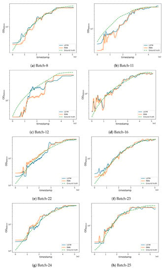
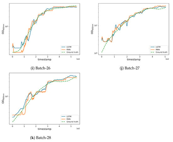
Figure 6.
Qualitative results obtained by the LSTM and RNN networks.
As can be seen in Figure 3b, batches 11 and 12 possess a different experimental yield trend (with higher values when compared to other batches) which also contributes to the higher RMSE (see Figure 6b,c where the estimations are less accurate from the very initial timestamps). Furthermore, an unusually high trend can be observed in the pump 1 () values in batches 12 and 27 which affects the corresponding yield estimates as can be noted from the magnitude of the anomaly in pump 1 (base) values (see Figure 2g). The high REFY performance on batch 25 can be explained by the very low pure oxygen () in the last timestamps of the fermentation (see Figure 2e).
Altogether, this implies that models struggle to predict the OD600nm in unusual CPP trends, i.e., trends underrepresented in the training data, with a consequent lack of generalization ability. In addition, the results highlight the importance of computing both metrics (RMSE and REFY) for capturing the real behavior of the models during all the fermentation. Nonetheless, the generalization ability could possibly be improved with more training data, further exploring the design space hyper-volume adjacent to the experimental conditions to be found in batches 8, 11, 12, and 25. Such exploration is currently out of the scope of this study, because the models’ performances and process robustness are satisfying and promising for transfer into a GMP plant for clinical production.
6. Conclusions
In this work, we demonstrated the general applicability of machine learning approaches to predict real-time and final yields of fermentation processes designed to recover recombinant proteins of biotechnological interest. We trained our ML model to predict real time OD600nm values from CPP historical series. This black-box model allows for the early termination of a process that is recognized to be diverging from normal conditions by monitoring real-time CPP values. Furthermore, it is trained on CPPs only, i.e., we did not include any MPPs as inputs, upon which (by definition) no control would be possible. Thus, the (black-box) relationship we developed between OD600nm and CPP values paves the way for a ML-driven control system by offering a reliable alternative to numerous trial-and-error experiments for identification of the optimal fermentation conditions and related yields. In fact, optimal CPP set points maximizing OD600nm value are recommended in real time by the prediction algorithm on the basis of the learned (not yet analytical) relationship inferred from the training data. The model was trained on a set of fermentations run in a short period of time and tested on very different protocols as in the last four fermentations reported in Table 1, where the fed batch phase temperature was set to 20 °C and the cultures were run overnight. Furthermore, even though culture medium and Escherichia coli strain were the same in all fermentations, the protein was expressed in a soluble form and did not accumulate in inclusion bodies. Being able to predict the final fermentation OD600nm in those conditions is a further “validation” of the ML model. In fermentation 28, the final OD600nm was lower than usual, and this can be explained by the phenomenon of cell lysis during the overnight culture phase. This cell lysis is probably due to a complete substrate depletion during the overnight induction. Exploring the design space allowed construction of a black-box relationship between the critical process parameters and the OD600nm value on the one hand, and allowed setting the best possible fermentation protocol on the other. RNN and LSTM neural networks were optimized to predict real time and final OD600nm values from fermentation CPP time series. The errors associated with yield predictions from both networks demonstrate that RNN and LSTM are promising tools to design control strategies relying upon black-box models trained on CPP time series and related yields from past fermentations.
Furthermore, it is very interesting to note that when a fermentation problem is encountered (as in run 12) the prediction cannot be accurate, because CPP trends are very different from those observed in training. This is particularly evident for run 12 in Figure 2, where we can cross compare the green pH curve (panel a) with Pump 1 (panel g) and observe that they have different trends with respect to other fermentations.
The same phenomenon can be seen in run 11, where the maximum allowed stirrer speed was set 100 rpm higher than the usual value. This higher mixing speed has a positive influence on the culture broth oxygenation. As a result, we have a lower pure oxygen consumption and as a consequence, two CCP have been concomitantly affected in this run, resulting in predictions that were only partially aligned with the ground truth towards the end of the fermentation.
In both cases, the model has been able to rapidly highlight fermentation trends that were drifting from the “normal” or expected ones. This is very encouraging for further model development with the aim of becoming the reference “expert” that is able to warn the operator driving a real GMP fermentation that a deviation from normal process is ongoing.
Supplementary Materials
The following supporting information can be downloaded at: https://www.mdpi.com/article/10.3390/fermentation9060503/s1: List and discussion of discarded fermentation batches.
Author Contributions
Conceptualization, D.B., P.M. and F.M.; data curation, D.B., M.L., T.C., E.S. and F.M.; funding acquisition, D.B. and F.M.; investigation, D.B., P.M. and F.M.; methodology, D.B., M.L. and P.M.; project administration, D.B. and F.M.; resources, W.A.; software, M.L., W.A. and P.M.; supervision, F.C., M.A., A.R.B. and A.D.B.; validation, D.B., M.L., W.A. and P.M.; visualization, M.L. and W.A.; writing—original draft, D.B., M.L., W.A., P.M. and F.M.; writing—review and editing, A.D.B. All authors have read and agreed to the published version of the manuscript.
Funding
This research was funded by the Italian Ministry Proj. no. F/190142/01/X44—CUP: B11B20000180005 Ministero Sviluppo Economico Fondo per la Crescita Sostenibile—PON I&C 2014-2020, DM 5 marzo 2018.
Institutional Review Board Statement
Not applicable.
Informed Consent Statement
Not applicable.
Data Availability Statement
The data presented in this study and the code needed to reproduce the results are openly available at https://github.com/MattiaLitrico/Smart-Fermenter (accessed on 23 May 2023).
Conflicts of Interest
The authors declare no conflict of interest. The funders had no role in the design of the study; in the collection, analyses, or interpretation of data; in the writing of the manuscript; or in the decision to publish the results.
Abbreviations
The following abbreviations are used in this manuscript:
| CPP | Critical Process Parameters |
| DO | Dissolved Oxygen |
| GMP | Good Manufacturing Practices |
| LSTM | Long Short-Term Memory Network |
| ML | Machine Learning |
| OD600nm | Optical Density (at 600 nanometers) |
| REFY | Relative Error on Final Yield |
| RMSE | Root Mean Squared Error |
| RNN | Recurrent Neural Network |
| rpm | Rotation Per Minute |
| SGD | Stochastic Gradient Descent |
| UPLC | Ultra Performance Liquid Chromatography |
References
- Rosano, G.L.; Ceccarelli, E.A. Recombinant protein expression in Escherichia coli: Advances and challenges. Front. Microbiol. 2014, 5, 172. [Google Scholar] [CrossRef] [PubMed]
- Cai, J.; Hua, F.; Yuan, L.; Tang, W.; Lu, J.; Yu, S.; Wang, X.; Hu, Y. Potential Therapeutic Effects of Neurotrophins for Acute and Chronic Neurological Diseases. BioMed Res. Int. 2014, 2014, 601084. [Google Scholar] [CrossRef]
- Huang, E.J.; Reichardt, L.F. Neurotrophins: Roles in 26 neuronal development and function. Annu. Rev. Neurosci. 2001, 24, 677–736. [Google Scholar] [CrossRef] [PubMed]
- Rattenholl, A.; Lilie, H.; Grossmann, A.; Stern, A.; Schwarz, E.; Rudolph, R. The pro-sequence facilitates folding of human nerve growth factor from Escherichia coli inclusion bodies. Eur. J. Biochem. 2001, 268, 3296–3303. [Google Scholar] [CrossRef]
- Masoudi, R.; Ioannou, M.S.; Coughlin, M.D.; Pagadala, P.; Neet, K.E.; Clewes, O.; Allen, S.J.; Dawbarn, D.; Fahnestock, M. Biological activity of nerve growth factor precursor is dependent upon relative levels of its receptors. J. Biol. Chem. 2009, 284, 18424–18433. [Google Scholar] [CrossRef] [PubMed]
- Schimek, C.; Egger, E.; Tauer, C.; Striedner, G.; Brocard, C.; Cserjan-Puschmann, M.; Hahn, R. Extraction of recombinant periplasmic proteins under industrially relevant process conditions: Selectivity and yield strongly depend on protein titer and methodology. Biotechnol. Prog. 2020, 36, e2999. [Google Scholar] [CrossRef]
- Vanti, C.V.M.; Leite, L.C.; Batista, E.A. Monitoring and control of the processes involved in the capture and filtering of biogas using FPGA embedded fuzzy logic. IEEE Lat. Am. Trans. 2015, 13, 2232–2238. [Google Scholar] [CrossRef]
- Hansen, B.D.; Tamouk, J.; Tidmarsh, C.A.; Johansen, R.; Moeslund, T.B.; Jensen, D.G. Prediction of the Methane Production in Biogas Plants Using a Combined Gompertz and Machine Learning Model. Comput. Sci. Its Appl.—ICCSA 2020, 2020, 734–745. [Google Scholar]
- Manu, D.S.; Thalla, A.K. Artificial intelligence models for predicting the performance of biological wastewater treatment plant in the removal of Kjeldahl Nitrogen from wastewater. Appl. Water Sci. 2017, 7, 3783–3791. [Google Scholar] [CrossRef]
- Nourani, V.; Elkiran, G.; Abba, S.I. Wastewater treatment plant performance analysis using artificial intelligence—An ensemble approach. Water Sci. Technol. 2018, 78, 2064–2076. [Google Scholar] [CrossRef]
- Wang, L.; Long, F.; Liao, W.; Liu, H. Prediction of anaerobic digestion performance and identification of critical operational parameters using machine learning algorithms. Bioresour. Technol. 2020, 298, 122495. [Google Scholar] [CrossRef] [PubMed]
- Cinar, S.Ö.; Cinar, S.; Kuchta, K. Machine Learning Algorithms for Temperature Management in the Anaerobic Digestion Process. Fermentation 2022, 8, 65. [Google Scholar] [CrossRef]
- Helleckes, L.M.; Hemmerich, J.; Wiechert, W.; von Lieres, E.; Grünberger, A. Machine learning in bioprocess development: From promise to practice. Trends Biotechnol. 2022, 41, 817–835. [Google Scholar] [CrossRef]
- Khaleghi, M.K.; Savizi, I.S.P.; Lewis, N.E.; Shojaosadati, S.A. Synergisms of machine learning and constraint-based modeling of metabolism for analysis and optimization of fermentation parameters. Biotechnol. J. 2021, 16, 2100212. [Google Scholar] [CrossRef]
- Chen, F.; Li, H.; Xu, Z.; Hou, S.; Yang, D. User-friendly optimization approach of fed-batch fermentation conditions for the production of iturin A using artificial neural networks and support vector machine. Electron. J. Biotechnol. 2015, 18, 273–280. [Google Scholar] [CrossRef]
- Packiam, K.A.R.; Ooi, C.W.; Li, F.; Mei, S.; Tey, B.T.; Ong, H.F.; Song, J.; Ramanan, R.N. PERISCOPE-Opt: Machine learning-based prediction of optimal fermentation conditions and yields of recombinant periplasmic protein expressed in Escherichia coli. Comput. Struct. Biotechnol. J. 2022, 20, 2909–2920. [Google Scholar] [CrossRef]
- Nagata, Y.; Chu, K.H. Optimization of a fermentation medium using neural networks and genetic algorithms. Biotechnol. Lett. 2003, 25, 1837–1842. [Google Scholar] [CrossRef] [PubMed]
- Vinitha, N.; Vasudevan, J.; Gopinath, K.P. Bioethanol production optimization through machine learning algorithm approach: Biomass characteristics, saccharification, and fermentation conditions for enzymatic hydrolysis. Biomass Conv. Bioref. 2022. [Google Scholar] [CrossRef]
- Sherstinsky, A. Fundamentals of Recurrent Neural Network (RNN) and Long Short-Term Memory (LSTM) Network. Phys. D Nonlinear Phenom. 2020, 404, 132306. [Google Scholar] [CrossRef]
- Cavazza, J.; Ahmed, W.; Volpi, R.; Morerio, P.; Bossi, F.; Willemse, C.; Wykowska, A.; Murino, V. Understanding action concepts from videos and brain activity through subjects’ consensus. Sci. Rep. 2022, 12, 19073. [Google Scholar] [CrossRef]
- Rivera-Acosta, M.; Ruiz-Varela, J.M.; Ortega-Cisneros, S.; Rivera, J.; Parra-Michel, R.; Mejia-Alvarez, P. Spelling correction real-time american sign language alphabet translation system based on yolo network and LSTM. Electronics 2021, 10, 1035. [Google Scholar] [CrossRef]
- Wang, D.; Wang, X.; Lv, S. An overview of end-to-end automatic speech recognition. Symmetry 2019, 11, 1018. [Google Scholar] [CrossRef]
- Cui, W.; He, X.; Yao, M.; Wang, Z.; Li, J.; Hao, Y.; Wu, W.; Zhao, H.; Chen, X.; Cui, W. Landslide image captioning method based on semantic gate and bi-temporal LSTM. ISPRS Int. J. -Geo-Inf. 2020, 9, 194. [Google Scholar] [CrossRef]
- Bebis, G.; Georgiopoulos, M. Feed-forward neural networks. IEEE Potentials 1994, 13, 27–31. [Google Scholar] [CrossRef]
- Sammut, C.; Webb, G.I. Leave-one-out cross-validation. Encycl. Mach. Learn. 2010, 600–601. [Google Scholar] [CrossRef]
- Hyndman, R.J.; Koehler, A.B. Another look at measures of forecast accuracy. Int. J. Forecast. 2006, 22, 679–688. [Google Scholar] [CrossRef]


Disclaimer/Publisher’s Note: The statements, opinions and data contained in all publications are solely those of the individual author(s) and contributor(s) and not of MDPI and/or the editor(s). MDPI and/or the editor(s) disclaim responsibility for any injury to people or property resulting from any ideas, methods, instructions or products referred to in the content. |
© 2023 by the authors. Licensee MDPI, Basel, Switzerland. This article is an open access article distributed under the terms and conditions of the Creative Commons Attribution (CC BY) license (https://creativecommons.org/licenses/by/4.0/).