Wineinformatics: Regression on the Grade and Price of Wines through Their Sensory Attributes

Abstract

Wineinformatics is a field that uses machine-learning and data-mining techniques to glean useful information from wine. In this work, attributes extracted from a large dataset of over 100,000 wine reviews are used to make predictions on two variables: quality based on a “100-point scale”, and price per 750 mL bottle. These predictions were built using support vector regression. Several evaluation metrics were used for model evaluation. In addition, these regression models were compared to classification accuracies achieved in a prior work. When regression was used for classification, the results were somewhat poor; however, this was expected since the main purpose of the regression was not to classify the wines. Therefore, this paper also compares the advantages and disadvantages of both classification and regression. Regression models can successfully predict within a few points of the correct grade of a wine. On average, the model was only 1.6 points away from the actual grade and off by about $13 per bottle of wine. To the best of our knowledge, this is the first work to use a large-scale dataset of wine reviews to perform regression predictions on grade and price.

1. Introduction

Wine is one of the most popular drinks in the world, with over twenty-eight billion liters produced across 63 countries in the year 2015 alone [1]. To be this popular, wine must have several interesting characteristics which humans enjoy: aroma, color, and flavor. Many computer-based techniques have been applied or developed for use in the wine field, such as software for wine-making [2] and classification of the wines’ characteristics [3]. Wineinformatics studies how these characteristics can be used to make inferences about the wine, such as the wine’s quality and how expensive it may be. Traditionally, chemical analyses have been used to represent the wines’ features [4,5,6]. Unfortunately, humans cannot intuitively appreciate a wine based on knowledge of the chemical structure as humans do not experience wines through this type of knowledge. Instead, humans understand what they perceive through sensation. Comparing a chemical description of a wine to a qualitative description of a wine based on its review, as shown in Figure 1, demonstrates how a sensory description may be more easily understood than a chemical one.

Accordingly, the chemical details do not capture the experience one has when drinking wine. The sensory description reveals flavors that may be compared to other sensations the reader (or wine consumer) may be familiar with. Although a review contains qualitative information, and is thereby subjective, there are known and trusted experts in the field of wine who make wine reviews. Many works have used wine reviews to analyze wines, and there has also been an effort to allow non-experts to contribute to building a qualitative description of wine [7,8,9,10]. Wine reviews may be generated by experts according to different policies, depending on the source. Wine Spectator generates 15,000 wine reviews each year through a specific tasting guide [11]. In order to avoid biases, all of their tastings are blind-tasted. Additionally, reviewers tend to focus on specific types of wines, so that they may become better experts on them. Some tastings may be made by multiple reviewers to ensure consistency and accuracy.

Based on these reviews, a representation of a wine can be constructed. However, in order to construct a representation of wines from these reviews, a systematic process needs to be in place. The Computational Wine Wheel 2.0 (CWW2) was selected for use in this process [12,13]. The Wine Wheel contains keywords of reviews that are important in describing the wine, such as “blackberry”. Unimportant words, such as “articles”, are discarded. These keywords were built up to a total of 985 categories of normalized wine attributes by analyzing several years of Top 100 wine reviews from Wine Spectator [12]. The Computational Wine Wheel 2.0 was then applied to a large scale dataset of over 100,000 wine reviews. Since the Computational Wine Wheel can process a large amount of wine reviews automatically, various data science techniques may be applied to discover the information that could benefit society, including wine producers, distributors, and consumers. This information may be used to answer the following questions: “Why do wines achieve a 90+ rating? What are the shared similarities among groups of wine and what wines are suggested to the consumer? What are the differences in character between wines from Bordeaux, France, and Napa, United States? What is the weather impact on the wine in the same region and grape type?” Using these extracted keywords that describe the wine in human language, this research aim was to predict the wines’ quality and price. Both of these variables can be expressed with a numerical value; therefore, regression is a perfect tool for this research.

One major factor of the wine is the grapes itself, which are affected by the terroir and weather, while another major factor is the wine-making process, which is governed by the wine-makers. Experienced wine-makers can taste the grape harvests and build up the optimal wine-making process, which contains the following five stages: harvesting, crushing and pressing, fermentation, clarification, and aging and bottling. During the “crushing and pressing” process, the flavor, color, and tannins of the wine are defined; during the “fermentation” process, the acidity, alcohol percentage, and sweetness of the wine are carefully monitored; and during the “aging and bottling” process, the final touches of the wine are overseen, such as aging in French oak barrels for a subtle, spicy, and silky texture, while aging in American oak barrels will yield a stronger flavor, such as in cream soda, vanilla, and coconut.

All of this knowledge is embedded in a wine-maker’s mind and experiences. This paper provides an opportunity to discover, from a wine reviewer’s point of view, what makes a good combination of flavor, wine body, and non-flavor descriptions (such as “pure”, “harmony”, “beauty” and “wonderful”), of the wine in terms of wine grade. This paper also offers an opportunity to reveal, from a wine-maker’s point of view and according to the taste of the wine, what may be a suitable price listed for consumers. If a perfect regression model is able to be built, wine-makers can utilize it by placing expected attributes of the wine they make to see the expected score and price. Wine-makers can also substitute some wine attributes to simulate alternative choice of wine-making (such as a French barrel vs. American barrel vs. steel tanks) to evaluate the expected wine grade and price. Therefore, the goal of this work was to use the extracted keywords to build regression models that accurately predict many wines’ quality and price. This is the first work that we are aware of in which a large-scale dataset of keyword representations of wine reviews is used to make numerical predictions on grade and price via regression.

2. Materials and Methods

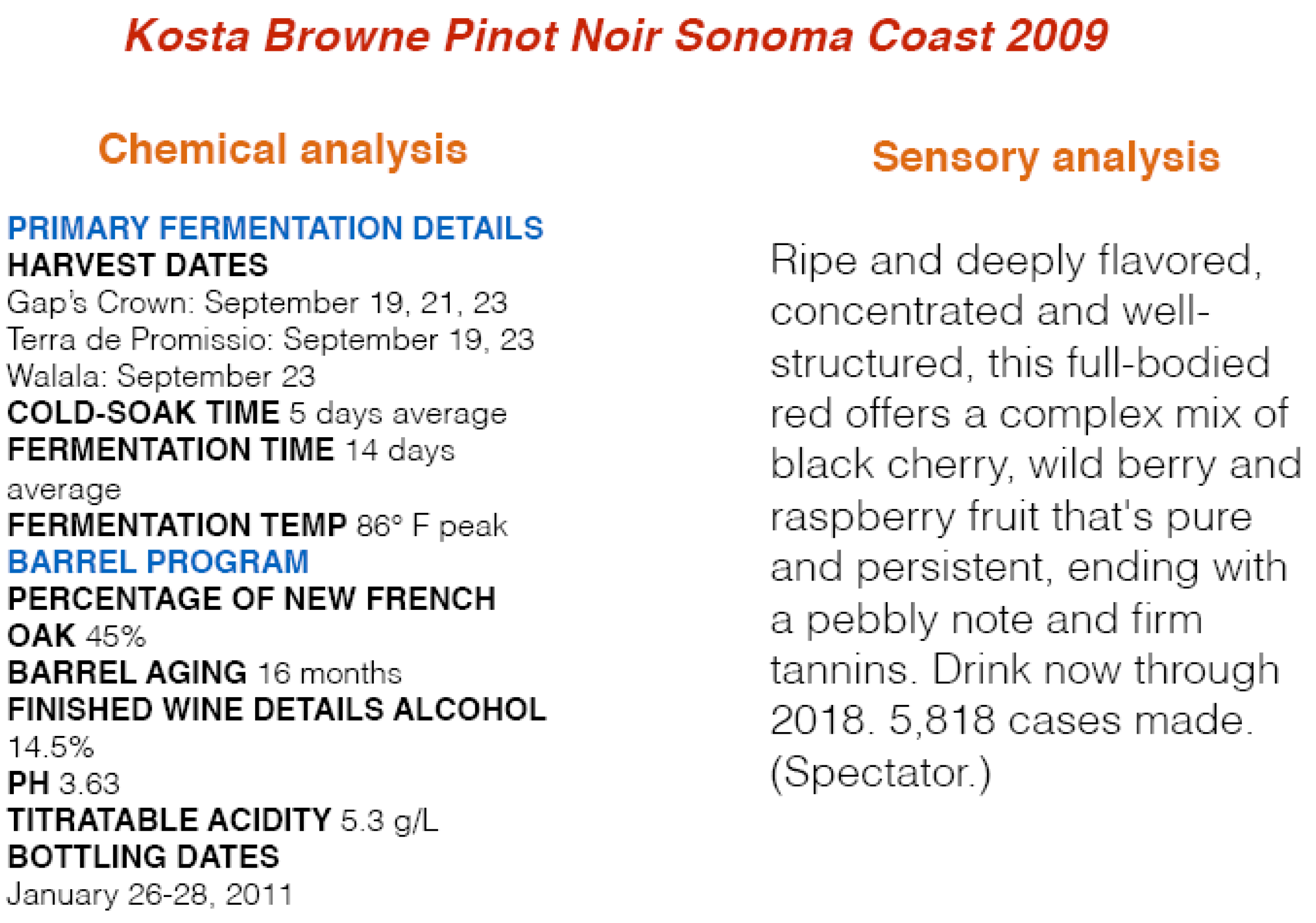
2.1. The Data

The source of the wine reviews used for this work was a website called Wine Spectator. Wines of “good” or better quality and and their reviews were pulled from the website and preprocessed. Data with missing or indecipherable information was simply omitted. 105,085 wines and their reviews ranging over a period from 2006 to 2015 remained.

The quality of the wine was judged based on Wine Spectator‘s 100-point scale. Quality ranging from 80–84 was considered good, 85–89 was very good, 90–94 was outstanding, and 95–100 was classic [14]. Prices ranged from $0 to almost $1000 per 750mL bottle of wine (a small number of wines in the dataset were listed as free). Out of the entire dataset, the Computational Wine Wheel identified 799 important key phrases (some keywords, such as “black cherry”, may have actually contained multiple words). Each phrase was considered an attribute. For each phrase, an instance was assigned either a “1” if that phrase appeared in its review, or a “0” otherwise. The phrases that occured in at least 2000 different reviews are shown in Figure 2.

The boxplots of the grades and prices are shown. Considering the distribution of the prices, there are many extreme values. This will pose a problem when considering metrics sensitive to outliers, which will be discussed in the next section. To deal with this, a second dataset was constructed where all wines with prices higher than $98, the upper whisker in the price boxplot, were removed. There are exactly 6800 wines with prices higher than $98. By removing wines with these prices, the boxplot became less dominated by extreme values, as shown in Figure 3c. This allowed us to evaluate the regression model without the influence of overly expensive wines. It should be noted, however, that the median price of classic quality wines is $112, which is higher than $98. Therefore, this price model will have less than half of the highest-quality wines incorporated.

In our prior work, classification on grade and price was utilized. These classes had to be formed by transforming the numerical values into distinct categories. For grade, Wine Spectator’s 100-point scale, described above, was used as the basis for forming the grade classes. For price, the quartiles were used to form the categories. Two different models of classification were used: a four-way multiclass classification (formed by the 100-point scale and quartiles on grade and price, respectively) and binary classification (formed by combining the lower two and upper two classes into two groups in each variable). The class breakdowns are shown in

Table 1. Response variables and their class categories for the four-class dataset and the two-class dataset.

	Category	Grade	Price
Four-class dataset	1	≤84	≤$18
	2	85~89	$19~$29
	3	90~94	$29~$50
	4	95~100	>50
Two-class dataset	1	<90	≤$29
	1	≥90	>$29

[15]. For simplicity, the different datasets will be referred to as the four-class and two-class datasets for multiclass and binary classification, respectively, and the numerical dataset for regression.

2.2. Evaluation Metrics

There are several metrics that can be used to evaluate a regression model. Most of these metrics are based on the concept of error. A regression model predicts an actual number that it thinks an instance has based on its attributes. The difference between the prediction and the actual value is called the error. If the error is positive, the model predicted a value higher than the actual value. Similarly, if the error is negative, the model predicted a value lower than the actual value. The average of all of these errors is known as the mean error (ME). This value expresses the average magnitude the model was off over all the instances.

Unfortunately, a ME of zero does not mean that the model is perfect. In fact, because positive and negative numbers cancel out when averaging them, the ME can mask significant problems with the model. A better metric is to consider the mean absolute error (MAE). This metric sacrifices the knowledge of how high or low the model tends to predict in exchange for information about how much error accumulated, on average, from the entire instance predictions. Computing this metric is the same as with ME, except one simply takes the absolute value of the error before adding it into the average.

Another metric is the mean squared error (MSE). Like the MAE, MSE considers how much error accumulated overall. Unlike MAE, MSE works by squaring the values instead of taking the absolute value. This has the disadvantage of being sensitive to outliers, which will be discussed in the section below. However, MSE is better than MAE in detecting when a few, large errors are made (while MAE is better for the exact opposite problem). Since simply squaring the errors results in enormous values, it is common to take the square root after the average is done, resulting in a root mean squared error (RMSE). This also transforms the error back into the same units as the value being predicted.

The MAE and RMSE give us measures for absolute error: that is, they give us a real number which reflects the actual value of error. This value is not normalized or compared to the range of possible values that may be taken on. Because the errors are in an absolute sense, it is not clear whether any given error is good or bad. To understand this, consider a regression model which performs with an MAE of 0.1 units. This may sound like a small error, but because there is no comparison to the actual value ranges in the data, it is impossible to determine if the error is good or bad. If the possible numeric values range from 1 to 100, then the error is quite good. On the other hand, if the possible numeric values range from 0 to 0.3, then an error of 0.1 is so large that predictions from this model are probably useless. Normalizing the MAE and RMSE allows us to better understand how good or bad the model performs.

There are two ways to normalize the error. The first way is to take the error and divide it by the range of possible values. This can be expressed by the formula:

$$\mathrm{Minimax}\mathrm{Norm}{\mathrm{Error}}_{\mathrm{y}}=\frac{Erro{r}_{\mathrm{y}}}{\max \left(\mathrm{y}\right)-\min \left(\mathrm{y}\right)}\times 100$$

(1)

where y is the variable being predicted. Multiplying by 100 transforms the relative error into an easy-to-interpret percentage value. Normalizing this way makes sense when clear boundaries can be established for the maximum and minimum values. This is also the case for grade—the minimum and maximum grades in the dataset were 80 and 100, respectively. For price, however, this method is not as suitable. While the experiment can clearly define a lower price of $0, there is no limit to how high the price of a wine may cost. Of course, the experiment could use the highest price found in the dataset. However, this may be deceiving for two reasons. First, the price dataset contains outliers. Second, because of the presence of outliers, it is likely that a new dataset could contain wines with a price higher than the wines found in the dataset used here. Third, because wines may take on a wide range of prices, with only a relatively few numbers of wines being expensive, it is more appropriate to consider how the model performs on the majority of the wines—the wines that do not cost near the maximum or minimum price. A more reliable normalization technique, one that is both robust to outliers and can describe the bulk of the data, not just the extremes, is needed. Thus, standard deviation is used for such a metric. Rather than taking the error and dividing it by the range of the data, dividing the error by the standard deviation makes the normalized error more robust to outliers and removes the need for us to know what the range of prices could be. This formula is:

$$\mathrm{St}.\mathrm{Dev}.\mathrm{Norm}{\mathrm{Error}}_{\mathrm{y}}=\frac{Erro{r}_{\mathrm{y}}}{{\mathsf{\sigma }}_{\mathrm{y}}}\times 100$$

(2)

where y is the variable being predicted and $\mathsf{\sigma }$_y is the standard deviation of the variable.

From these considerations, the minimax normalized error will be used for grade and the standard deviation normalized error will be used for price. This normalization will be applied to MAE and RMSE to form NMAE and NRMSE. Note that it does not make sense to normalize MSE in this way due to the difference in units (although one could use variance to normalize MSE, the experiment in this research will refrain from doing so).

Another metric is the coefficient of correlation (r), which measures how strongly the attributes and response variable are related, as well as providing the type of relationship. Values may be between −1 and 1, where a zero means there is no relationship. A value of 1 suggests a perfectly positive relationship and a value of −1 suggests a perfectly negative relationship. By squaring the coefficient of correlation, the coefficient of determination $r^2$ is retrieved. The coefficient of determination measures how much variance between the predicted and actual values is explained by the model, where 0 means none of the variance was explained by the model and a value of 1 means all of the variance was explained by the model. r and $r^2$, together with ME, MAE, MSE, RMSE, NMAE, and NRMSE, are used to evaluate the results generated from regression model (Section 3.1).

Compared with the research work where classification was performed, here, accuracy is used as the evaluation metric. Accuracy is defined as the percentage of the number of instances which are correctly categorized into the correct class. A perfect score is 100% accuracy. The accuracy is used evaluate the results while we convert the regression result for predicting the wine class listed in Table 1. For example, if $30 is the price of a wine generated by the regression model, by mapping the results to the class labels (Figure 1), the model predicts the wine to be a category 3 in the four-class category and a category 2 in the bi-class category. The true label can be used to compare with the predicted label for calculation of the accuracy evaluation metric.

2.3. Methods

The choice of algorithm used for performing regression was based on the Support Vector Machine (SVM); more specifically, Support Vector Regression (SVR) [16,17,18]. Support vector machines are inherently binary classifiers; they draw a hyperplane between two classes of data, such that the margin, or distance between the classes, is maximized. While acceptable for a classification problem, this method is inappropriate for a regression problem. However, the notion of drawing a hyperplane does not need to be restricted to the separation of data: one could draw a hyperplane that follows a trend in the data. That is precisely the purpose of SVR; it draws a hyperplane such that as much data as possible can fit into the margins that surround the hyperplane.

SVR contains two key hyperparameters: the kernel, and a way to control the slack in the margins, denoted as ϵ. Allowing for the slack in the margins allows for dealing with the case when not all data fits within the margins around the hyperplane. This value was left at the default of 1. The kernel allows for the SVR to transform the data into a higher dimensional space such that it is easier to construct a hyperplane which follows the data. The linear, Gaussian Radial Basis Function (RBF), and Laplacian RBF kernels are tested in this research.

The implementation of SVR was from the Kernlab package in R, with Microsoft’s R Open being the implementation of R used [19,20,21]. In order to compute the evaluation metrics, the gof function from the R package hydroGOF was used [22].

In our prior work, SVMs from two implementations (Kernlab and LibSVM via the Waikato Environment for Knowledge Analysis (WEKA)) were used to perform the classifications [23,24]. Several kernels were trialled, with the linear and RBF kernels performing the best. The cost of the constraint violation hyperparameter C, which is similar to ϵ except it is used when performing classifications, was set to 1. In all cases, both in this work and the prior work, five-fold cross validation was used to train and test the models.

3. Results

3.1. Regression

Firstly, considering only the results for running SVR on grade, shown in

Table 2. Table of results for the regression model on Grade. Normalized error is calculated using the minimax method.

Kernel	ME	MAE	MSE	RMSE	NMAE	NRMSE	r	r2
Linear	−0.07	1.64	4.27	2.07	8.2%	10.4%	0.73	0.54
RBF/Laplace	0.00	4.59	4.02	2.00	8.0%	10.0%	0.75	0.56

, all three models reported similar levels of error, with the two RBF models tying for first place. RBF and Laplace RBF demonstrated exactly the same results; therefore, we present their results as RBF/Laplace in Table 2. The zero value for ME suggested that the RBF/Laplace models were able to find a perfect balance for where to draw the hyperplane. The low value for RMSE suggested there were not many large errors; rather, there were many smaller errors, as expected with a good regression model. The normalized errors were also smaller, suggesting that the model can predict within about 8% (1.6 points) of the actual value of the instance. The coefficients of correlation and determination were also good values, suggesting a strong positive relationship and suggesting the model can explain the majority of the variance between the independent and dependent variables.

Next, consider the results for running SVR on price, as shown in

Table 3. Table of results for the regression model on price. The normalized error is calculated using the standard deviation method.

Kernel	ME	MAE	MSE	RMSE	NMAE	NRMSE	r	r2
Linear	−9.56	20.53	2082.15	45.63	41.8%	93.0%	0.44	0.19
RBF/Laplace	−9.88	20.52	2133.56	46.19	41.8%	94.2%	0.43	0.18

. There was a clear evidence of outliers; the MSE values were very large, and the RMSE was over twice the value of MAE, suggesting that there were at least several large errors. In addition, the ME was very negative, suggesting that the actual values were higher than the model’s predictions. This would be the case for large positive outliers. Note that the normalized errors were not comparable to the normalized errors for grade, since the method of calculation is different (indeed, if the method used here were minimax, the normalized errors would be around 2–4% ($19–$38)). This interpretation for NMAE was that the predicted price was almost half a standard deviation away from the actual value. Similarly, the NRMSE said that the predicted price (when squaring and rooting the error) was almost a whole standard deviation away from the actual value. Both of these values suggested there was some room for improvement; a large number of wines can be contained within a standard deviation of the mean price point.

Of the three kernels, the linear model, being less sensitive to outliers, was reporting better results than the RBF/Laplace models. By removing the outliers, significantly better results were yielded, shown in

Table 4. Table of results for the regression model on price, without outliers. The normalized error is calculated using the standard deviation method.

Kernel	ME	MAE	MSE	RMSE	NMAE	NRMSE	r	r2
Linear	−3.80	13.07	325.25	18.03	64.3%	88.7%	0.50	0.25
RBF/Laplace	−3.75	12.94	318.64	17.85	63.6%	87.8%	0.51	0.27

, allowing the RBF and Laplacian kernels to retake the lead. As for actual performance, the ME decreased to a third of its original size. Although it was still negative, suggesting there may still be some outliers in the new dataset, the RMSE was much smaller than before. In addition, the RMSE was no longer over twice as large as the MAE, which also decreased. Unfortunately, the NMAE increased, while, interestingly, the NRMSE decreased. This can be explained by the standard deviation being cut by nearly half, from around $40 with outliers to around $20 without outliers. The NMAE was not as sensitive to the removal of outliers as NRMSE, but both were equally sensitive to the change in standard deviation, leading to one increasing while the other decreased. Making the transition from a dataset with outliers to a dataset without outliers justifies the use of standard deviation for computing normalized error; the normalized minimax errors on the dataset without outliers would be around 13–17%. The large drop in price range drove up the normalized error, even though the model performs better without outliers. Improved performance was clearly observed by considering the coefficients of correlation and determination; they both increased by a good amount, suggesting a much stronger relationship and a model which explains more of the variance than before.

3.2. Classification

In our prior work, excellent classification accuracies were achieved by LibSVM with Linear kernel; Binary Grade (90+/90−) prediction accuracy was as high as 85.92%, and Multiclass Grade (80~84/85~89/90~94/95+) prediction accuracy was 75.22%; Binary Price ($29+/$29−) prediction accuracy was 74.85%, and Multiclass Grade ($\le$$18/$19~$29/$29~$50/≥$50) prediction accuracy was 48.71%. It would be nice to compare the regression results to the classification results. It can be achieved by checking to see if the predicted value from the regression model can be converted to the same class value that the actual value would be converted to. For example, if the actual grade is 84 and the predicted grade is 82, both of these can be mapped to the “good” grade category, and so the regression model would be considered to have classified this instance correctly. Conversely, if the actual grade is 84 and the predicted grade is 85, the regression model is considered incorrect, even though the error is smaller, because a grade 85 wine is a “very good” wine. This means that errors along borderline wines are going to cost the regression model more than errors along non-borderline wines. The regression models provide more information than the classification models, so the use case for a regression model is different than for classification. For these reasons, lower classification accuracy from the regression model does not at all imply that the model is any worse. In fact, it is actually better for the regression model to perform worse at the classification task in exchange for better metrics found in the tables above.

The multi-class classification accuracy for grade using the RBF kernel was 66.53%, while the multi-class classification accuracy for price using the linear kernel was 38.1%. When the outliers are removed, the linear model performs worse, with an accuracy of 34.0%. However, this may be explained by the reduced number of outliers: the 6000 fewer outliers was about 5.7% of the data, a little over the percentage of accuracy lost. Since the outliers were not close to the boundaries between the classes, the loss of these instances means that misclassifications along border instances are a more frequent occurrence. This would outweigh any of the gains made in predicting the other instances by removing the outliers. In other words, the removal of the outliers should be expected to reduce classification accuracy, since outliers are easier to classify than instances along class boundaries.

4. Discussion

Through our study, it was shown that regression models can successfully predict within a few points of the correct grade of a wine. On average, our model was only 1.6 points away from the actual grade given by Wine Spectator if the errors do not cancel each other out. Regression models can also predict price, although it is more difficult to predict; on average, our model was off by about $13 per bottle of wine. These were not exactly stellar results: a hypothetical consumer could easily be swayed by a price difference of $13 in all but the most expensive wines. This got even worse when outliers were present; the predictions were off by an accumulated average of $20.53. Fortunately, the mean error was negative at −$4 without outliers, suggesting that the model would be more likely to tell a hypothetical consumer that the price was more expensive than it really is, not less. This may be desirable if sticker shock is to be avoided; however it may also persuade customers not to consider the wine at all. Nevertheless, regression provides considerably more granular information than that provided by classification. Even though regression cannot be used to make good classifications, a misclassification (via either model) could result in an error many more points or dollars away than the errors achieved by regression.

This work shows that useful regression models on grade and price can be constructed from the review attributes on a large-scale dataset. It is important that such a construction can be made; wine reviews are made from human experiences with wine, and these experiences may be positive or negative. Positive experiences would be reflected in a high-quality rating. Since it is non-trivial to produce high-quality wine and since humans prefer positive experiences, the price of wine will be influenced by these reviews as well. Unfortunately, economic forces outside the scope of the review will likely contribute to greater difficulty in building a regression model for it. Nevertheless, a useful model can still be built. Wine reviews are a qualitative and subjective expression of the wine. In sum, this paper showed, for the first time, that key phrases from reviews may be used to accurately predict both the grade and price of wines.

References

1. Wine Institute. World Wine Production by Country. Available online: https://www.wineinstitute.org/files/WorldWineProductionbyCountry.pdf (accessed on 28 September 2018).
2. Schmidt, D.; Freund, M.; Velten, K. End-User Software for Efficient Sensor Placement in Jacketed Wine Tanks. Fermentation 2018, 4, 42. [Google Scholar] [CrossRef]
3. Sommer, S.; Cohen, S.D. Comparison of Different Extraction Methods to Predict Anthocyanin Concentration and Color Characteristics of Red Wines. Fermentation 2018, 4, 39. [Google Scholar] [CrossRef]
4. Er, Y.; Atasoy, A. The classification of white wine and red wine according to their physicochemical qualities. Int. J. Intell. Syst. Appl. Eng. 2016, 4, 23–26. [Google Scholar] [CrossRef]
5. Cortez, P.; Cerdeira, A.; Almeida, F.; Matos, T.; Reis, J. Modeling wine preferences by data mining from physicochemical properties. Decis. Support Syst. 2009, 47, 547–553. [Google Scholar] [CrossRef] [Green Version]
6. Ebeler, S.E. Linking flavor chemistry to sensory analysis of wine. In Flavor Chemistry; Springer: Boston, MA, USA, 1999; pp. 409–421. [Google Scholar]
7. Chen, B.; Velchev, V.; Nicholson, B.; Garrison, J.; Iwamura, M.; Battisto, R. (2015, December). Wineinformatics: Uncork Napa’s Cabernet Sauvignon by Association Rule Based Classification. In Proceedings of the 2015 IEEE 14th International Conference on Machine Learning and Applications (ICMLA), Miami, FL, USA, 9–11 December 2015; pp. 565–569. [Google Scholar]
8. Chen, B.; Le, H.; Rhodes, C.; Che, D. Understanding the Wine Judges and Evaluating the Consistency through White-Box Classification Algorithms. In Industrial Conference on Data Mining; Springer: Cham, Germany, 2016; pp. 239–252. [Google Scholar]
9. Wariishi, N.; Flanagan, B.; Suzuki, T.; Hirokawa, S. Sentiment Analysis of Wine Aroma. In Proceedings of the 2015 IIAI 4th International Congress on Advanced Applied Informatics (IIAI-AAI), Okayama, Japan, 12–16 July 2015; pp. 207–212. [Google Scholar]
10. Flanagan, B.; Wariishi, N.; Suzuki, T.; Hirokawa, S. Predicting and visualizing wine characteristics through analysis of tasting notes from viewpoints. In International Conference on Human-Computer Interaction; Springer: Cham, Germany, 2015; pp. 613–619. [Google Scholar]
11. About Our Tastings. Available online: https://www.winespectator.com/display/show/id/scoring-scale (accessed on 28 September 2018).
12. Chen, B.; Rhodes, C.; Yu, A.; Velchev, V. The Computational Wine Wheel 2.0 and the TriMax Triclustering in Wineinformatics. In Industrial Conference on Data Mining; Springer: Cham, Germany, 2016; pp. 223–238. [Google Scholar]
13. Chen, B.; Rhodes, C.; Crawford, A.; Hambuchen, L. Wineinformatics: Applying data mining on wine sensory reviews processed by the computational wine wheel. In Proceedings of the 2014 IEEE International Conference on Data Mining Workshop (ICDMW), Shenzhen, China, 14 December 2014; pp. 142–149. [Google Scholar]
14. Wine Spectator’s 100-Point Scale. Available online: http://www.winespectator.com/display/show/id/scoring-scale (accessed on 28 September 2018).
15. Palmer, J. Multi-Target Classification and Regression in Wineinformatics. Ph.D. Thesis, University of Central Arkansas, Conway, AR, USA, 2018. [Google Scholar]
16. Fradkin, D.; Muchnik, I. Support vector machines for classification. DIMACS Ser. Discret. Math. Theor. Comput. Sci. 2006, 70, 13–20. [Google Scholar]
17. Martin, L. A Simple Introduction to Support Vector Machines; Michigan State University: East Lansing, MI, USA, 2011. [Google Scholar]
18. Smits, G.F.; Jordaan, E.M. Improved SVM regression using mixtures of kernels. In Proceedings of the 2002 International Joint Conference on Neural Networks, Honolulu, HI, USA, 12–17 May 2002; Volume 3, pp. 2785–2790. [Google Scholar]
19. R Core Team. R: A Language and Environment for Statistical Computing, R Foundation for Statistical Computing, Vienna, Austria. Available online: https://www.R-project.org (accessed on 28 September 2018).
20. Microsoft and R. C. Team, Microsoft R Open, Microsoft, Redmond, Washington, 2017. Available online: https://mran.microsoft.com/ (accessed on 28 September 2018).
21. Karatzoglou, A.; Smola, A.; Hornik, K.; Zeileis, A. Kernlab-an S4 package for kernel methods in R. J. Stat. Softw. 2004, 11, 1–20. [Google Scholar] [CrossRef]
22. Mauricio Zambrano-Bigiarini, hydroGOF: Goodness-of-Fit Functions for Comparison of Simulated and Observed Hydrological Time Series, 2017, r Package Version 0.3-10. Available online: http://hzambran.github.io/hydroGOF/ (accessed on 28 September 2018).
23. Chang, C.C.; Lin, C.J. LIBSVM: A library for support vector machines. ACM Trans. Intell. Syst. Technol. (TIST) 2011, 2, 27. [Google Scholar] [CrossRef]
24. Hall, M.; Frank, E.; Holmes, G.; Pfahringer, B.; Reutemann, P.; Witten, I.H. The WEKA data mining software: An update. ACM SIGKDD Explor. Newsl. 2009, 11, 10–18. [Google Scholar] [CrossRef]
Figure 1. Review of the Kosta Browne Pinot Noir Sonoma Coast 2009 (scores 95 pts) on both chemical and sensory analysis.
Fermentation 04 00084 g001
Figure 2. A word cloud of all of the keywords that occured in at least 2000 different wine reviews. The size of the word corresponds to its frequency.
Fermentation 04 00084 g002
Figure 3. Boxplots of price with outliers (a), price without outliers (b), and grade (c).
Fermentation 04 00084 g003