Agronomical and Chemical Effects of the Timing of Cluster Thinning on Pinot Noir (Clone 115) Grapes and Wines

Abstract

A two-year study was performed to evaluate the effects of the timing of cluster thinning on Pinot noir grapes and wines in the central coast of California. Vines were thinned to one cluster per shoot at three selected time-points during the growing season, and fruit was harvested and made into wine. No consistent effect of cluster thinning was found in wine phenolic profile or color across a cool (2016) and a warm (2017) growing season. The growing season had a more significant effect than the cluster thinning treatment for most parameters measured. There was no detectable overall sensory difference between the non-thinned control wines and any of the thinned treatment wines. Based on current results, Pinot noir vineyards on the central coast of California can support crop loads that result in Ravaz Index values from 3 to 6 without concern for impacting ripening potential or negatively affecting fruit composition.

1. Introduction

Pinot noir (Vitis vinifera L.) is a challenging grape cultivar from both a viticultural and winemaking perspective. Viticulturally, Pinot noir grapevines produce compact clusters of thin-skinned berries, which increase susceptibility to fungal pathogens relative to other V. vinifera cultivars. Pinot noir grapes (and their wines) are also inherently low in phenols [1,2]. Phenols are biomolecules originally present in the grapes (and subsequently extracted into wine). Phenols can be broadly classified as simple phenols having a C6–C1 or C6–C3 structure and a single aromatic ring containing one or more hydroxyl groups; and polyphenols, which contain multiple phenol rings and are defined by a C6–C3–C6 structure bearing hydroxyl and non-hydroxyl substitutions [3]. In wines, polyphenols are responsible for color [4,5,6], tactile sensations such as astringency [7,8], and taste sensations such as bitterness [9,10,11]. In addition to sensory effects on astringency, taste, and aroma modulation [12], flavonoids also play a critical role in the chemical stability of the wine during aging as these molecules intervene in metal-catalyzed oxidation reactions [13,14]. Because of the relatively lower phenolic content of Pinot noir, wines produced from it are lighter in color and astringency than wines made from other cultivars [15]. Pinot noir is also notable for lacking acylated anthocyanins [2], which are abundant in other cultivars such as Cabernet Sauvignon or Syrah and may in turn provide more stable color [16,17]. As color is one of the main drivers of perceived wine quality [18], viticultural practices such as cluster thinning are often applied to Pinot noir grapes in an attempt to lower yields and influence fruit polyphenol composition by lowering vine crop load [19,20,21,22,23,24,25].

Polyphenols such as anthocyanins and tannins, and their reaction products, known as polymeric pigments [8], are positively associated with wine quality [18]. In turn, and as mentioned above, vineyard crop load manipulation techniques such as cluster thinning are often applied to influence phenolic development [19,20,21,22,23,24,25]. The traditional yield to fruit quality paradigm of a linear relationship with quality increasing as yield decreases [24,25,26,27], has been shown to be an oversimplification, and yields are more accurately described as a function of vine balance [28,29]. Vine balance, better described as the source/sink ratio, relates vine vegetative and reproductive growth, either through leaf area/yield (LA/Y) ratios [30] or through the ratio between dormant vine pruning weights and yields, the latter known as the Ravaz Index [31,32]. For most cultivars, in warm climates, 0.8–1.2 m² of leaf area is needed to ripen 1 kg of fruit, which generally results in a yield/pruning weight ratio of 5 to 10 [30].

Crop load metrics are dependent upon vine capacity, which is in turn influenced by regional and viticultural factors such as climate [33], canopy training and trellising [34], rootstock, and cultivar [21,35]. Grapes grown in cool climates require higher source/sink ratios than those grown in warmer regions because of lower daytime temperatures that restrict both leaf photosynthetic capacity and berry carbon assimilation [29,34,36]. As a result of this restricted photosynthetic capacity, the ability of grapes grown in cool climates to ripen fruit to commercially viable total soluble solids (TSS) levels is limited and is significantly affected by seasonal variations in weather [33,34]. As such, in cool climates, seasonal variations in weather may have a greater effect than the source/sink ratio on Pinot noir ripening [33].

Despite the prevalence of cluster thinning in Pinot noir, few studies have been conducted to investigate the effects of this viticultural technique on this cultivar. Indeed, most studies on cluster thinning have been conducted in warm, arid climates and on cultivars such as Cabernet Sauvignon [37,38] and Tempranillo [22,24,39]. The bulk of this research suggests conflicting results, whereby it has not been conclusively shown that manipulating yields by cluster thinning will uniformly affect fruit composition. For example, some research has indicated that cluster thinning can positively impact fruit composition [26,27,40], while other studies have found no effect on fruit composition [21,38,41,42] or that the effect of cluster thinning was dependent upon the climate conditions of any single growing season [20,21,24]. In other instances, compositional effects as a result of cluster thinning have been found in grapes, but these have not translated into the finished wines [27]. Pinot noir grown in cool climates may be more suited to benefit from cluster thinning because of the inherently low polyphenol content of the fruit and reduced carbon assimilation capacity of vines in cool climates [29,34,36].

The timing of cluster thinning may also have an impact on vine physiology and fruit composition. For example, it has been hypothesized that removing crop at bloom may lead to lower leaf transpiration rates, and therefore lower leaf photosynthesis rates [43], which could negate the desired effect of enhanced berry ripeness [21]. In addition, if photosynthesis rates remain unchanged but the source/sink ratio increases upon cluster thinning, the increased photo-assimilates may stimulate vegetative growth, counteracting or negating the benefits of the decreased crop load [29,32]. In a study spanning five seasons, early thinning at bloom increased berry weight in Cabernet Sauvignon, Riesling, and Chenin blanc, while late thinning performed at véraison was intermediate to early thinning and non-thinned vines [21]. However, this effect was not found in all years of the previous study. Cluster thinning applied at bloom to Pinot noir vines resulted in increased berry size [19], although there was no late thinning treatment included in the study. Other research has shown no effect of thinning on berry size in Tempranillo [22], thereby suggesting that there is likely a cultivar-specific response of berry size as a result of cluster thinning. Berry size reduction has traditionally been considered desirable from a winemaking perspective based on the empirical assumption that comparatively smaller berries have higher berry surface area/volume than larger ones. However, the relationship between berry size and phenolic composition is not a simple linear relationship, as berry skin and seed mass grow along with berry size [44], and therefore larger berries may not be necessarily undesirable as once thought. Multiple studies conducted with a variety of cultivars investigating the relationship between cluster thinning and berry size have found conflicting results dependent upon cultivar and growing season [19,21,22], and as such, there is no current conclusive understanding of the relationship between cluster thinning and berry size, and the subsequent effect of the latter on wine composition.

In the central coast of California (USA), consisting of Santa Barbara, San Luis Obispo, and Monterey counties, there are over 7000 hectares of Pinot noir being grown [45], representing a substantial contribution to the wine industry of the region. Indeed, in 2016, wine grapes were the most valuable crop produced in San Luis Obispo County [46]. Despite the economic importance of Pinot noir on the central coast of California, no research has been undertaken to understand the relationship between Pinot noir crop load and fruit quality in the cool climate of San Luis Obispo county of the central coast. While research in cooler areas such as Oregon’s Willamette Valley (USA) have indicated that grape ripeness increased in a curvilinear fashion with increasing LA/Y ratios up to 1.25–1.75 m²/kg [34], which is higher than the LA/Y ratios observed in warm climates [30], these source/sink ratios are intrinsically tied to the seasonal limitations of the region that result in inconsistent ripening and may not be translatable to more moderate cool climates such as California’s central coast.

In the present study, the effect of crop load reduction by cluster thinning was explored for the first time on Pinot noir grapes (clone 115) and wines grown in the cool climate conditions of the Edna Valley of the Central Coast (San Luis Obispo County) of California (USA). The objectives of this study were to evaluate the effect of the timing of cluster thinning crop reduction on vine capacity, berry composition, and wine composition over two consecutive seasons. An additional objective was to identify appropriate crop loads in cool climate Pinot noir grown on the central coast of California.

2. Materials and Methods

2.1. Vineyard Site

This study was conducted at a commercial vineyard located in Edna Valley (35°11′58.3″ N 120°34′12.6″ W), San Luis Obispo County, California, during the 2016 and 2017 growing seasons. Treatments of cluster thinning were applied to Pinot noir grapevines (clone 115) planted in 1996 on 5C rootstock. Cluster thinning was applied to these Pinot noir grapevines at selected phenological growth stages. Cluster thinning was conducted by removing the second cluster from each fruiting shoot of the vine. Any third clusters (second crop) were also removed during the treatment, resulting in one cluster per fruiting shoot. No second crop thinning or reduction was performed in the control vines. Vineyard treatments were applied as 100-vine sets replicated five times (n = 5), organized as a randomized complete block. Bloom was defined as stage 23 on the modified Eichhorn and Lorenz scale [47], and occurred on 1 June in 2016 and 15 May in 2017. Cluster thinning was applied at four weeks post-bloom (bloom + 4) approximating fruit set, eight weeks post-bloom (bloom + 8) approximating véraison, and 12 weeks post bloom (bloom + 12) shortly before harvest. Vines were pruned to two ten bud canes trained in a vertical shoot positioning (VSP) system with two catch-wires. Canes removed during the 2018 winter pruning were collected and weighed on a per-vine basis to determine 2017 growing season vegetative growth. Vine spacing was 2.75 × 1.52 m in north–south aligned rows planted in silty clay loam soil. Precipitation and daily minimum and maximum temperatures were recorded from California Irrigation Information Management System (CIMIS) weather station 52 (35°18′19.6″ N 120°39′42.4″ W), located 14.41 km from the experimental site. Cumulative growing degree days (GDD) were calculated using a baseline temperature of 10 °C and the average daily temperature from 1 April to 31 October of each year [48].

2.2. Winemaking

Fruit was harvested when a composite sample of all treatments (n = 25, 250 berries each) reached 22.5 Brix. Harvest dates were 6 September 2016 and 6 September 2017. Fruit was harvested manually from three independent vineyard replications of each treatment (n = 3). Approximately 80 kg of fruit per replicate was harvested both in 2016 and 2017, for a total of 960 kg of fruit harvested in each season. The three replicates of each of the five treatments were independently destemmed and crushed using a crusher–destemmer (Bucher Vaslin, Niederweningen, Switzerland), and placed separately in individual 60-L plastic containers (Speidel, Swabia, Germany), where fermentation took place. Musts were inoculated with a commercial wine yeast (Saccharomyces cerevisiae, EC-1118, Lallemand, Rexdale, ON, Canada) at a rate of 30 g/hL. Musts were inoculated with commercial malolactic bacteria 48 h after crushing to ensure a standardized fermentation across treatments. In 2016, musts were inoculated with VP-41 (Oenococcus oeni, Scott Laboratories, CA, USA); in 2017, musts were inoculated with ML Prime (Lactobacillus plantarum, Lallemand, Rexdale, ON, Canada). Temperature and Brix were followed daily during alcoholic fermentation using a density meter (Anton Paar, Graz, Austria) with temperature and sugar consumption curves showing good reproducibility within replicates of the same and different treatments (data not shown). Following 10 days of maceration, wines were drained off from solids, with free run wines immediately transferred to 20-L glass carboys fitted with airlocks until the completion of malolactic fermentation. Following the completion of malolactic fermentation, wines were adjusted to 0.3 mg/L molecular SO₂, bottled using a DIAM 5 microagglomerated cork closure (G3 Enterprises, Modesto, CA, USA) and kept in cellar-like conditions until analysis.

2.3. Fruit Composition

Berry chemistry and physical properties were measured at harvest from random samples of 250 berries taken from each replication (n = 3). Brix was measured using a density meter (Anton Paar, Graz, Austria); titratable acidity (TA) was measured by titrating a known quantity of juice (5 mL) in a deionized water solution against 0.067 N NaOH (Fisher Scientific, Waltham, MA, USA) to a pH endpoint of 8.2 in accordance with an established procedure (Iland et al., 2004); pH was measured with a Benchtop pH meter (ThermoFisher Scientific, Waltham, MA, USA. Yeast assimilable nitrogen (YAN) was measured enzymatically from juice utilizing an analyzer and commercially available kits (Biosystems, Barcelona, Spain). Individual vine pruning weights were taken during vine dormancy and compared with individual vine fruit yields to calculate vine Ravaz Index [31,32].

2.4. Wine Composition

Wine titratable acidity (TA) and pH were measured in the same method as juice TA and pH. Wine ethanol was measured with an alcolyzer wine M/ME analysis system (Anton Paar, Graz, Austria); wine residual sugars, acetic acid, lactic acid, and malic acid were measured with a Y15 analyzer (Biosystems, Barcelona, Spain) using commercial enzymatic analysis kits (Biosystems, Barcelona, Spain). Wine phenolics and color were measured at pressing and following the completion of malolactic fermentation (malic acid < 0.4 g/L). Anthocyanins, non-tannin phenolics, small polymeric pigments (SPP), large polymeric pigments (LPP), and total polymeric pigments (herein reported as SPP + LPP), were measured as previously described [49]. Tannins in the wines were analyzed by protein precipitation [50]. Full-visible-spectrum absorbance scans were taken using a spectrophotometer (Cary UV-VIS60, Agilent Technologies, Santa Clara, CA, USA) and absorbance data is used to construct visible light absorbance curves and run through Cary WINUV Color module software (Agilent Technologies, Santa Clara, CA, USA) to extract CIE-L*a*b* tri-stimulus colorimetry values (D65 illuminant).

2.5. Duo-Trio Test

The 2016 wines were analyzed three months after bottling for overall sensory difference using a duo-trio test with constant reference as described [51]. Briefly, the test was administered to 21 enology students of the Wine and Viticulture Department, Cal Poly San Luis Obispo. After a brief training session (1 h) to familiarize the subjects with the test, each subject received three consecutive flights, each containing three wine ISO glasses (Libbey, Toledo, OH, USA). One glass was labeled as R (“reference”) and the other two glasses were labeled with three-digit random code numbers. All the treatment replicates were contrasted against all the replicates of the control treatment. Significance was established at p < 0.05 and for n = 21, 15 correct responses were needed to establish an overall sensory difference between any of the control wines and any of the cluster thinning treatments [51]. The wines were poured 30 min before the sessions and glasses were covered with plastic lids to trap volatiles, with each glass receiving exactly 25 mL of wine.

2.6. Statistical Analyses

Statistical analyses were carried out with JMP (SAS Institute, Cary, NC, USA) for analyses of variance (ANOVA). Fisher’s least significant difference (LSD) test at the α = 0.05 level was used for means separation. Two-way ANOVA models considering treatment and growing season were carried out for all parameters with data from both growing seasons.

3. Results

3.1. Seasonal Climate

Weather data from the San Luis Obispo CIMIS weather station (Station 52, located 14.41 km from the vineyard site) was used to calculate climatological parameters during the study (

Table 1. Growing degree days (GDD); Winkler region classification; and precipitation for San Luis Obispo, California (USA).

Year	Growing Degree Days (GDD) 1	Winkler Region	Annual Precipitation (mm) 2	Seasonal Precipitation (mm) 3
2016	1462.1	II	521.9	66.2
2017	1780.6	III	733.6	79.7

¹ Calculated from 1 April–31 October in Celsius units with a baseline of 10 °C; ² Sum of precipitation from 1 January–31 December; ³ Sum of precipitation from 1 April–31 October.

). Growing degree days (GDD) were calculated for each season of the study. While GDD accumulation in 2016 placed the vineyard site in region II, considered to be a ‘cool climate’, there was sufficient heat in 2017 during the growing season to classify San Luis Obispo as region III, which corresponds with a ‘moderately warm’ climate [48].

3.2. Yield

As intended, all cluster thinning treatments resulted in a reduction of clusters per vine and vine fruit yield relative to the unthinned control (

Table 2. Two-way analysis of variance (ANOVA) with interaction showing mean values and p-values of vine yield components by cluster thinning treatment. Combined two-year averages followed by standard error of the mean. Also shown are p-values corresponding to main effects and the interaction between treatments and growing season. Different letters within a column indicate significant differences between treatment groups for Fisher’s least significant difference (LSD) test at p < 0.05. p values below 0.05 are shown in bold fonts.

Treatment	Clusters per Vine	Yield per Vine (kg)	Cluster Weight (g)	Berry Weight (g)
Control	32.13 ± 3.05 a	2.43 ± 0.34 a	74.80 ± 6.35 a	1.08 ± 0.06 a
Bloom + 4	21.06 ± 3.03 b	1.27 ± 0.14 b	64.42 ± 5.98 ab	1.05 ± 0.03 a
Bloom + 8	21.52 ± 0.99 b	1.34 ± 0.15 b	58.82 ± 5.78 b	0.96 ± 0.03 a
Bloom + 12	22.10 ± 1.59 b	1.44 ± 0.15 b	65.91 ± 6.35 ab	1.07 ± 0.07 a
Treatment (T)	0.0228	0.0029	0.2179	0.3189
Growing Season (S)	0.7436	0.0569	0.0008	0.0489
T × S Interaction	0.8149	0.6569	0.8883	0.5432

). There was no significant difference in either cluster number or vine yield between thinning treatments, indicating that the thinning treatment was evenly applied. Cluster weight was lower in bloom + 8 relative to control fruit (Table 2). However, the growing season had a larger effect on cluster weight than the thinning treatments, with cluster weights being significantly higher in the warmer 2017 growing season than in the cooler 2016 growing season (

Table A1. Vine fruit yield and fruit physical composition by treatment and growing season. Treatment means followed by standard error of the mean. Different letters within a column and growing season indicate significant differences between treatment groups for Fisher’s least significant difference (LSD) test at p < 0.05.

Growing Season	Treatment	Clusters per Vine	Vine Yield (kg)	Cluster Weight (g)	Berry Weight (g)	Seed Weight (g)	Seeds per Berry	Pruning Weight (kg)	Ravaz Index
2016	Control	33 ± 4.93 a	2.10 ± 0.34 a	63.18 ± 1.31 a	1.18 ± 0.01 a	ND 1	ND	ND	ND
	Bloom + 4	22.4 ± 5.29 ab	1.27 ± 0.25 b	58.86 ± 7.21 a	1.08 ± 0.04 ab	ND	ND	ND	ND
	Bloom + 8	20.1 ± 0.77 b	1.04 ± 0.16 b	51.35 ± 6.33 a	0.97 ± 0.01 b	ND	ND	ND	ND
	Bloom + 12	23.1 ± 2.74 ab	1.24 ± 0.03 b	54.70 ± 5.87 a	1.12 ± 0.10 ab	ND	ND	ND	ND
	p Values	0.1701	0.0461	0.519	0.0986	ND	ND	ND	ND
2017	Control	32.30 ± 4.64 a	2.76 ± 0.59 a	86.42 ± 8.04 a	0.98 ± 0.07 a	0.060 ± 0.007 a	1.37 ± 0.05 a	0.86 ± 0.06 a	3.23 ± 0.79 a
	Bloom + 4	19.10 ± 0.95 b	1.27 ± 0.19 b	72.77 ± 9.23 a	1.01 ± 0.06 a	0.042 ± 0.009 a	1.19 ± 0.12 a	0.73 ± 0.08 a	1.67 ± 0.17 b
	Bloom + 8	23.70 ± 0.30 ab	1.63 ± 0.05 b	70.02 ± 2.07 a	0.95 ± 0.06 a	0.052 ± 0.000 a	1.44 ± 0.06 a	0.91 ± 0.06 a	1.91 ± 0.15 ab
	Bloom + 12	21.10 ± 2.03 b	1.64 ± 0.26 b	77.12 ± 6.45 a	1.01 ± 0.11 a	0.051 ± 0.004 a	1.30 ± 0.11 a	0.83 ± 0.06 a	2.01 ± 0.34 ab
	p Values	0.1179	0.0616	0.4665	0.9446	0.2773	0.3983	0.1921	0.1352

¹ ND: Not determined.

in Appendix A). Berry weight was generally unaffected by the timing of cluster thinning, with the effect of the growing season having a significant impact on this parameter. Indeed, berry weight was generally higher in the cooler 2016 growing season (Table A1). No significant treatment × growing season interaction was found in any yield component, indicating that the effect of the timing of cluster thinning on yield components was equivalent in both the cooler 2016 and warmer 2017 growing seasons. In addition, in 2017, pruning weights were collected and the Ravaz index was calculated to assess vine balance. Non-thinned control vines had a Ravaz Index of 3.23 (Table A1). The Ravaz Index was lower in bloom + 4 vines relative to control vines; bloom + 8 and bloom + 12 vines were indistinguishable from control vines or one another (Table A1).

3.3. Fruit Composition

All treatments were harvested manually on a single day in both 2016 and 2017.

Table 3. Two-way analysis of variance (ANOVA) with interaction showing mean values and p-values of fruit composition parameters at harvest by cluster thinning treatment. Combined two-year averages followed by standard error of the mean. Also shown are p-values corresponding to main effects and the interaction between treatments and growing season (n = 3). Different letters within a column indicate significant differences between treatment groups for Fisher’s LSD at p < 0.05. p values below 0.05 are shown in bold fonts.

Treatment	Brix	pH	Titratable Acidity (g/L)
Control	22.28 ± 0.30 a	3.54 ± 0.03 a	6.35 ± 0.17 a
Bloom + 4	22.42 ± 0.24 a	3.53 ± 0.04 ab	6.37 ± 0.12 a
Bloom + 8	22.72 ± 0.14 a	3.55 ± 0.04 a	6.35 ± 0.14 a
Bloom + 12	22.22 ± 0.19 a	3.48 ± 0.05 b	6.59 ± 0.50 a
Treatment (T)	0.3237	0.0896	0.725
Growing Season (S)	0.4125	<0.0001	0.0115
T × S Interaction	0.0585	0.3955	0.001

shows Brix, titratable acidity (TA), and pH, which were determined at harvest. No significant difference was found in Brix level at harvest between treatments or between growing seasons (Table 3), indicating no effect of cluster thinning at any point during the growing season on the ability of fruit to ripen at this site. Fruit pH was lower in bloom + 12 relative to all other treatments and the non-thinned control (Table 3). There was a significant effect of the growing season on fruit pH, indicating that the growing season had a larger effect than treatments on fruit pH, with the cooler season resulting in lower fruit pH (

Table A2. Fruit chemical composition by treatment and growing season. Treatment means followed by standard error of the mean. Different letters within a column and growing season indicate significant differences between treatment groups for Fisher’s LSD at p < 0.05. p values below 0.05 are shown in bold fonts. TA—titratable acidity.

Growing Season	Treatment	Fruit Brix	Fruit pH	Fruit TA (g/L)
2016	Control	22.73 ± 0.43 a	3.48 ± 0.04 a	6.03 ± 0.17 b
	Bloom + 4	22.67 ± 0.44 a	3.44 ± 0.03 a	6.47 ± 0.19 b
	Bloom + 8	22.70 ± 0.26 a	3.47 ± 0.02 a	6.63 ± 0.15 ab
	Bloom + 12	21.87 ± 0.15 a	3.37 ± 0.05 a	7.53 ± 0.53 a
	p	0.2908	0.2142	0.0433
2017	Control	21.83 ± 0.27 b	3.60 ± 0.01 a	6.68 ± 0.13 a
	Bloom + 4	22.17 ± 0.17 ab	3.61 ± 0.01 a	6.28 ± 0.15 ab
	Bloom + 8	22.73 ± 0.15 a	3.62 ± 0.01 a	6.08 ± 0.04 bc
	Bloom + 12	22.57 ± 0.19 a	3.59 ± 0.02 a	5.65 ± 0.28 c
	p	0.0475	0.2944	0.0184

). There was no significant treatment × growing season interaction on fruit Brix or pH, suggesting that the effect of cluster thinning timing (or lack thereof) was the same across both a warm growing season (2017) and a cool growing season (2016). No consistent effect of treatment on fruit TA was seen across both growing seasons (Table 3). In 2016, which was the cooler growing season, bloom + 12 showed higher fruit TA relative to control fruit and in 2017, the warmer growing season, bloom + 12 had lower fruit TA relative to control fruit (Table A2). However, no difference was observed in 2017 (Table A2). There was a significant interaction of treatment and growing season, indicating that the effect of cluster thinning timing on fruit TA was dependent on environmental factors pertaining to the climate of the individual growing seasons.

3.4. Wine Composition

3.4.1. Wine Basic Chemistry

Basic wine chemistry was analyzed on the finished wines at the time of bottling. Bloom + 4 wine had higher pH relative to the control and bloom + 12 wines (

Table 4. Two-way analysis of variance (ANOVA) with interaction showing mean values and p-values of wine composition parameters post-malolactic fermentation by cluster thinning treatment. Combined two-year averages followed by standard error of the mean. Also shown are p-values corresponding to main effects and the interaction between treatments and growing season (n = 3). Different letters within a column indicate significant differences between treatment groups for Fisher’s LSD at p < 0.05. p values below 0.05 are shown in bold fonts.

Treatment	pH	Ethanol (% v/v)	Titratable Acidity (g/L)	Acetic Acid (g/L)	Lactic Acid (g/L)	Malic Acid (g/L)	Residual Sugar (g/L)
Control	3.81 ± 0.03 b	13.03 ± 0.16 a	5.36 ± 0.29 a	0.25 ± 0.04 b	1.23 ± 0.06 b	0.09 ± 0.03 a	0.45 ± 0.03 ab
Bloom + 4	3.86 ± 0.03 a	13.05 ± 0.16 a	4.91 ± 0.25 a	0.31 ± 0.03 a	1.32 ± 0.06 a	0.09 ± 0.02 a	0.43 ± 0.02 ab
Bloom + 8	3.84 ± 0.03 ab	13.17 ± 0.16 a	5.21 ± 0.24 a	0.31 ± 0.02 a	1.25 ± 0.07 b	0.04 ± 0.02 a	0.41 ± 0.02 b
Bloom + 12	3.77 ± 0.02 c	13.24 ± 0.12 a	5.25 ± 0.16 a	0.24 ± 0.04 b	1.32 ± 0.05 a	0.06 ± 0.03 a	0.47 ± 0.01 a
Treatment (T)	0.0002	0.4711	0.2637	<0.0001	0.0046	0.4302	0.1378
Growing Season (S)	<0.0001	0.0002	<0.0001	<0.0001	<0.0001	0.6511	0.0024
T × S Interaction	0.2238	0.7141	0.6896	0.0031	0.2296	0.5036	0.8459

). The growing season also significantly affected wine pH (Table 4), with pH being higher in the warmer growing 2017 season. However, there was not a significant treatment × growing season interaction, indicating that while seasonal variation in environment did influence wine pH, the effect of cluster thinning on wine pH was not affected by seasonal variation. No effect of thinning treatment was found on wine TA (Table 4). Wine TA levels were significantly higher in 2016 than 2017, indicating an effect of the growing season (

Table A4. Wine chemical composition post-malolactic fermentation by treatment and growing season. Treatment means followed by standard error of the mean. Different letters within a column and growing season indicate significant differences between treatment groups for Fisher’s LSD at p < 0.05. p values below 0.05 are shown in bold fonts.

Growing Season	Treatment	L-Malic (g/L)	L-Lactic (g/L)	Residual Sugar (g/L)	Acetic Acid (g/L)	EtOH (% v/v)	pH	Titratable Acidity (g/L)
2016	Control	0.08 ± 0.00 a	1.12 ± 0.03 bc	0.48 ± 0.04 a	0.34 ± 0.01 ab	13.18 ± 0.32 a	3.75 ± 0.01 a	5.67 ± 0.03 a
	Bloom + 4	0.07 ± 0.04 a	1.18 ± 0.00 ab	0.46 ± 0.02 a	0.35 ± 0.01 a	13.35 ± 0.14 a	3.79 ± 0.02 a	5.47 ± 0.07 b
	Bloom + 8	0.07 ± 0.02 a	1.11 ± 0.00 c	0.45 ± 0.03 a	0.35 ± 0.01 a	13.48 ± 0.16 a	3.77 ± 0.02 a	5.67 ± 0.03 a
	Bloom + 12	0.04 ± 0.01 a	1.23 ± 0.03 a	0.49 ± 0.02 a	0.32 ± 0.01 b	13.50 ± 0.02 a	3.73 ± 0.02 a	5.60 ± 0.06 ab
	p	0.6627	0.0111	0.8018	0.062	0.6209	0.214	0.0672
2017	Control	0.11 ± 0.06 a	1.35 ± 0.05 ab	0.42 ± 0.04 ab	0.16 ± 0.01 b	12.88 ± 0.10 a	3.86 ± 0.01 b	5.05 ± 0.56 a
	Bloom + 4	0.10 ± 0.04 a	1.46 ± 0.01 a	0.39 ± 0.01 ab	0.26 ± 0.03 a	12.74 ± 0.14 a	3.94 ± 0.01 a	4.35 ± 0.09 a
	Bloom + 8	0.01 ± 0.01 a	1.40 ± 0.02 a	0.37 ± 0.01 b	0.28 ± 0.01 a	12.87 ± 0.07 a	3.91 ± 0.01 a	4.75 ± 0.26 a
	Bloom + 12	0.08 ± 0.06 a	1.42 ± 0.03 b	0.45 ± 0.01 a	0.16 ± 0.01 b	12.98 ± 0.09 a	3.81 ± 0.02 c	4.90 ± 0.05 a
	p	0.4522	0.1326	0.1003	0.0021	0.5106	0.0006	0.4772

). No effect of thinning treatment was found on ethanol (Table 4). However, wine ethanol levels were higher in 2016 than in 2017 (Table A4), indicating, once again, a significant effect of the growing season over the cluster thinning treatments on the basic chemistry of the resulting wines. Bloom + 4 and bloom + 8 wines had significantly higher acetic acid levels relative to control and bloom + 12 wines (Table 4), which were statistically indistinguishable from one another. Bloom + 4 and bloom + 8 thinning treatments resulted in higher wine acetic acid levels relative to bloom + 12 and control wines (Table 4), which were statistically indistinguishable from one another. Wine acetic acid was lower in 2017 relative to 2016 (Table A4), and a significant interaction of treatment and growing season was observed (Table 4), indicating that seasonal variation in climate affected the impact of cluster thinning treatments on wine acetic acid. Although there were differences observed in wine acetic acid, because of the low nature of the acetic acid levels in the wines, these differences are unlikely to be of sensory relevance.

3.4.2. Wine Phenolics

Wine phenolics, including anthocyanins, tannins, polymeric pigments, and total phenolics, were measured as previously described [49]. There was no effect of cluster thinning treatment on wine anthocyanins or polymeric pigments in either growing season (

Table 5. Two-way analysis of variance (ANOVA) with interaction showing mean values and p-values of wine phenolic parameters post-malolactic fermentation by cluster thinning treatment. Combined two-year averages followed by standard error of the mean. Also shown are p-values corresponding to main effects and the interaction between treatments and growing season (n = 3). Different letters within a column indicate significant differences between treatment groups for Fisher’s LSD at p < 0.05. p values below 0.05 are shown in bold fonts.

Treatment	Anthocyanins (mg/L Malvidin Equivalents)	Polymeric Pigments (Absorbance at 520 nm)	Tannins (mg/L CE 1)	Non-Tannin Phenolics (mg/L CE 1)	Total Phenolics (mg/L CE 1)
Control	193.29 ± 2.80 a	0.86 ± 0.14 a	22.85 ± 7.43 ab	520.11 ± 20.64 ab	542.96 ± 22.86 ab
Bloom + 4	197.43 ± 4.00 a	0.95 ± 0.11 a	26.99 ± 4.35 a	553.86 ± 11.40 a	580.85 ± 8.85 a
Bloom + 8	197.56 ± 3.96 a	0.82 ± 0.10 a	16.64 ± 1.42 ab	516.66 ± 16.87 b	533.30 ± 16.29 b
Bloom + 12	197.22 ± 5.43 a	0.85 ± 0.10 a	14.66 ± 0.94 b	522.81 ± 10.91 ab	537.46 ± 10.92 b
Treatment (T)	0.8413	0.4305	0.1078	0.1629	0.1175
Growing Season (S)	0.2201	<0.0001	0.0304	0.0183	0.1208
T × S Interaction	0.2255	0.8451	0.1186	0.0672	0.2156

¹ CE: Catechin equivalents.

). Total phenolics, the summation of total tannins and non-tannin phenolics, was significantly higher in bloom + 4 relative to other cluster thinning treatments, although none of the treatments were statistically distinguishable from the control (Table 5). Polymeric pigments, tannins, and non-tannin phenolics exhibited greater differences due to seasonal variation than to the cluster thinning treatment (Table 5), with polymeric pigments and tannins being lower in the warmer season than in the cooler season and non-tannin phenolics being higher in the warmer season (

Table A6. Wine Phenolic profile post-malolactic fermentation by treatment and growing season. Treatment means followed by standard error of the mean. Different letters within a column and growing season indicate significant differences between treatment groups for Fisher’s LSD at p < 0.05. p values below 0.05 are shown in bold font.

Growing Season	Treatment	Total Anthocyanins (mg/L Malvidin Equivalents)	Total Polymeric Pigments (Absorbance at 520 nm)	Total Tannins (mg/L Catechin Equivalents)	Total Phenolics (mg/L Catechin Equivalents)	Non-Tannin Phenolics (mg/L Catechin Equivalents)
2016	Control	191.41 ± 4.09 a	1.13 ± 0.15 a	31.70 ± 14.01 a	519.61 ± 45.10 a	487.91 ± 32.40 a
	Bloom + 4	199.07 ± 8.70 a	1.16 ± 0.05 a	36.35 ± 2.36 a	574.75 ± 16.31 a	538.40 ± 17.35 a
	Bloom + 8	197.44 ± 8.52 a	1.04 ± 0.07 a	17.36 ± 2.86 a	503.71 ± 18.50 a	486.35 ± 20.19 a
	Bloom + 12	187.57 ± 7.13 a	1.07 ± 0.06 a	13.19 ± 1.34 a	549.21 ± 16.60 a	536.03 ± 15.42 a
	p	0.6755	0.7662	0.1500	0.3215	0.2481
2017	Control	195.17 ± 4.37 b	0.59 ± 0.01 a	14.00 ± 1.08 b	566.31 ± 5.92 a	552.31 ± 6.52 a
	Bloom + 4	195.78 ± 1.22 b	0.74 ± 0.13 a	17.63 ± 1.22 a	586.96 ± 9.42 a	569.32 ± 10.49 a
	Bloom + 8	197.67 ± 2.37 b	0.61 ± 0.01 a	15.92 ± 1.15 ab	562.89 ± 10.46 a	546.97 ± 9.83 a
	Bloom + 12	206.86 ± 1.85 a	0.64 ± 0.02 a	16.13 ± 0.67 ab	525.71 ± 13.49 b	509.59 ± 13.52 b
	p	0.0522	0.4078	0.1905	0.0171	0.0203

).

3.4.3. Wine Color

Wine CIE L*a*b* color space values were determined in the finished wines at bottling. Bloom + 12 wines exhibited higher a* and chroma than bloom + 4 and bloom + 8 wines, but all were statistically indistinguishable from control wines (

Table 6. Two-way analysis of variance (ANOVA) with interaction showing mean values and p-values of wine CIE L*a*b* chromatic parameters post-malolactic fermentation by cluster thinning treatment. Combined two-year averages followed by standard error of the mean. Also shown are p-values corresponding to main effects and the interaction between treatments and growing season (n = 3). Different letters within a column indicate significant differences between treatment groups for Fisher’s LSD at p < 0.05. p values below 0.05 are shown in bold fonts.

Treatment	L*	a*	b*	Hue Angle	Chroma
Control	85.34 ± 2.14 a	18.37 ± 2.60 ab	2.51 ± 1.53 a	−0.86 ± 0.60 a	19.03 ± 2.31 ab
Bloom + 4	85.67 ± 2.32 a	17.67 ± 2.79 b	2.55 ± 1.38 a	−0.34 ± 0.54 a	18.31 ± 2.51 b
Bloom + 8	85.85 ± 2.24 a	17.71 ± 2.61 b	2.65 ± 1.39 a	−0.28 ± 0.49 a	18.36 ± 2.32 b
Bloom + 12	84.37 ± 1.80 a	19.57 ± 2.46 a	2.71 ± 1.62 a	−0.77 ± 0.54 a	20.24 ± 2.17 a
Treatment (T)	0.1982	0.1149	0.8018	0.4819	0.1072
Growing Season (S)	<0.0001	<0.0001	<0.0001	<0.0001	<0.0001
T × S Interaction	0.3599	0.8472	0.067	0.5101	0.8306

). No effect of cluster thinning treatment was found in wine L*, b*, or hue angle. The growing season had a comparatively higher impact than cluster thinning treatment in every chromatic parameter (Table 6), with 2016 wines having lower L*, b*, and hue angle than 2017 wines, and higher a* and chroma than 2017 wines (

Table A5. Wine chromatic parameters post-malolactic fermentation by treatment and growing season. Treatment means followed by standard error of the mean. Different letters within a column and growing season indicate significant differences between treatment groups for Fisher’s LSD at p < 0.05. p values below 0.05 are shown in bold fonts.

Growing Season	Treatment	L*	a*	b*	Hue	Chroma
2016	Control	80.63 ± 0.75 a	24.13 ± 0.69 a	−0.90 ± 0.12 a	−2.17 ± 0.32 a	24.13 ± 0.69 a
	Bloom + 4	80.60 ± 1.01 a	23.73 ± 1.39 a	−0.50 ± 0.40 a	−1.13 ± 0.92 a	23.73 ± 1.39 a
	Bloom + 8	80.93 ± 0.86 a	23.47 ± 0.90 a	−0.43 ± 0.35 a	−1.00 ± 0.81 a	23.47 ± 0.90 a
	Bloom + 12	80.50 ± 1.03 a	24.90 ± 1.26 a	−0.90 ± 0.12 a	−1.97 ± 0.18 a	24.90 ± 1.26 a
	p	0.988	0.8069	0.5211	0.5131	0.8069
2017	Control	90.05 ± 0.24 a	12.61 ± 0.43 b	5.91 ± 0.19 ab	0.44 ± 0.02 a	13.94 ± 0.40 b
	Bloom + 4	90.74 ± 0.54 a	11.61 ± 0.36 b	5.60 ± 0.11 b	0.45 ± 0.00 a	12.89 ± 0.37 b
	Bloom + 8	90.76 ± 0.32 a	11.96 ± 0.39 b	5.72 ± 0.14 b	0.45 ± 0.01 a	13.26 ± 0.41 b
	Bloom + 12	88.24 ± 0.38 b	14.25 ± 0.45 a	6.31 ± 0.15 a	0.42 ± 0.01 a	15.59 ± 0.42 a
	p	0.0053	0.0079	0.0402	0.2863	0.0062

). No treatment × growing season interaction was found in any chromatic parameter.

3.5. Duo-Trio Test

Figure 1 shows a duo-trio test performed in the 2016 wines three months after bottling. Under the “constant reference” variant of this test, each wine treatment is contrasted against the control [51]. The results of this test indicated that none of the cluster thinning treatments produced wines that had overall sensory differences relative to the control wine. The panel (n = 22) failed to find an overall sensory difference between the control and any of the cluster thinning wines.

Based on these results, and considering that a panel of four experience industry professionals deemed the differences in the 2017 wines to be even less evident than those in 2016, no sensory analysis was performed in the 2017 wines.

4. Discussion

A study was conducted over two growing seasons (2016 and 2017) to determine the agronomical effects (on grapes) and chemical effects (on the resulting wines) of cluster thinning timing in Pinot noir grown in the Edna Valley of California’s central coast. A secondary objective of the study was to identify appropriate crop loads for Pinot noir on the moderately cool climate of California’s central coast. Cluster thinning treatments were applied at 4, 8, and 12 weeks post-bloom, approximating the timing of the phenological growth events of fruit set and véraison and including a pre-harvest “red drop”. Thinning consisted of removing any second or third cluster from fruit bearing shoots, reducing cluster number by an average of 34.3% across all treatments (Table 2), and reducing yield by an average of 44.4% across all treatments (Table 2). Previous studies conducted on cluster thinning practices have applied variable yield reduction rates depending on cultivar. However, most research in Pinot noir has applied “half crop” treatments such as the one performed in the current study, removing all but the basal cluster on each fruiting shoot [34] or reducing cluster number by 50% [19].

Growing degree day (GDD) accumulation varied between 2016 and 2017 enough to place each growing season in a separate Winkler Index region, with 2017 being warmer by 318.5 GDD than 2016 and qualifying as a region III (Table 1). An increase in average temperature by 1 °C increases GDD by 214 over the course of a growing season. The GDD variation observed at this site between 2016 and 2017 corresponds to approximately 1.5 °C higher average temperatures in 2017. It is well documented that vine capacity and the ability to achieve ripeness by Brix accumulation in cool regions is dependent upon climatic conditions such as temperature [48,52,53], with a base level of temperature required to adequately ripen fruit. However, Brix accumulation is not driven solely by temperature and, by extension, by GDD accumulation. In fact, differences in berry temperature may not directly impact Brix accumulation at all [52]. Indeed, other factors such as soil moisture content [54] and berry light exposure [55] may also impact fruit ripening rate irrespective of atmospheric temperature and may even have a larger effect than GDD accumulation in cases where GDD accumulation is adequate for fruit ripening [54]. Consequently, in the present study, there was no significant effect of the growing season on Brix at harvest to indicate an impact of the increased GDD accumulation in 2017 (Table 3), despite the fruit being picked on the same date in both growing seasons.

In the present study, there was no impact of the thinning treatments on Brix accumulation. However, the climatic conditions of the growing season did have a clear impact on fruit pH and TA (Table 3), resulting in lower TA and higher pH in 2017 fruit (Table A2). While bloom + 12 fruit did have significantly lower pH than control fruit (Table 3), after accounting for growing season in the model, the effect of cluster thinning treatment was not significant, indicating that the climatic conditions prevalent during the growing season had a greater effect on fruit pH and TA than cluster thinning timing. The decrease of malate concentration in grapes post-véraison through respiration increases with temperature and light exposure [56,57]; as such, the decrease in TA and the corresponding increase in pH observed in 2017, which was the warmer season (Table A2), is likely a function of the increased temperature. There was a significant treatment × growing season interaction found in TA (Table 3). In both growing seasons, bloom + 12 fruit had significantly different TA from the control treatment. However, the direction of the difference varied, with bloom + 12 having higher TA in 2016 and lower TA in 2017 relative to the control treatment. In both growing seasons, bloom + 4 was indistinguishable from the control treatment. Bloom + 8 was indistinguishable from the control or any treatment in 2016 and significantly lower than the control in 2017. Overall, there was no consistent effect of cluster thinning on fruit TA across both growing seasons (Table 3). Previous studies on Pinot noir, in which half of the crop was thinned, have found increased pH [19,53] in both fruit and juice, but mixed effects on TA, showing either no impact [19] or a reduction in TA with cluster thinning [53]. While no significant treatment effect of pH was found in the present study after considering the growing season, the inconsistent results observed in bloom + 12 fruit is similar to what has been found in previous research, suggesting the influence of some external factor on malate degradation in late-thinned fruit. It is possible that late thinning resulted in more convective heat exchange between clusters and air within the canopy, which, given the substantially warmer air temperatures in August of 2017 (

Table A7. Daily weather data from California Irrigation Information Management System (CIMIS) weather station 52 in San Luis Obispo during the 2016 and 2017 growing seasons. Daily average air temperature, minimum air temperature, and maximum air temperature.

Date	2016 Average Air Temperature (°C)	2016 Minimum Air Temperature (°C)	2016 Maximum Air Temperature (°C)	2017 Daily Average Air Temperature (°C)	2017 Minimum Air Temperature (°C)	2017 Maximum Air Temperature (°C)
1-Apr	14.2	7.3	21.5	15.8	6.7	25.8
2-Apr	12	5.2	21.9	14	7.7	21.4
3-Apr	11.7	8.1	18	14.3	9.1	22.3
4-Apr	16.5	8.3	25.4	15.1	9.1	22.8
5-Apr	22.9	14.2	30	16.6	9	25.2
6-Apr	21.9	13.1	33.2	15.5	9.8	21.2
7-Apr	15.5	11.4	21.7	14.9	13.1	16.1
8-Apr	14.7	13.4	16.7	13.1	9.3	16.5
9-Apr	15.9	12.7	20.9	13	8.8	20.9
10-Apr	15.2	12.5	20	15.7	10.2	23.2
11-Apr	14.9	12	20.5	14.7	9.2	22.4
12-Apr	13.8	9.6	19.4	15	10.1	20.5
13-Apr	14.7	9.2	21.1	13.7	8.4	17.5
14-Apr	13.1	6.6	19.1	13.7	8.7	21.7
15-Apr	14.9	10	20.1	16.6	10.3	25.5
16-Apr	17.3	9.2	26.1	15.2	8.6	22.5
17-Apr	18.6	7.7	30	15.3	12.6	18.7
18-Apr	17.9	7.4	29.6	14.6	12.2	17.7
19-Apr	17.6	8.7	28.5	16	10.8	21.4
20-Apr	15.5	5.9	25.6	17.1	10.4	23.9
21-Apr	14.9	7.2	22.6	18.6	12.7	27.5
22-Apr	14.3	7.7	21.2	17.1	11	26
23-Apr	14.5	7.8	20.2	15.8	11.1	22.3
24-Apr	14.3	6.6	20.2	15.1	11	20.4
25-Apr	10.5	3.4	16.8	14.8	11.5	19
26-Apr	11.8	5.1	19.9	16.2	13	23.7
27-Apr	12.7	6	19.5	16.2	11.1	22.5
28-Apr	11.5	5.2	17.7	16.4	11.7	23.9
29-Apr	12.1	8.3	18.5	18.3	10.6	26.2
30-Apr	14.1	7.3	21.3	18.1	9.5	27.7
1-May	15.3	7.8	23.1	23.6	15	31.8
2-May	14.5	11.5	20.7	23.9	16.8	31.7
3-May	14.3	10	23.1	21.5	14.6	27.1
4-May	14	11.4	19.4	16.8	12.3	26.7
5-May	15.5	12.9	19.8	14.5	10.5	23.1
6-May	14.7	9.9	20.3	11.4	8.4	15.1
7-May	14.8	9.7	20.5	11.3	9.2	15.4
8-May	14.3	7.6	20.9	13	7.8	19.1
9-May	15	12.3	20.2	14	9.4	19.8
10-May	14.6	11.9	20	14.8	13.2	17.6
11-May	15	12.3	20.2	15.7	11.4	21.1
12-May	14.6	11.7	20.3	14.6	10.4	20.8
13-May	14.1	11.6	18.8	13.4	9.1	18.8
14-May	15.3	8.5	21.4	12.4	7.4	17.2
15-May	15	10.5	20.1	12	7.9	16.6
16-May	14.2	9	20	13.1	9.6	17.9
17-May	15.7	10.7	22.4	13.1	9.5	18.2
18-May	16.3	9.9	25.3	16.9	9.3	27.1
19-May	13.5	11.5	19.7	21.5	11.7	29.2
20-May	13.3	9.2	16.9	19.6	10.9	29.4
21-May	12.9	6.2	18.1	17.9	10.5	27.9
22-May	13.3	5.9	19.4	16.2	10.3	24.6
23-May	14	6.9	19.8	16.3	11.7	24.2
24-May	14.6	11.9	19.1	15.3	11.6	23.6
25-May	14.7	11.6	18.5	15.3	13.8	18.5
26-May	14	8.4	18.8	15.5	10.8	19.9
27-May	15.1	10.5	21.5	15.2	8.2	21.5
28-May	15.4	10.6	21.8	15.9	10.6	21.5
29-May	15.3	12.6	21	15.7	12.7	20.8
30-May	15.6	12	22.4	15.7	11.9	22.4
31-May	16	10.4	24.6	17.4	11.4	24.7
1-Jun	16	11.2	23.4	17.9	12.8	26.7
2-Jun	16.2	10	27.1	19	13.1	29.2
3-Jun	19.4	9.5	29	18.6	12.4	26.3
4-Jun	18.8	11.9	32.4	17.4	10.6	25.4
5-Jun	15.9	10.3	23.1	16.8	10.7	26
6-Jun	15.9	11.9	22.3	16.7	10.7	24.7
7-Jun	15.9	12.3	22.8	16.7	12.5	23.1
8-Jun	16	11.8	22.1	17.4	9.7	24.9
9-Jun	15.2	11.4	20.4	18.1	14.5	23.4
10-Jun	16.6	11.5	24.7	16.6	10.1	23.8
11-Jun	16.3	10.7	21.8	15.5	9.6	23.5
12-Jun	17.5	11.6	22.2	16	8.8	23.3
13-Jun	15.7	11.4	21.4	17.7	12	26.5
14-Jun	15	8.7	21.8	21.1	14.7	28.8
15-Jun	13.5	7.4	18.7	23.5	14.6	30.3
16-Jun	16	8.4	23.4	24.7	18.8	31.9
17-Jun	16.8	9.9	24.8	26.7	18.3	32.3
18-Jun	18.5	12.4	27.1	23.3	17.9	29.5
19-Jun	22.3	12.6	31.9	21.8	13.5	32.5
20-Jun	23.6	14.5	33.6	18.6	13	29
21-Jun	24.3	14.3	32.9	17.9	12.7	26.1
22-Jun	17.5	10.3	27.2	19.2	11.8	29.1
23-Jun	21.6	9.7	34.3	18.9	15	26.1
24-Jun	19.4	11.6	25.9	18.3	14.1	24.7
25-Jun	21.7	12	34.3	18.3	13.2	26.4
26-Jun	23.6	13.9	34.4	19.5	10.7	30.4
27-Jun	26.7	17	35.3	18.4	13.4	28.3
28-Jun	22.4	12.5	30.7	17.8	13.1	25.6
29-Jun	16.8	11.4	24	17.4	12.7	26.7
30-Jun	14.7	10.2	21.9	17.3	12.4	27.4
1-Jul	16.5	11.6	23.1	16.8	12.3	23.5
2-Jul	17.3	12.6	23.4	18.2	13.3	25
3-Jul	16.3	11.6	23	19	12.9	26.4
4-Jul	15.7	10.2	21.7	18.6	10.8	28.2
5-Jul	16	13.1	22.7	19.5	13.9	31.5
6-Jul	15.6	12.2	22.1	22	15.3	30.3
7-Jul	15.7	12.3	21.8	26.1	16.5	35.9
8-Jul	16.1	11.7	24.1		17.6	38
9-Jul	18.2	11.9	28.7	20	12.6	28.7
10-Jul	17.2	11.2	26	21.9	14.5	30.8
11-Jul	16.3	10.9	23.1	21.6	14.7	29.8
12-Jul	16.9	11.3	26.9	19.3	12.7	27.8
13-Jul	16.2	9.9	24.4	18.6	13.6	28.4
14-Jul	17.1	11.1	26.4	18.3	13.5	27.2
15-Jul	16.1	10.6	25.4	20.5	13	31
16-Jul	16	12.3	22.5	23.9	16.7	33.7
17-Jul	16	11.3	23.2	21.8	14.6	29.8
18-Jul	16.7	10.5	24.2	20.5	14.1	28.6
19-Jul	15.9	9.2	24.8	17.9	11.9	27
20-Jul	18.1	10	27.6	17.9	10.8	27
21-Jul	17.6	10.9	28.4	18.9	11.8	28.1
22-Jul	22.1	13.5	31.9	18.5	11.9	27.7
23-Jul	22.8	13.9	33.2	19.8	13.3	30.5
24-Jul	19.3	11.5	28.8	18.7	14.2	25.6
25-Jul	16.9	8.7	26.6	18.9	15.1	24.8
26-Jul	19.5	9.5	29.7	18.9	13.8	26.2
27-Jul	19.9	13	28.2	19	14.5	27.5
28-Jul	17.8	12	26.4	18.7	13.5	25.8
29-Jul	17.6	12.2	26.8	18.1	14.1	26.4
30-Jul	18.7	11.9	27.7	17.8	14.2	25.3
31-Jul	18.6	13.2	26.9	18	13.5	26.4
1-Aug	18.4	13.8	26.9	20.1	14.2	28.8
2-Aug	17.8	14.1	24.9	22.6	17.8	29.6
3-Aug	17.4	13.6	24.8	23.8	19	31.1
4-Aug	16.4	13.6	22.8	22.9	16.8	31.7
5-Aug	15.7	13.4	20.7	19.9	15.9	29.2
6-Aug	16	13	22.2	19.4	15.6	26.2
7-Aug	16.3	11.6	22.7	19	15.1	26
8-Aug	15.5	10.4	24.2	18.7	14.4	26.6
9-Aug	15.4	10.6	21.5	19.1	15.4	26.4
10-Aug	16.9	13.7	23.2	19.1	15	28
11-Aug	16.9	12.5	23.8	19.2	13.2	28.9
12-Aug	16.2	11.6	23.7	19.1	13.4	33.4
13-Aug	17.5	12.5	25.9	18.6	13.6	29.1
14-Aug	17.6	12.4	27.5	18.1	13.9	29.2
15-Aug	16	11.9	23.6	17.9	13.7	22.2
16-Aug	15.9	11.5	24.2	18.2	13.1	24.7
17-Aug	16.8	11.6	26	19.3	14.2	27.2
18-Aug	16.2	11.6	24.4	19	13.9	25.6
19-Aug	16.3	12.5	23.6	19.4	15.6	27.1
20-Aug	16	12.4	22.6	19.3	16.8	24
21-Aug	16.2	12.9	22.6	20.2	16	26.2
22-Aug	16.7	13.3	23	19.7	13.7	27.3
23-Aug	16.7	13.7	22.7	19	16.5	24.3
24-Aug	15.9	13.2	21.7	19.3	15.7	29.1
25-Aug	16	13	22.6	20.2	13.9	29
26-Aug	16.5	13.5	22.3	20.5	14.8	29.6
27-Aug	17.2	13	21.7	20.8	14.7	30
28-Aug	17.1	13	22.8	19.9	13.7	30
29-Aug	18.1	12.4	28.3	20.1	15.5	28.1
30-Aug	20.5	13.5	32.7	21.1	14.5	30.5
31-Aug	17.2	11.6	24.7	22.6	16.2	31
1-Sep	15	10.9	21.1	28.7	18.5	39.1
2-Sep	16.1	10.2	23.7
3-Sep	15.4	12.1	21.1	28.6	22.2	38.3
4-Sep	15.7	10.4	20.3	22.1	20.1	26
5-Sep	14.7	9.3	20.8	22.3	16.3	28.9
6-Sep	17.7	8.8	28.4	19.3	15.2	26.5
7-Sep	18.4	15.8	23.9	19.9	16.1	25.2
8-Sep	17.7	12.8	24.3	18.7	16.8	24.7
9-Sep	16	10.4	23	19.2	15.8	26.8
10-Sep	16.3	13.3	22.8	21.4	15.3	30.2
11-Sep	15.7	13.1	22	24.6	18.7	31.4
12-Sep	15.6	13.9	20.8	20.2	18	25.6
13-Sep	15.6	9.1	21.4	19.2	14.7	24.8
14-Sep	15	7.3	23.1	18.2	13.7	22.1
15-Sep	18.6	11	28.5	17	11.5	24.6
16-Sep	16	11.6	24.3	16.2	10.2	23.2
17-Sep	18.4	11.6	31.4	17.3	12	23.7
18-Sep	22.8	11.8	38.9	17.8	11.6	27.3
19-Sep	21.4	13.1	33.3	19.1	14.9	25.1
20-Sep	21.4	13.6	29.3	19.4	15.7	27.2
21-Sep	15.4	9.6	21.8	16	10	21.2
22-Sep	15.7	9.2	20.8	15.7	10	22.1
23-Sep	18.8	13.4	26.1	18.2	11.8	24.7
24-Sep	24.4	18.1	33.3	20.6	13.1	28.9
25-Sep	26.5	16.5	36.9	21.3	13	30.8
26-Sep	25.2	14.7	38.4	22.1	12.9	32.3
27-Sep	25.7	13.9	39.4	21	11.6	33.4
28-Sep	19	10.8	30.3	21.9	13.4	33.9
29-Sep	16.9	9	29.2	18.3	12.4	28.8
30-Sep	14.4	8.9	22.8	16.2	11.9	23.5
1-Oct	17.4	10.5	27.4	20.9	14.4	29.5
2-Oct	16.5	11.2	21.2	19.3	10.2	28.5
3-Oct	15.7	9.7	22.4	13.7	7.5	20
4-Oct	15.7	8.2	24.7	18.9	8.6	28.3
5-Oct	18	13.4	24.9	23.2	15.9	30.3
6-Oct	20.6	15	28.6	24	14.1	34.1
7-Oct	22.8	14.1	33.4	23.8	12.4	35.1
8-Oct	23.5	12.3	33	16.2	9.1	24.6
9-Oct	17.7	9.5	29.2	18.5	11.2	27.1
10-Oct	14.4	7	21.6	15.9	8.4	25.8
11-Oct	15	10	20.3	16.3	9	22.6
12-Oct	14.5	8.5	21.2	20.5	16.1	26.4
13-Oct	15.2	10.9	22.6	21.8	15.7	28.3
14-Oct	17.4	13.9	23.4	24.2	20.3	30.1
15-Oct	17.8	16.8	19.6	21.2	11.5	35.4
16-Oct	17.6	16.1	20.1	20.9	10.4	35
17-Oct	17.3	13.2	22	20.5	12.7	31.1
18-Oct	18.2	13.3	24.7	18.3	12.2	26.8
19-Oct	21.4	15.6	27.5	15.5	9.8	24.3
20-Oct	24.8	19.5	31.3	15.9	11.2	21.4
21-Oct	22.5	12.7	33	17.9	11.3	24.2
22-Oct	16.6	9.3	29.1	22.2	17.8	28.4
23-Oct	14.9	8	21.7	27.2	20.3	35.8
24-Oct	16.7	10.8	21.4		22.6	38.6
25-Oct	15.4	9.6	24.5	26.1	15.3	38
26-Oct	15.2	7.6	28	20.8	11.9	34.6
27-Oct	16.4	9.2	27.9	18.2	11	31.7
28-Oct	17.2	14.5	21.5	15.1	10.7	27.2
29-Oct	17.4	14	23.4	13.5	11.5	18
30-Oct	15.4	10.6	19.1	13.5	12.9	14.6
31-Oct	13.2	8	20.8	15.2	13	19

), resulted in an increase in berry temperature and therefore malate degradation in the 2017 bloom + 12 fruit that was not seen in 2016. Indeed, cooler air temperatures in 2016 during the same period (Table A7) may have resulted in decreased berry temperatures and the observed increase in fruit TA relative to the non-thinned control.

Wine pH is tied intrinsically to a wine’s microbial and oxidative stability, with lower pH values inhibiting (synergistically with ethanol) microbial growth [58] and increasing the ability of phenolics to protect the wine from premature oxidation [59]. There was a significant effect of thinning timing on wine pH, with bloom + 12 having lower wine pH relative to the control in accordance with the observed lowered fruit pH. Conversely, the bloom + 4 wines showed higher wine pH relative to the control wines despite indistinguishable fruit pH (Table 3 and Table 4). The growing season also significantly affected wine pH (Table 4) with the warmer 2017 growing season resulting in higher wine pH than 2016, much like the effect seen on fruit pH (Table A2). However, the interaction for treatment and growing season was not significant, suggesting that while seasonal variances in environmental factors do influence wine pH, environmental variance did not affect the response of wine pH to thinning timing. Interestingly, differences in fruit pH did not correspond linearly with differences in wine pH. Both growing season and treatment affected wine lactic acid content; fruit malic acid was measured in 2017 and no significant difference was found between treatments (p = 0.38, df = 4.7; data not shown), indicating that a difference in fruit malic acid content was not responsible for the differences observed in lactic acid content in 2017. Different strains of malolactic bacteria were used in 2016 and 2017; VP-41 (Oenococcus oeni) in 2016 and ML-Prime (Lactobacillus Plantarum) in 2017. Unrelated to malic acid content, Lactobacillus and Oenococcus fermentation activity in wine is affected by wine temperature, ethanol level, pH, and acetic acid levels [60], each of which exhibited some degree of variation within the wines that could be responsible for the differences observed between treatment groups in wine lactic acid and pH levels, irrespective of differences in fruit composition. Lower average and maximum fermentation temperatures in 2017 wines corresponded with higher wine pH and higher acetic acid levels (

Table A3. Fermentation Temperature by treatment and growing season. Treatment means followed by standard error of the mean. Different letters within a column and growing season indicate significant differences between treatment groups for Fisher’s LSD at p < 0.05. p values below 0.05 are shown in bold fonts.

Growing Season	Treatment	Average Temperature (°C)	Maximum Temperature (°C)
2016	Control	21.10 ± 0.06 c	26.23 ± 0.15 b
	Bloom + 4	21.52 ± 0.08 a	26.57 ± 0.03 b
	Bloom + 8	21.44 ± 0.12 ab	27.07 ± 0.07 a
	Bloom + 12	21.18 ± 0.12 bc	26.20 ± 0.25 b
	p	0.0456	0.0117
2017	Control	25.08 ± 0.12 a	31.17 ± 0.50 a
	Bloom + 4	24.69 ± 0.10 b	29.20 ± 0.35 b
	Bloom + 8	24.58 ± 0.04 b	28.97 ± 0.23 b
	Bloom + 12	25.28 ± 0.06 a	30.73 ± 0.27 a
	p	0.0014	0.0049

and Table A4), indicating that fermentation temperature was a likely contributor to differences in wine pH and acetic acid levels. Indeed, a two-way ANOVA utilizing treatment, average temperature, maximum temperature, and treatment × average temperature and treatment × maximum temperature interactions, found average temperature to be a significant predictor of wine pH (p = 0.0136) and acetic acid (p = 0.0136).

Despite no differences being found in fruit Brix (Table 3), wine ethanol was significantly higher in 2016 than 2017 (Table A4). As yeast and fermentation practices were constant between growing seasons, observed differences in ethanol content are most likely the result of variations of the alcohol conversion ratio of the yeast. Average must temperature during the 10-day maceration period in 2016 was 21.3 °C and 24.9 °C in 2017, with peak fermentation temperatures of 26.7 °C and 29.9 °C, respectively (Table A3). Similar to Lactobacillus and Oenococcus fermentation activity, temperature is one of the most influential factors on Saccharomyces cerevisiae fermentation activity and ethanol biosynthesis [61,62], with ethanol formation decreasing as fermentation temperature increases [61]. In addition to decreasing ethanol biosynthesis in wine yeast, increased fermentation temperatures also increase the rate of ethanol volatilization, further lowering already diminished wine ethanol levels [61].

The growing season also affected cluster and berry weight (Table 2), with 2017 resulting in fruit having 34% higher cluster weight and 9% lower berry weight relative to 2016 (Table A1). Several factors influence berry size, including berry temperature during various phenological growth stages, light incidence, water and nutrient supply, and seed number per berry [63,64,65,66]. Berry size can be reduced by increased heat and resultant increased berry temperature prior to the lag phase [64]. Ambient temperature was on average 1.25 °C warmer in May 2017 than May 2016 (Table A7), which may explain current results. Cluster weight is a function of berry size and berry number, so as berry weight decreased while cluster weight increased, berry number must have increased in 2017. Typical berry set in wine grapes ranges from 20% to 50% [67], and can be reduced by temperatures during bloom below 15 °C [64]. From 15 April to 1 June, there were 29 days with an average air temperature below 15 °C in 2016 and 14 days in 2017 (Table A7). It is likely that warmer temperatures during bloom in 2017 resulted in a higher fruit set and therefore higher cluster weight than 2016.

Pruning weights were collected in January 2018 and Ravaz Index was calculated for the 2017 growing season. The non-thinned control vines had a Ravaz Index of 3.23, and Ravaz Index was not significantly different between treatments (Table A1). Within the control vines, one replication had a substantially lower cluster number than other replications, which inflated the deviation of cluster number, vine yield, and Ravaz Index of the sampled population (Table A1). This was confirmed by conducting outlier analysis of control treatment repetition 1, which, for the Ravaz Index model, had a Cook’s Distance value of 16 (data not shown), indicating high influence on the model. It is possible that the low cluster number on the vines within this repetition is due to natural site variation (e.g., block to block variations in soil composition or water holding capacity), affecting vine capacity. While the abnormally low cluster number affected vine yield, cluster number, and Ravaz Index, little influence of this repetition was found in models of fruit or wine chemistry, with no Cook’s distance value above 0.5 (data not shown). As a result of the potential impact of eliminating one of the three replications of the control treatment from the dataset on experimental balance and statistical analysis, the outlier was retained within the dataset.

Phenolic composition (Table 5) and wine color (Table 6) were not affected consistently by any of the thinning treatments, but all chromatic parameters as well as wine polymeric pigment, tannin, and non-tannin phenolic content were significantly affected by growing season. Polymeric pigments, formed by the covalent polymerization of anthocyanins with monomeric flavan-3-ols or tannins [8] provide protection for anthocyanins against oxidation [68,69], which can be beneficial in wines made from cultivars lacking in phenolics, such as Pinot noir. However, as their formation may also lower wine saturation on accounts of their lower molar extinction coefficient relative to that of intact anthocyanins [70], increasing polymeric pigments may result in comparative decreases in wine color saturation. Notwithstanding, polymeric pigments generally provide desirable mouthfeel properties as they are less astringent than tannins of the same molecular weight [8]. Polymeric pigments and tannins were lower in 2017, while non-tannin phenolics were higher (Table A6). While some parameters (total phenolics, non-tannin phenolics, L*, a*, chroma) were affected by thinning treatment in 2017 (Table A6), no consistent effect of treatment or treatment × growing season interaction was found in any wine phenolic or chromatic parameter. Polymeric pigments were likely higher in 2016 because of the increased level of tannins observed (Table A6), despite no difference in anthocyanin levels between growing seasons.

Wine CIE L*a*b* color parameters L*, b*, and hue angle were higher in 2017 than 2016, while a* and chroma were lower, indicating wine color was darker and bluer in the wines from the warmer growing season, but less saturated and red than wines from the cooler growing season. The color shift observed in 2017 wines is likely due to differences in wine pH and polymeric pigment content. The effect of pH on wine color and anthocyanin chromatic parameters is well established. As pH decreases, the equilibrium of anthocyanin forms shifts to favor the flavilium cation, which increases red hue, and as pH increases, the equilibrium shifts to favor the quinonoidal hydrobase, which increased blue hue [71]. Additionally, as pH increases, there is a linear decrease in chroma value observed [71]. As wine pH was generally higher in the 2017 wines (Table A4), it would follow that the color in 2017 wines, while not having statistically distinguishable anthocyanin concentration relative to 2016 wines, would have increased blue hue and lower chroma. Polymeric pigment formation may lower saturation (as indicated by chroma). Saturation may be lowered through the transformation (and subsequent reduction) of anthocyanins, or through the modulation of the chromatic properties of the anthocyanin subunit following a reduction of the molar extinction coefficient relative to the native anthocyanin, although there is only indirect experimental evidence of this molar extinction coefficient reduction [72,73].

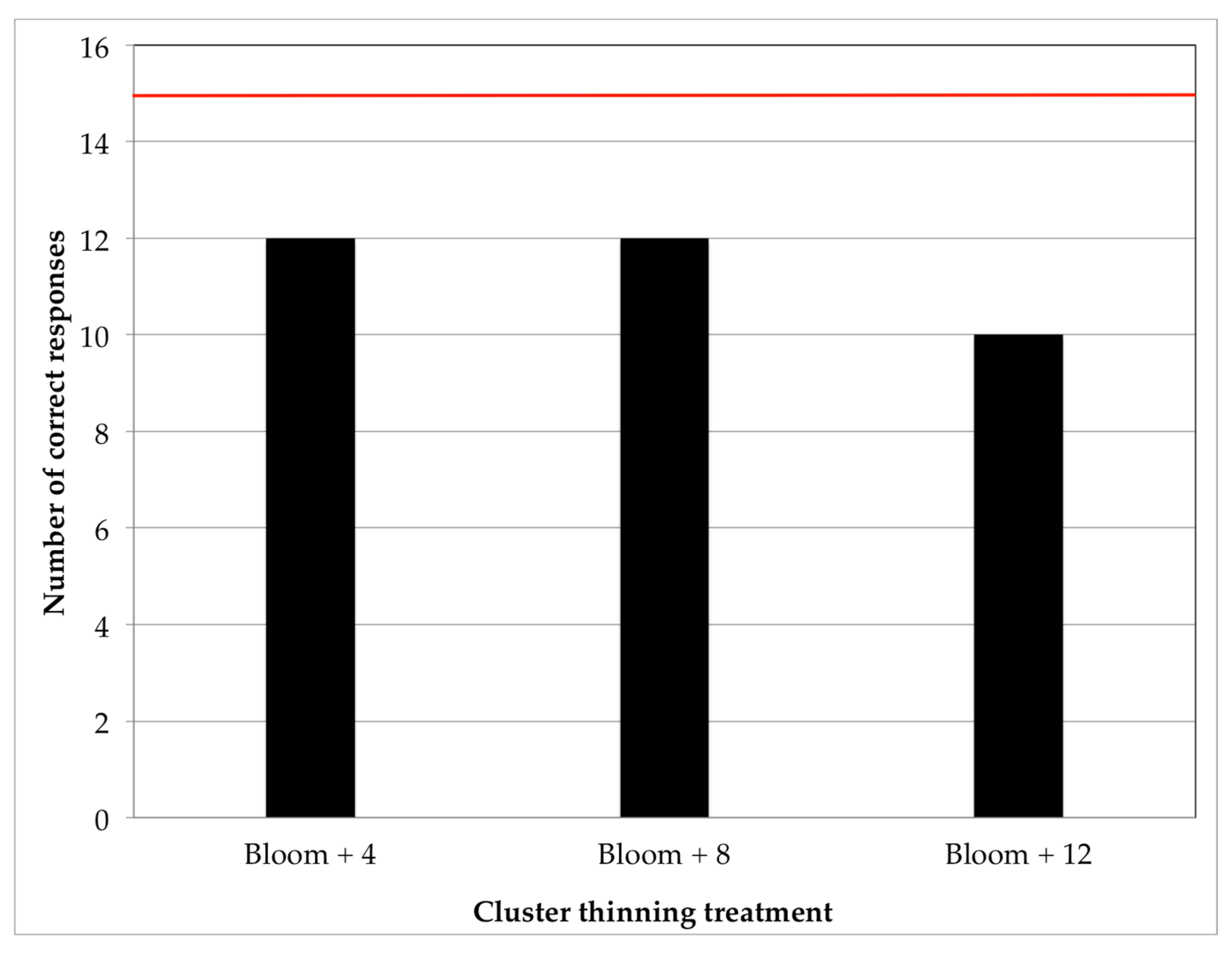
The results of the overall sensory test performed in the 2016 wines generally mirrored previously uncovered trends in the basic, phenolic, and chromatic composition of the resulting wines. That is, none of the cluster thinning treatments produced wines that were distinguishable, from a sensory standpoint, from the control wines. Similar to what has been found in the present study, cluster thinning performed in Chardonnay Musqué grapes, while producing chemical differences in fruit, resulted in little sensory differences in the resulting wines [27]. In another study, wine produced from cluster thinned Cabernet Sauvignon vines exhibited a small increase in perceived wine quality relative to wine produced from non-thinned vines [40], although location was found to have a greater impact on sensory perception than the cluster thinning treatment, and the effect was not consistent across growing seasons. While wine chemical composition and perceived sensory attributes rarely follow linear correlations, without corresponding differences in chemical composition, it is unlikely that cluster thinning will have an impact on wine sensory perception. Therefore, the lack of sensory differences observed in the wines of the present study is unsurprising, and we hypothesize that any chemical differences in volatiles that may have occurred within the wines were below sensory thresholds, and therefore practically irrelevant. Unless cluster thinning is necessitated by the vine balance (i.e., the vine is overcropped) in cool climate Pinot noir, it is unlikely that there will be any sensory benefit to cluster thinning that would justify the negative economic impact associated with cluster thinning.

In much of the previous research performed on cluster thinning, external factors independent of (although at times in combination with) vine crop load impacted berry and wine chemical composition to a greater degree than crop load. Factors such as climatic variation in growing season [21] and viticultural practices such as floor management [34], deficit irrigation [21,22], and leaf thinning [74,75] have all been found to have a greater effect on fruit composition than cluster thinning. Indeed, in the present study, no consistent effect of cluster thinning or cluster thinning timing was observed across two growing seasons, a cooler growing season and a warmer growing season. Conversely, the growing season had a greater effect on variation in fruit and wine composition than thinning treatment for most parameters. A Ravaz Index range of 3 to 6 has been previously proposed as an optimum crop load for Pinot noir grown in cool-climates [30]. Based on the lack of differences observed in fruit Brix accumulation, wine composition, and wine sensory perception, Pinot noir vineyards on the central coast of California can, barring climatic conditions severely increasing crop set or severely limiting ripening potential, likely support higher crop levels than those of the vineyard utilized in this this study, which had Ravaz Index values of 3.23 across the non-thinned blocks. Considering previously proposed ranges and the results of the current study, a Ravaz Index value of 6 could be appropriate for Pinot noir on the central coast of California, and should be examined and evaluated accordingly in future work.

5. Conclusions

No positive effect of cluster thinning or the timing of it was observed across two growing seasons, a cooler growing season and a warmer growing season, for Pinot noir grapes and wines. In general, the growing season had a greater effect on variation than thinning treatment for most parameters. Few treatment × growing season interactions were found in wine composition parameters, indicating that rather than cluster thinning treatment being affected by seasonal variation, which has been reported previously, seasonal variation itself was the primary driver of differences in fruit and wine composition. No sensory differences were detected between the non-thinned control and any wines from cluster thinned treatments. However, on average, cluster thinning was associated with a 44% reduction in crop yields, and this reduction in crop load failed to produce a positive or discernible sensory effect on the resulting wines. Pinot noir vineyards on the central coast of California can support crop loads that result in Ravaz Index values larger than 3.23 and potentially up to 6 without concern for impacting ripening potential, barring a severe decrease in GDD accumulation. This study also suggests that in Pinot noir, balanced canopies with LA/Y ratios in tune with the prevalent seasonal conditions of the region would most likely yield quality fruit, with no discernible or marginal improvements in quality due to cluster thinning.

References

1. Harbertson, J.F.; Hodgins, R.E.; Thurston, L.N.; Schaffer, L.J.; Reid, M.S.; Landon, J.L.; Ross, C.F.; Adams, D.O. Variability of tannin concentration in red wines. Am. J. Enol. Vitic. 2008, 59, 210–214. [Google Scholar]
2. Dimitrovska, M.; Bocevska, M.; Dimitrovski, D.; Murkovic, M. Anthocyanin composition of Vranec, Cabernet Sauvignon, Merlot and Pinot Noir grapes as indicator of their varietal differentiation. Eur. Food Res. Technol. 2011, 232, 591–600. [Google Scholar] [CrossRef]
3. Waterhouse, A.L. Wine phenolics. Ann. N. Y. Acad. Sci. 2002, 957, 21–36. [Google Scholar] [CrossRef] [PubMed]
4. Boulton, R. The Copigmentation of Anthocyanins and Its Role in the Color of Red Wine: A Critical Review. Am. J. Enol. Vitic. 2001, 52, 67–87. [Google Scholar]
5. Jordheim, M.; Fossen, T.; Andersen, Ø.M. Characterization of Hemiacetal Forms of Anthocyanidin 3-O -β-Glycopyranosides. J. Agric. Food Chem. 2006, 54, 9340–9346. [Google Scholar] [CrossRef] [PubMed]
6. Bimpilas, A.; Panagopoulou, M.; Tsimogiannis, D.; Oreopoulou, V. Anthocyanin copigmentation and color of wine: The effect of naturally obtained hydroxycinnamic acids as cofactors. Food Chem. 2016, 197, 39–46. [Google Scholar] [CrossRef] [PubMed]
7. Poncet-Legrand, C.; Gautier, C.; Cheynier, V.; Imberty, A. Interactions between flavan-3-ols and poly(l-proline) studied by isothermal titration calorimetry: Effect of the tannin structure. J. Agric. Food Chem. 2007, 55, 9235–9240. [Google Scholar] [CrossRef] [PubMed]
8. Casassa, L.F.; Harbertson, J.F. Extraction, Evolution, and Sensory Impact of Phenolic Compounds during Red Wine Maceration. Annu. Rev. Food Sci. Technol. 2014, 5, 83–109. [Google Scholar] [CrossRef] [PubMed]
9. Lesschaeve, I.; Noble, A.C. Polyphenols: Factors influencing their sensory properties and their effects on food and beverage preferences. Am. J. Clin. Nutr. 2005, 81, 330S–335S. [Google Scholar] [CrossRef] [PubMed]
10. Harbertson, J.F.; Parpinello, G.P.; Heymann, H.; Downey, M.O. Impact of exogenous tannin additions on wine chemistry and wine sensory character. Food Chem. 2012, 131, 999–1008. [Google Scholar] [CrossRef]
11. Ferrer-Gallego, R.; Hernández-Hierro, J.M.; Rivas-Gonzalo, J.C.; Escribano-Bailón, M.T. Sensory evaluation of bitterness and astringency sub-qualities of wine phenolic compounds: Synergistic effect and modulation by aromas. Food Res. Int. 2014, 62, 1100–1107. [Google Scholar] [CrossRef]
12. Villamor, R.R.; Evans, M.A.; Mattinson, D.S.; Ross, C.F. Effects of ethanol, tannin and fructose on the headspace concentration and potential sensory significance of odorants in a model wine. Food Res. Int. 2013, 50, 38–45. [Google Scholar] [CrossRef]
13. Danilewicz, J. Review of Reaction Mechanisms of Oxygen and Proposed Intermediate Reduction Products in Wine: Central Role of Iron and Copper. Am. J. Enol. Vitic. 2003, 54, 73–85. [Google Scholar]
14. Fulcrand, H.; Dueñas, M.; Salas, E.; Cheynier, V. Phenolic reactions during winemaking and aging. Am. J. Enol. Vitic. 2006, 57, 289–297. [Google Scholar]
15. Cliff, M.A.; King, M.C.; Schlosser, J. Anthocyanin, phenolic composition, colour measurement and sensory analysis of BC commercial red wines. Food Res. Int. 2007, 40, 92–100. [Google Scholar] [CrossRef]
16. Van Buren, J.; Bertino, J. The stability of wine anthocyanins on exposure to heat and light. Am. J. Enol. Vitic. 1968, 19, 147–154. [Google Scholar]
17. Brouillard, R.; Chassaing, S.; Fougerousse, A. Why are grape/fresh wine anthocyanins so simple and why is it that red wine color lasts so long? Phytochemistry 2003, 64, 1179–1186. [Google Scholar] [CrossRef]
18. Somers, T.C.; Evans, M.E. Wine quality: Correlations with colour density and anthocyanin equilibria in a group of young red wines. J. Sci. Food Agric. 1974, 25, 1369–1379. [Google Scholar] [CrossRef]
19. Reynolds, A.G.; Price, S.F.; Wardle, D.A.; Watson, B.T. Fruit Environment and Crop Level Effects on Pinot-Noir. 1. Vine Performance and Fruit Composition in British-Columbia. Am. J. Enol. Vitic. 1994, 45, 452–459. [Google Scholar]
20. Guidoni, S.; Allara, P.; Schubert, A. Effect of cluster thinning on berry skin anthocyanin composition of Vitis vinifera cv. Nebbiolo. Am. J. Enol. Vitic. 2002, 53, 224–226. [Google Scholar]
21. Keller, M.; Mills, L.J.; Wample, R.L.; Spayd, S.E. Cluster Thinning Effects on Three Deficit-Irrigated Vitis vinifera Cultivars. Am. J. Enol. Vitic. 2005, 56, 91–103. [Google Scholar] [CrossRef]
22. Valdés, M.E.; Moreno, D.; Gamero, E.; Uriarte, D.; Prieto, M.D.H.; Manzano, R.; Picon, J.; Intrigliolo, D.S. Effects of cluster thinning and irrigation amount on water relations, growth, yield and fruit and wine composition of tempranillo grapes in extremadura (Spain). J. Int. Sci. Vigne Vin 2009, 43, 67–76. [Google Scholar]
23. Santesteban, L.G.; Miranda, C.; Royo, J.B. Thinning intensity and water regime affect the impact cluster thinning has on grape quality. Vitis J. Grapevine Res. 2011, 50, 159–165. [Google Scholar]
24. Gamero, E.; Moreno, D.; Talaverano, I.; Prieto, M.H.; Guerra, M.T.; Valdés, M.E. Effects of irrigation and cluster thinning on tempranillo grape and wine composition. S. Afr. J. Enol. Vitic. 2014, 35, 196–204. [Google Scholar] [CrossRef]
25. Uzes, D.; Skinkis, P.A. Factors Influencing Yield Management of Pinot Noir Vineyards in Oregon. J. Ext. 2016, 54, 2012–2014. [Google Scholar]
26. Palliotti, A.; Cartechini, A. Cluster thinning effects on yield and grape composition in different grapevine cultivars. Acta Hortic. 2000, 512, 111–119. [Google Scholar] [CrossRef]
27. Reynolds, A.G.; Schlosser, J.; Sorokowsky, D.; Roberts, R.; Willwerth, J.; De Savigny, C. Magnitude of viticultural and enological effects. II. Relative impacts of cluster thinning and yeast strain on composition and sensory attributes of Chardonnay Musqué. Am. J. Enol. Vitic. 2007, 58, 25–41. [Google Scholar] [CrossRef]
28. Bravdo, B.; Hepner, Y.; Loinger, C.; Cohen, S.; Tabacman, H. Effect of Crop Level and Crop Load on Growth, Yield, Must and Wine Composition, and Quality of Cabernet Sauvignon. Am. J. Enol. Vitic. 1985, 36, 125–131. [Google Scholar]
29. Jackson, D.I.; Lombard, P.B.; Kabinett, L.Q. Environmental and management practices affecting grape composition and wine quality—A review. Am. J. Enol. Vitic. 1993, 44, 409–430. [Google Scholar]
30. Kliewer, W.M.; Dokoozlian, N.K. Leaf area/crop weight ratios of grapevines: Influence on fruit composition and wine quality. Am. J. Enol. Vitic. 2005, 56, 170–181. [Google Scholar]
31. Ravaz, L. Sur la brunissure de la vigne. C. R. Acad. Sci. 1903, 136, 1276–1278. [Google Scholar]
32. Smart, R.E.; Dick, J.K.; Gravett, I.M.; Fisher, B.M. Canopy management to improve grape yield and wine quality principles and practices. S. Afr. J. Enol. Vitic. 1990, 11, 3–17. [Google Scholar] [CrossRef]
33. Frioni, T.; Zhuang, S.; Palliotti, A.; Sivilotti, P.; Falchi, R.; Sabbatini, P. Leaf removal and cluster thinning efficiencies are highly modulated by environmental conditions in cool climate viticulture. Am. J. Enol. Vitic. 2017, 68, 325–335. [Google Scholar] [CrossRef]
34. Reeve, A.L.; Skinkis, P.A.; Vance, A.J.; McLaughlin, K.R.; Tomasino, E.; Lee, J.; Tarara, J.M. Vineyard Floor Management and Cluster Thinning Inconsistently Affect ‘Pinot noir’ Crop Load, Berry Composition, and Wine Quality. HortScience 2018, 53, 318–328. [Google Scholar] [CrossRef]
35. Moreno Luna, L.H.; Reynolds, A.G.; Di Profio, F. Crop Level and Harvest Date Impact Composition of Four Ontario Winegrape Cultivars. I. Yield, Fruit, and Wine Composition. Am. J. Enol. Vitic. 2017, 68, 431–446. [Google Scholar] [CrossRef]
36. Howell, G.S. Sustainable grape productivity and the growth-yield relationship: A review. Am. J. Enol. Vitic. 2001, 52, 165–174. [Google Scholar]
37. Bergqvist, J.; Dokoozlian, N.; Ebisuda, N. Sunlight exposure and temperature effects on berry growth and composition of Cabernet Sauvignon and Grenache in the Central San Joaquin Valley of California. Am. J. Enol. Vitic. 2001, 52, 1–7. [Google Scholar]
38. Cañón, P.M.; González, Á.S.; Alcalde, J.A.; Bordeu, E. Composición fenólica del vino tinto: Efecto de chapoda de brotes y raleo de racimos. Cienc. Investig. Agrar. 2014, 41, 235–248. [Google Scholar] [CrossRef]
39. Gil-Muñoz, R.; Moreno-Pérez, A.; Vila-López, R.; Fernández-Fernández, J.I.; Martínez-Cutillas, A.; Gómez-Plaza, E. Influence of low temperature prefermentative techniques on chromatic and phenolic characteristics of Syrah and Cabernet Sauvignon wines. Eur. Food Res. Technol. 2009, 228, 777–788. [Google Scholar] [CrossRef]
40. Ough, C.S.; Nagaoka, R. Effect of Cluster Thinning and Vineyard Yields on Grape and Wine Composition and Wine Quality of Cabernet Sauvignon. Am. J. Enol. Vitic. 1984, 35, 30–34. [Google Scholar]
41. Freeman, B.M.; Kliewer, A.W.M. Effect of Irrigation, Crop Level and Potassium Fertilization on Carignane Vines. II. Grape and Wine Quality. Am. J. Enol. Vitic. 1983, 34, 197–207. [Google Scholar]
42. Dayer, S.; Prieto, J.A.; Galat, E.; Perez Peña, J. Carbohydrate reserve status of Malbec grapevines after several years of regulated deficit irrigation and crop load regulation. Aust. J. Grape Wine Res. 2013, 19, 422–430. [Google Scholar] [CrossRef]
43. Naor, A.; Gal, Y.; Bravdo, B. Crop load affects assimilation rate, stomatal conductance, stem water potential and water relations of field-grown Sauvignon blanc grapevines. J. Exp. Bot. 1997, 48, 1675–1680. [Google Scholar] [CrossRef] [Green Version]
44. Matthews, M.A.; Nuzzo, V. Berry size and yield paradigms on grapes and wines quality. Acta Hortic. 2007, 754, 423–436. [Google Scholar] [CrossRef]
45. California Grape Acreage Report 2012; California Department of Food and Agriculture: Sacramento, CA, USA, 2013. Available online: https://www.nass.usda.gov/Statistics_by_State/California/Publications/Specialty_and_Other_Releases/Grapes/Acreage/2013/201303grpac.pdf (accessed on 16 June 2018).
46. Settevendemie, M. San Luis Obispo County Department of Agriculture/Weights and Measures Annual Report; County Government Center: San Luis Obispo, CA, USA, 2016.
47. Coombe, B. Growth Stages of the Grapevine: Adoption of a system for identifying grapevine growth stages. Aust. J. Grape Wine Res. 1995, 1, 104–110. [Google Scholar] [CrossRef]
48. Winkler, A.J.; Cook, J.A.; Kliewer, W.M.; Lider, L.A. General Viticulture. Soil Sci. 1975, 120, 462. [Google Scholar] [CrossRef]
49. Harbertson, J.F.; Picciotto, E.A.; Adams, D.O. Measurement of Polymeric Pigments in Grape Berry Extracts and Wines Using a Protein Precipitation Assay Combined with Bisulfite Bleaching. Am. J. Enol. Vitic. 2003, 54, 301–306. [Google Scholar]
50. Harbertson, J.F.; Kennedy, J.A.; Adams, D.O. Tannin in Skins and Seeds of Cabernet Sauvignon, Syrah, and Pinot noir Berries during Ripening. Am. J. Enol. Vitic. 2002, 53, 54–59. [Google Scholar]
51. Meilgaard, M.; Carr, B.; Civille, G. Sensory Evaluation Techniques; CRC Press: Boca Raton, FL, USA, 2006; p. 388. [Google Scholar]
52. Kliewer, W.M. Berry composition of Vitis vinifera cultivars as influenced by photo- and nycto-temperatures during maturation. J. Am. Soc. Hortic. Sci. 1973, 98, 153–159. [Google Scholar]
53. Reeve, A.L.; Skinkis, P.A.; Vance, A.J.; Lee, J.; Tarara, J.M. Vineyard floor management influences “Pinot noir” vine growth and productivity more than cluster thinning. HortScience 2016, 51, 1233–1244. [Google Scholar] [CrossRef]
54. McIntyre, G.N.; Kliewer, W.M.; Lider, L.A. Some Limitations of the Degree Day System as Used in Viticulture in California. Am. J. Enol. Vitic. 1987, 38, 128–132. [Google Scholar]
55. Dokoozlian, N.K.; Kliewer, W.M. Influence of Light on Grape Berry Growth and Composition Varies during Fruit Development. J. Am. Soc. Hortic. Sci. 1996, 121, 869–874. [Google Scholar]
56. Price, S.F.; Breen, P.J.; Valladao, M.; Watson, B.T. Cluster Sun Exposure and Quercetin in Pinot noir Grapes and Wine. Am. J. Enol. Vitic. 1995, 46, 187–194. [Google Scholar]
57. Rienth, M.; Torregrosa, L.; Sarah, G.; Ardisson, M.; Brillouet, J.; Romieu, C. Temperature desynchronizes sugar and organic acid metabolism in ripening grapevine fruits and remodels their transcriptome. BMC Plant Biol. 2016, 16, 164. [Google Scholar] [CrossRef] [PubMed]
58. Boban, N.; Tonkic, M.; Budimir, D.; Modun, D.; Sutlovic, D.; Punda-Polic, V.; Boban, M. Antimicrobial Effects of Wine: Separating the Role of Polyphenols, pH, Ethanol, and Other Wine Components. J. Food Sci. 2010, 75, M322–M326. [Google Scholar] [CrossRef] [PubMed]
59. Singleton, V.L. Oxygen with Phenols and Related Reactions in Musts, Wines, and Model Systems: Observations and Practical Implications. Am. J. Enol. Vitic. 1987, 38, 69–77. [Google Scholar]
60. Guerzoni, M.E.; Sinigaglia, M.; Gardini, F.; Ferruzzi, M.; Torriani, S. Effects of pH, Temperature, Ethanol, and Malate Concentration on Lactobacillus plantarum and Leuconostoc oenos: Modelling of the Malolactic Activity. Am. J. Enol. Vitic. 1995, 46, 368–374. [Google Scholar]
61. Ough, C.S.; Amerine, M.A. Studies with Controlled Fermentation X. Effect of Fermentation Temperature on Some Volatile Compounds in Wine. Am. J. Enol. Vitic. 1967, 18, 157–164. [Google Scholar]
62. Du, G.; Zhan, J.; Li, J.; You, Y.; Zhao, Y.; Huang, W. Effect of Fermentation Temperature and Culture Medium on Glycerol and Ethanol during Wine Fermentation. Am. J. Enol. Vitic. 2012, 63. [Google Scholar] [CrossRef]
63. Coombe, B.G. The Development of Fleshy Fruits. Annu. Rev. Plant Physiol. 1976, 27, 207–228. [Google Scholar] [CrossRef]
64. Kliewer, W.M. Effect of High Temperatures during the Bloom-Set Period on Fruit-Set, Ovule Fertility, and Berry Growth of Several Grape Cultivars. Am. J. Enol. Vitic. 1977, 28, 215–222. [Google Scholar]
65. Gillaspy, G. Fruits: A Developmental Perspective. Plant Cell Online 1993, 5, 1439–1451. [Google Scholar] [CrossRef] [PubMed] [Green Version]
66. Van Volkenburgh, E. Leaf expansion—An integrating plant behaviour. Plant Cell Environ. 1999, 22, 1463–1473. [Google Scholar] [CrossRef]
67. Mullins, M.G.; Bouquet, A.; Williams, L.E. Biology of the Grapevine; Cambridge University Press: Cambridge, UK, 1992; ISBN 0-521-30507-1. [Google Scholar]
68. Jurd, L. Review of Polyphenol Condensation Reactions and their Possible Occurrence in the Aging of Wines. Am. J. Enol. Vitic. 1969, 20, 191–195. [Google Scholar]
69. Chris Somers, T.; Evans, M.E. Spectral evaluation of young red wines: Anthocyanin equilibria, total phenolics, free and molecular SO2, “chemical age”. J. Sci. Food Agric. 1977, 28, 279–287. [Google Scholar] [CrossRef]
70. Casassa, L.F. Flavonoid Phenolics in Red Winemaking. In Phenolic Compunds—Natural Sources, Importance and Applications; Soto-Hernandez, M., Ed.; 2017; pp. 153–196. Available online: https://www.intechopen.com/books/phenolic-compounds-natural-sources-importance-and-applications/flavonoid-phenolics-in-red-winemaking (accessed on 6 June 2018).
71. Heredia, F.J.; Francia-Aricha, E.M.; Rivas-Gonzalo, J.C.; Vicario, I.M.; Santos-Buelga, C. Chromatic characterization of anthocyanins from red grapes—I. pH effect. Food Chem. 1998, 63, 491–498. [Google Scholar] [CrossRef]
72. Weber, F.; Greve, K.; Durner, D.; Fischer, U.; Winterhalter, P. Sensory and Chemical Characterization of Phenolic Polymers from Red Wine Obtained by Gel Permeation Chromatography. Am. J. Enol. Vitic. 2013, 64, 15–25. [Google Scholar] [CrossRef]
73. Casassa, L.F.; Larsen, R.C.; Beaver, C.W.; Mireles, M.S.; Keller, M.; Riley, W.R.; Smithyman, R.; Harbertson, J.F. Sensory Impact of Extended Maceration and Regulated Deficit Irrigation on Washington State Cabernet Sauvignon Wines. Am. J. Enol. Vitic. 2013, 64, 505–514. [Google Scholar] [CrossRef] [Green Version]
74. Girard, B.; Kopp, T.G.; Reynolds, A.G.; Cliff, M. Influence of vinification treatments on aroma constituents and sensory descriptors of Pinot noir wines. Am. J. Enol. Vitic. 1997, 48, 198–206. [Google Scholar]
75. Bubola, M.; Sivilotti, P.; Poni, S. Early leaf removal has a larger effect than cluster thinning on grape phenolic composition in cv. teran grape phenolic composition. Am. J. Enol. Vitic. 2017, 68, 234–242. [Google Scholar] [CrossRef]
Figure 1. Results of the duo-trio test with constant reference performed in the 2016 wines. Each cluster thinning treatment was contrasted against the control treatment. A total of 15 correct responses were needed for a statistically distinguishable sensory difference (p < 0.05). The horizontal red line indicates the number of correct responses required to attain statistical significance.
Fermentation 04 00060 g001