
Using Vegetation near CO2 Mediated Enhanced Oil Recovery (CO2-EOR) Activities for Monitoring Potential Emissions and Ecological Effects

Abstract
:
1. Introduction
2. Material and Methods
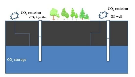
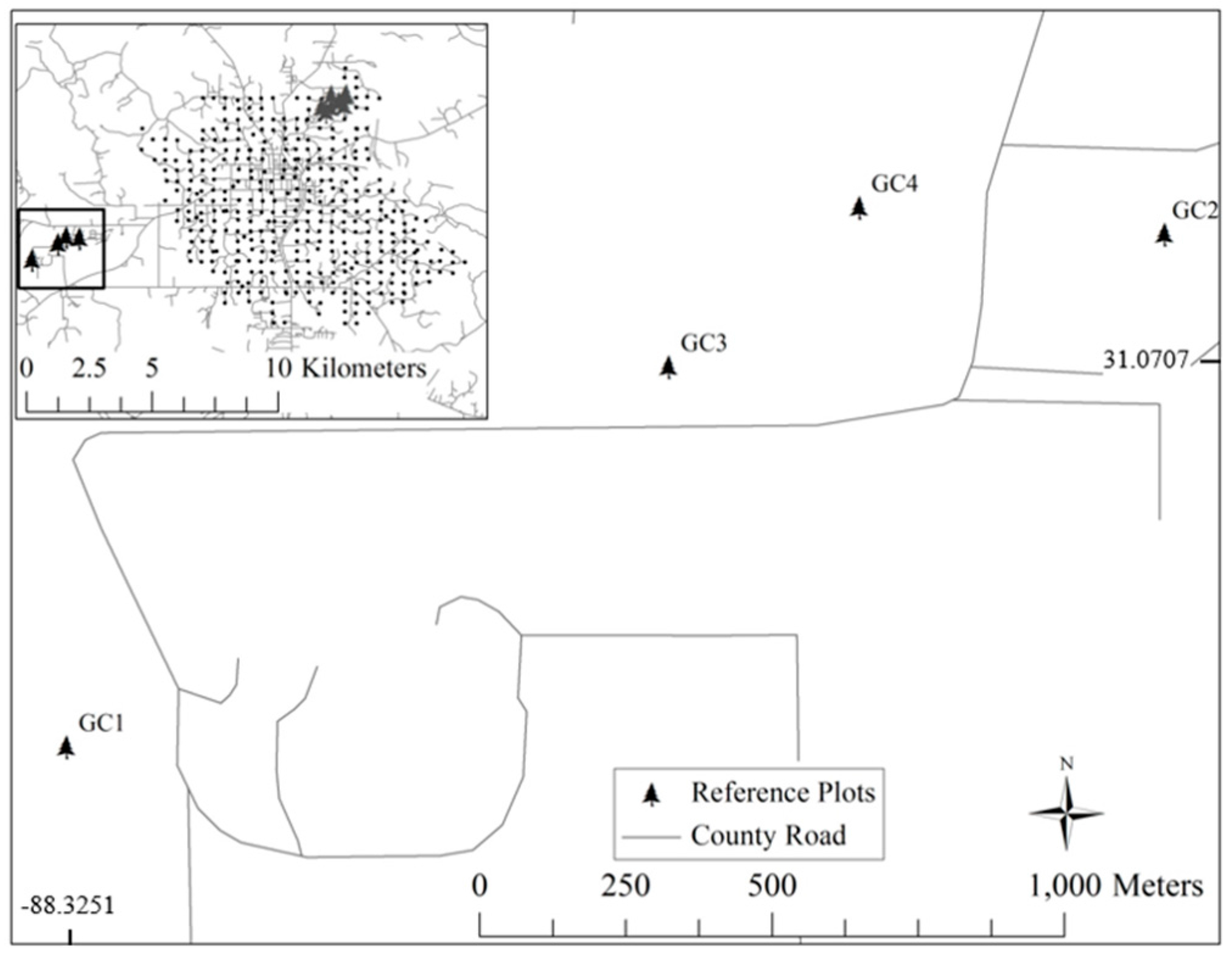
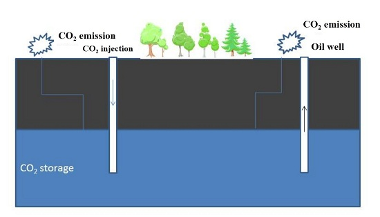
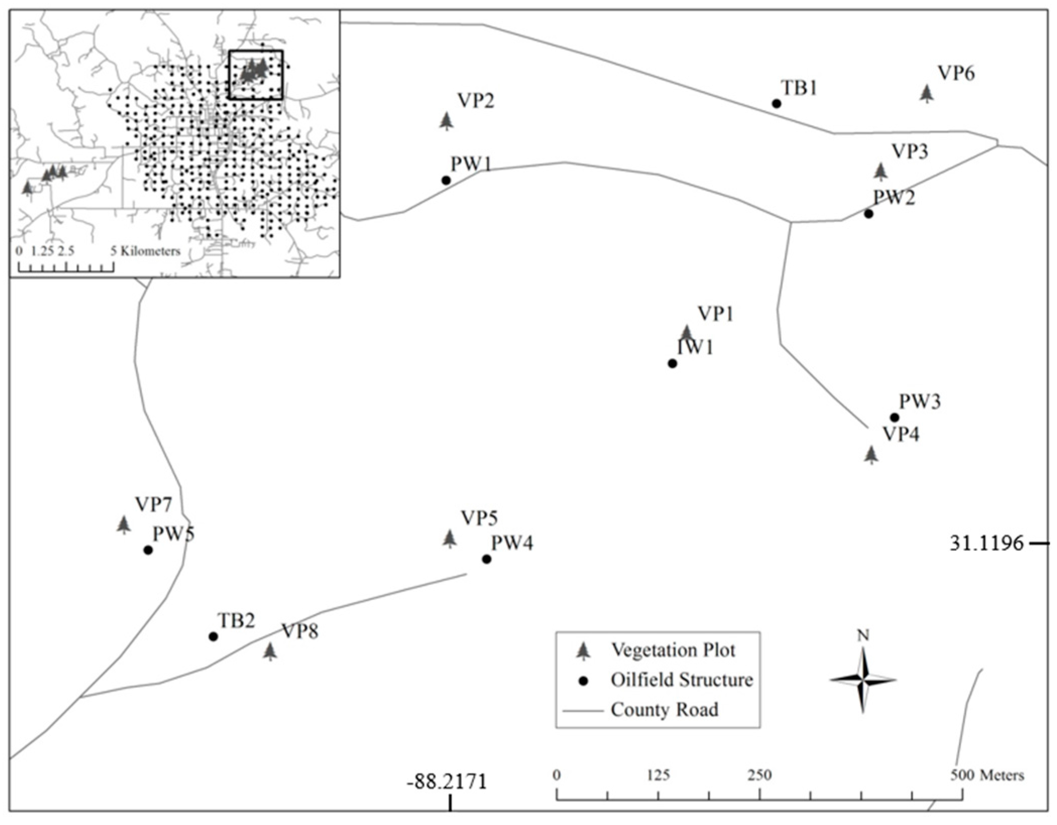
2.1. Study Description

2.2. Vegetation Plots and Direct Measurement
2.3. Data Analysis and Statistics

| Plot | 2009 | 2010 | 2011 |
|---|---|---|---|
| VP2 | 14 | 12 | 12 |
| VP3 | 15 | 12 | 12 |
| VP4b | - | 9 | 12 |
| VP5 | 15 | 12 | 12 |
| VP6 | 15 | 12 | 12 |
| VP7 | 12 | 12 | 12 |
| VP8 | 12 | 12 | 12 |
| GC1 | - | 6 | 12 |
| GC2 | - | 6 | 12 |
| GC3 | - | 6 | 12 |
| GC4 | - | 6 | 12 |
3. Results
| Common Name | Latin Name | VP2 | VP3 | VP4b | VP5 | VP6 | VP7 | VP8 | GC1 | GC2 | GC3 | GC4 |
|---|---|---|---|---|---|---|---|---|---|---|---|---|
| Swamp maple | Acer rubrum spp. | 4 | ||||||||||
| Beech | American Fagus grandifolia | 3 | ||||||||||
| Pawpaw | Asimina triloba | 3 | 2 | |||||||||
| Mockernut | Carya tomentosa (Poir.) Nutt. | 6 | 5 | 1 | ||||||||
| Dogwood | Cornus florida | 5 | 2 | |||||||||
| Leatherwood | Cyrilla racemiflora | 63 | ||||||||||
| Persimmon | Diospyros virginiana | 13 | 3 | 8 | 5 | |||||||
| Huckleberry | Gaylussacia frondosa | 5 | 1 | 2 | 1 | 1 | 4 | |||||
| Carolina holly | Ilex ambigua | 34 | 2 | 2 | 25 | 26 | 28 | |||||
| Holly sp. | Ilex sp. | 12 | ||||||||||
| Winterberry holly | Ilex verticillata | 2 | ||||||||||
| Yaupon holly | Ilex vomitoria | 11 | 28 | 21 | 49 | 9 | 2 | 12 | 45 | 11 | ||
| Eastern Redcedar | Juniperus virginiana L. | 1 | ||||||||||
| Poplar | Liriodendron tulipifera L. | 9 | ||||||||||
| Magnolia | Magnolia grandifora L. | 1 | ||||||||||
| Sweetbay | Magnolia virginiana | 4 | ||||||||||
| Blackgum | Nyssa sylvatica | |||||||||||
| American olive | Osmanthus americanus | 3 | 2 | 15 | 1 | |||||||
| Long leaf pine | Pinus palustris Mill. | 85 | 30 | 4 | 12 | |||||||
| Loblolly pine | Pinus taeda L. | 20 | 21 | 30 | 20 | 9 | ||||||
| Plum | Prunus americana Marsh. | 1 | ||||||||||
| White oak | Quercus alba L. | 1 | 2 | 3 | ||||||||
| Turkey oak | Quercus laevis | 7 | 15 | |||||||||
| Laurel oak | Quercus laurifolia | 6 | 1 | 3 | ||||||||
| Overcup oak | Quercus lyrata Walt. | 1 | 1 | |||||||||
| Blackjack oak | Quercus marilandica | 2 | ||||||||||
| Water oak | Quercus nigra L. | 1 | 2 | 4 | 1 | |||||||
| Willow oak | Quercus phellos L. | 1 | 2 | |||||||||
| Black oak | Quercus velutina Lam. | 1 | 4 | 1 | ||||||||
| Sasafras | Sassafras albidum (Nutt.) | 13 | ||||||||||
| Elm sp | Ulmus sp. | 1 | ||||||||||
| Quercus spp. | 9 | 2 | 6 | 2 | 1 | 3 | ||||||
| Total | 104 | 56 | 77 | 59 | 85 | 53 | 39 | 87 | 71 | 109 | 79 |
3.1. Comparison of Relative Growth Rate Ratio before and after Breakthrough (t-Test)

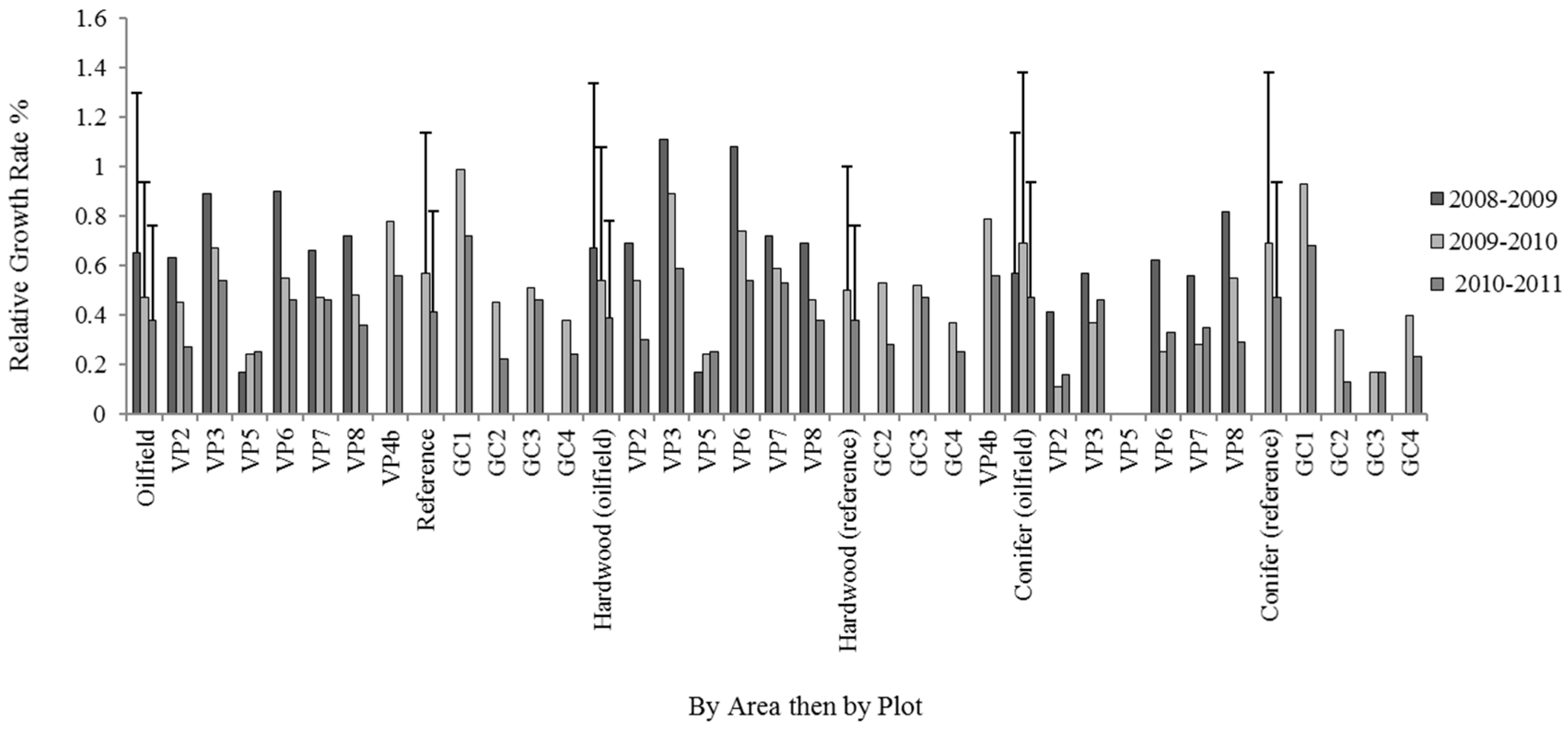
3.2. Oilfield Area (RM-ANOVA)
| Group | F Statistic, p Value | 2008–2009, 2009–2010 | 2009–2010, 2010–2011 | 2008–2009, 2010–2011 | |||
|---|---|---|---|---|---|---|---|
| x̅ ± SD | p Value | x̅ ± SD | p Value | x̅ ± SD | p Value | ||
| Oilfield | F(1.9, 850.7) = 23.34, p ≤ 0.0005 * | 0.58 ± 0.54, 0.44 ± 0.45 | <0.0005 * | 0.44 ± 0.45, 0.38 ± 0.40 | 0.050 * | 0.58 ± 0.54, 0.38 ± 0.40 | <0.0005 * |
| VP1 | F(2, 94) = 9.12, p ≤ 0.0005 * | 0.15 ± 0.22, 0.24 ± 0.33 | 0.388 | 0.24 ± 0.33, 0.44 ± 0.45 | 0.034 * | 0.15 ± 0.22, 0.44 ± 0.45 | <0.0005 * |
| VP2 | F(2, 206) = 19.09, p < 0.0005 * | 0.63 ± 0.49, 0.45 ± 0.42 | 0.019 * | 0.45 ± 0.42, 0.27 ± 0.32 | 0.017 * | 0.63 ± 0.49, 0.27 ± 0.32 | <0.0005 * |
| VP3 | F(2, 110) = 5.38, p = 0.006 * | 0.89 ± 0.67, 0.67 ± 0.57 | 0.228 | 0.67 ± 0.57, 0.54 ± 0.41 | 0.389 | 0.89 ± 0.67, 0.54 ± 0.41 | 0.009 * |
| VP5 | F(1.8, 109.2) = 1.57, p = 0.212 | 0.17 ± 0.23, 0.24 ± 0.29 | 0.225 | 0.24 ± 0.29, 0.25 ± 0.36 | 1.000 | 0.17 ± 0.23, 0.25 ± 0.36 | 0.379 |
| VP6 | F(1.8, 149.5) = 14.10, p ≤ 0.0005 * | 0.90 ± 0.60, 0.55 ± 0.50 | 0.001 * | 0.55 ± 0.50, 0.46 ± 0.47 | 0.547 | 0.90 ± 0.60, 0.46 ± 0.47 | <0.0005 * |
| VP7 | F(2, 104) = 3.72, p = 0.028 * | 0.66 ± 0.41, 0.47 ± 0.49 | 0.139 | 0.47 ± 0.49, 0.46 ± 0.45 | 1.000 | 0.66 ± 0.41, 0.46 ± 0.45 | 0.061 |
| VP8 | F(2, 76) = 5.17, p = 0.008 * | 0.72 ± 0.62, 0.48 ± 0.40 | 0.227 | 0.48 ± 0.40, 0.36 ± 0.30 | 0.464 | 0.72 ± 0.62, 0.36 ± 0.30 | 0.015 * |
3.3. Reference (Paired t-Tests)
3.4. VP4b (Paired t-Tests)
| Reference | 2009–2010 | 2010–2011 | t Statistic | p Value |
|---|---|---|---|---|
| x̅(T2) ± SD | x̅(T3) ± SD | |||
| Total veg | 0.57 ± 0.63 | 0.41 ± 0.46 | t(349) = 4.605 | <0.0005 * |
| GC1 | 0.99 ± 0.58 | 0.72 ± 0.37 | t(85) = 3.247 | 0.002 * |
| GC2 | 0.45 ± 0.49 | 0.22 ± 0.35 | t(72) = 4.286 | <0.0005 * |
| GC3 | 0.51 ± 0.67 | 0.46 ± 0.49 | t(111) = 0.715 | 0.476 |
| GC4 | 0.38 ± 0.62 | 0.24 ± 0.46 | t(78) = 2.266 | 0.026 * |
| Impact-VP4 | 0.78 ± 0.52 | 0.56 ± 0.45 | t(78) = 3.017 | 0.003 * |
3.5. Hardwood Trees
3.6. Coniferous Trees
3.7. Trees

3.8. Shrubs
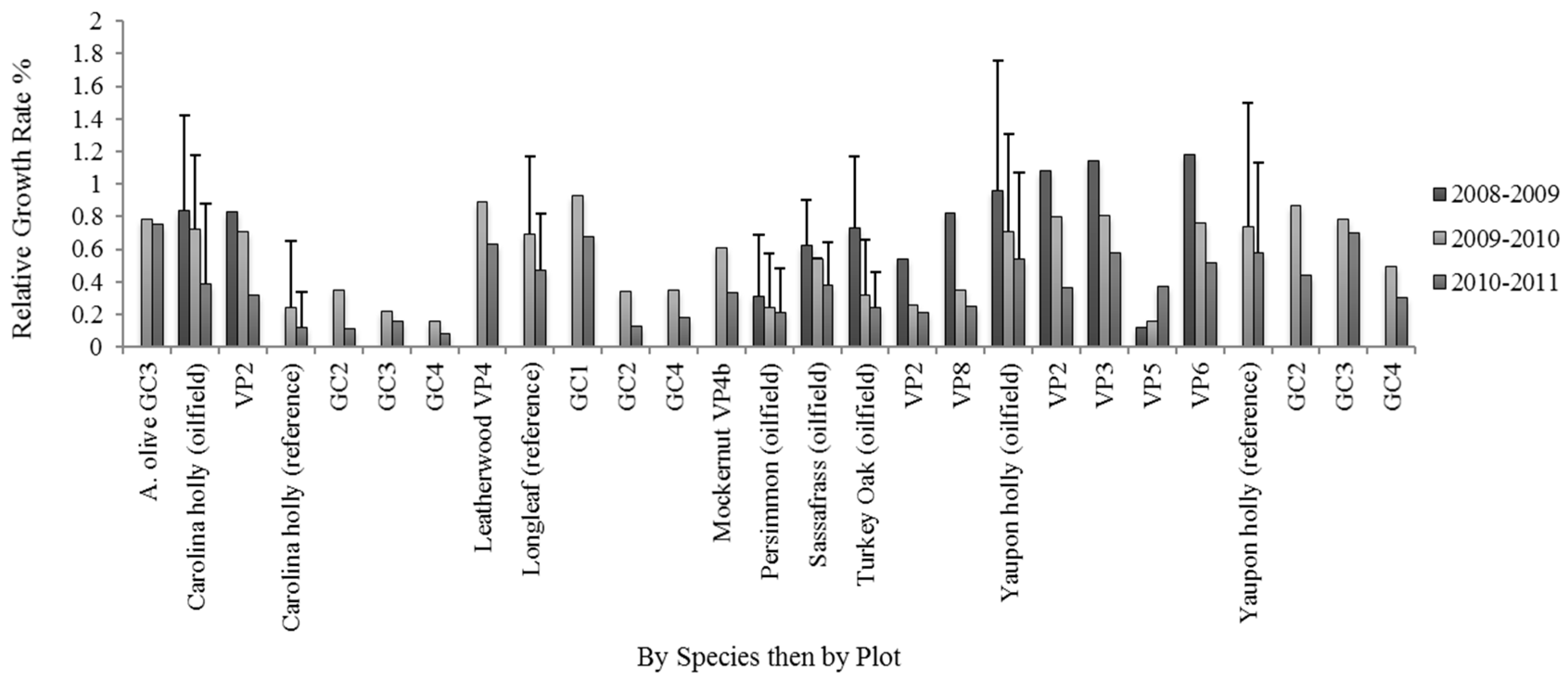
3.9. Species Level

4. Discussion
5. Conclusions
Acknowledgments
Author Contributions
Conflicts of Interest
References
- EIA (Energy Information Administration). AEO 2012 Early Release Overview. Available online: http://205.254.135.7/forecasts/aeo/er/early_fuel.cfm (accessed on 26 October 2015).
- Wildenborg, A.F.B.; van der Meer, L.G.H. The use of oil, gas and coal fields as CO2 sinks. In Proceedings of the IPCC Workshop on Carbon Dioxide Capture and Storage, Regina, Canada, 18–21 November 2002; ECN: Petten, The Netherlands.
- Babadagli, T. Development of mature oil fields—A review. J. Petrol. Sci. Eng. 2007, 57, 221–246. [Google Scholar] [CrossRef]
- Zhang, X.; Xiang, T. Review on microbial enhanced oil recovery technology and development in China. Int. J. Petr. Sci. Tech. 2010, 4, 61–80. [Google Scholar]
- Giacchetta, G.; Leporini, M.; Marchetti, B. Economic and environmental analysis of a Steam Assisted Gravity Drainage (SAGD) facility for oil recovery from Canadian oil sands. Appl. Energy 2015, 142, 1–9. [Google Scholar] [CrossRef]
- Hyne, H.J. Nontechnical guide to petroleum geology, exploration, drilling, and production; Tulsa, PennWell Corporation: Nashua, NH, USA, 2001; pp. 1–598. [Google Scholar]
- Moritis, G. Special report: EOR/Heavy Oil Survey: CO2 miscible, steam dominate enhanced oil recovery processes. Oil Gas J. 2010, 14, 36–53. [Google Scholar]
- Benson, S.; Cook, P.; Anderson, J.; Bachu, S.; Nimir, H.B.; Basu, B.; Bradshaw, J.; Deguchi, G.; Gale, J.; von Goerne, G.; et al. Underground geological storage. In IPCC Special Report on Carbon Dioxide Capture and Storage; Metz, B., Davidson, O., de Coninck, H.C., Loos, M., Meyer, L., Eds.; Cambridge University Press: Cambridge, UK, 2005; pp. 196–276. [Google Scholar]
- Rubin, E.; Meyer, L.; de Coninck, H. Technical summary. In IPCC Special Report on Carbon Dioxide Capture and Storage; Metz, B., Davidson, O., de Coninck, H.C., Loos, M., Meyer, L., Eds.; Cambridge University Press: Cambridge, UK, 2005; pp. 17–50. [Google Scholar]
- ARI. US Oil Production Potential from Accelerated Deployment of Carbon Capture and Storage; Advanced Resources International, Inc: Arlington, VA, USA, 2010. [Google Scholar]
- Leuning, R.; Etheridge, D.; Luhar, A.; Dunse, B. Atmospheric monitoring and verification technologies for CO2 geosequestration. Int. J. Greenh. Gas Con. 2008, 2, 401–414. [Google Scholar] [CrossRef]
- Pruess, K. On leakage from geologic storage reservoirs of CO2. In Proceedings of CO2SC Symposium 2006, Lawrence Berkeley National Laboratory, Berkeley, California, 20–22 March 2006.
- Damen, K.; Faaij, A.; Turkenburg, W. Health safety and environmental risks of underground CO2 storage—Overview of mechanisms and current knowledge. Climatic Change 2006, 74, 289–297. [Google Scholar] [CrossRef]
- Zhang, M.; Bachu, S. Review of integrity of existing wells in relation to CO2 geological storage. What do we know? Int. J. Greenh. Gas Con. 2010, 5, 826–840. [Google Scholar] [CrossRef]
- Dooley, J.J.; Dahowski, R.T.; Davidson, C.L. CO2 driven Enhanced Oil Recovery as A Stepping Stone to What? Report PNNL–19557; Pacific Northwest National Laboratory: Richland, WA, USA, 2010. [Google Scholar]
- NETL (National Energy Technology Laboratory). Monitoring, verification, and accounting of CO2 stored in deep geologic formations. 2009. Available online: www.netl.doe.gov/technologies/carbon_seq/refshelf/MVA_Document.pdf (accessed on 26 October 2015). [Google Scholar]
- Kimball, B.A.; Mauney, J.R.; Nakayama, F.S.; Idso, S.B. Effects of increasing atmospheric carbon dioxide on vegetation. Vegetation 1993, 104–105, 65–75. [Google Scholar] [CrossRef]
- Moore, B.D.; Cheng, S.H.; Sims, D.; Seeman, J.R. The biochemical and molecular basis for photosynthetic acclimation to elevated atmospheric CO2. Plant Cell Environ. 1999, 22, 567–582. [Google Scholar] [CrossRef]
- Pritchard, S.G.; Rodgers, H.; Prior, S.A.; Peterson, C.M. Elevated CO2 and plant structure: a review. Global Change Biol. 1999, 5, 807–837. [Google Scholar] [CrossRef]
- Esposito, R.A.; Pashin, J.C.; Walsh, P.M. Citronelle Dome: A giant opportunity for multi–zone carbon storage and enhanced oil recovery in the Mississippi Interior Salt Basin of Alabama. Environ. Geosci. 2008, 15, 1–10. [Google Scholar] [CrossRef]
- NETL. Best practices for: Terrestrial sequestration of Carbon Dioxide. 2010. Available online: http://www.theclimatehub.com/best-practices-for-terrestrial-sequestration-of-carbon-dioxide (accessed on 18 October 2015).
- Levene, H. Robust tests for equality of variances. In Contributions of Probability and Statistics: Essays in Honor of Harold Hotelling; Olkin, I., Ed.; Stanford University Press: Palo Alto, CA, USA, 1960; pp. 278–292. [Google Scholar]
- Walsh, P.M.; Nyakatawa, E.Z.; Chen, X.; Dittmar, G.N.; Boelens, T.; Donlon, C.; Walker, S.; Guerra, P.; Jolly, R.; Shepherd, D.; et al. Carbon-Dioxide-Enhanced Oil Production from the Citronelle Oil Field in the Rodessa Formation, South Alabama; University of Alabama: Birmingham, AL, USA, 30 April 2011. [Google Scholar]
- Chow, F.K.; Granvold, P.W.; Oldenburg, C.M. Modeling the effects of topography and wind on atmospheric dispersion of CO2 surface leakage at geologic carbon sequestration sites. Energy Procedia 2009, 1, 1925–1932. [Google Scholar] [CrossRef]
- Dodds, K.; Daley, T.; Freifeld, B.; Urosevic, M.; Kepic, A.; Sharma, S. Developing a monitoring and verification plan with reference to the Australian Otway CO2 pilot project. The Leading Edge 2010, 28, 812–818. [Google Scholar] [CrossRef] [Green Version]
© 2015 by the authors. Licensee MDPI, Basel, Switzerland. This article is an open access article distributed under the terms and conditions of the Creative Commons Attribution license ( http://creativecommons.org/licenses/by/4.0/).
Share and Cite
Chen, X.; Roberts, K.A. Using Vegetation near CO2 Mediated Enhanced Oil Recovery (CO2-EOR) Activities for Monitoring Potential Emissions and Ecological Effects. C 2015, 1, 95-111. https://doi.org/10.3390/c1010095
Chen X, Roberts KA. Using Vegetation near CO2 Mediated Enhanced Oil Recovery (CO2-EOR) Activities for Monitoring Potential Emissions and Ecological Effects. C. 2015; 1(1):95-111. https://doi.org/10.3390/c1010095
Chicago/Turabian StyleChen, Xiongwen, and Kathleen A. Roberts. 2015. "Using Vegetation near CO2 Mediated Enhanced Oil Recovery (CO2-EOR) Activities for Monitoring Potential Emissions and Ecological Effects" C 1, no. 1: 95-111. https://doi.org/10.3390/c1010095
APA StyleChen, X., & Roberts, K. A. (2015). Using Vegetation near CO2 Mediated Enhanced Oil Recovery (CO2-EOR) Activities for Monitoring Potential Emissions and Ecological Effects. C, 1(1), 95-111. https://doi.org/10.3390/c1010095