Comparative Performance Assessment between Incompressible and Compressible Solvers to Simulate a Cavitating Wake

Abstract

To study the effects of fluid compressibility on the dynamics of a cavitating vortex street flow in a regime where the vortex shedding frequency increases as a result of the cavitation increase, the cavitating wake behind a wedge was simulated employing both incompressible and compressible solvers. To do this, a compressible cavitation model was implemented, modifying the Zwart-Gerber-Belamri (ZGB) incompressible solver and including a pressure limit and absorbing boundary conditions to prevent a non-physical pressure field. To validate the performance of the compressible model, preliminary simulations were carried out on a 1D Sod cavitating tube and the cavitating vortex shedding behind a circular body at laminar flow conditions. The results of the cavitating wake behind the wedge with the incompressible and the compressible solvers showed similar predictions in terms of pressure, vortex shedding frequency, and instantaneous and average vapor volume fraction profiles. In spite of this, differences were obtained in the energy content of the fluid force fluctuations on the body at higher frequencies, which appear to be better resolved and amplified when the compressibility model is considered. Overall, both solvers provided comparable results in terms of cavitation phenomena that are well aligned with experimental observations.

1. Introduction

Vortical flow structures and cavitation are two common phenomena encountered in hydraulic machinery [1,2,3]. As the fluid passes the fixed vanes, the guide vanes, or the runner blades, it creates complex wake flow patterns that might develop in what is known as a vortex street. The resulting alternating shed vortices induce force fluctuations on the solids and provoke vortex-induced vibrations that may induce severe fatigue damage. In addition, vaporous cavities will be formed and persist inside the center of the alternating shed vortices if the ambient pressure is low enough [4]. As these cavities move to the high-pressure region and collapse, they can also induce severe material erosion on adjacent surfaces. It is well known that the occurrence and development of cavitation can strongly alter the dynamic behavior of vortex street flows [5,6,7,8]. For example, it was reported that cavitation tends to enhance the amplitude of vortex-induced vibrations [7]. Therefore, further exploration of the effect of cavitation on the vortex street flow is essential to mitigate the damage caused by the cavitation and/or vortex-induced vibrations.

Currently, the computational fluid dynamic (CFD) method has been proved to provide detailed insights into complex flow fields, particularly in cases involving cavitation. Various numerical approaches, each with different levels of complexity, are available to simulate cavitating flow. For a comprehensive review of cavitation modeling approaches, see Niedźwiedzka et al. [9] and Folden and Aschmoneit [10]. Among these numerical models, the transport equation model (TEM) is one of the most widely used; this includes an additional transport equation for the vapor phase volume fraction and a source term that accounts for the mass transfer between phases. Without considering fluid compressibility, TEM-based simulations can effectively capture the transition from sheet to cloud cavitation, driven by a liquid re-entrant jet across different geometries [11,12,13], aligning well with experimental observations [1,14,15,16,17]. Conversely, the transition from sheet cavitation to cloud cavitation can be dominated by condensation shock [18,19,20], which is highly related to the fluid compressibility of the mixture. Coupled with the equation of state for the liquid and vapor, TEM can successfully capture the condensation shock and its impact on the transition from sheet cavitation to cloud cavitation [13,20,21,22,23].

For the developed cavitation within the vortex street flows, bubble–vortex interactions alter the growth and collapse dynamics of the cavitation [24,25,26,27,28,29,30]. This makes the roles of fluid compressibility in cavitating vortex street flows distinct from those observed in unsteady cloud cavitation. Previous numerical investigations highlighted the impact of fluid compressibility on cavitating vortex street flows, particularly at extremely low cavitation numbers. For example, Brandao and Mahesh [31] numerically captured the condensation shock on the surface of the circular cylinder where cavitation was highly developed. Additionally, Kim et al. [32] confirmed that fluid compressibility can alter the morphology of fully developed cavities when the cavitation number is less than half of the cavitation inception number. Recently, Wang et al. numerically captured the interaction between the microbubbles and streamwise vortices in cavitating vortex street flow using the Euler–Lagrange method [33]. However, the effects of fluid compressibility on the dynamics of vortex street flows have received limited attention, especially at intermediate cavitation numbers.

The aim of this study is to demonstrate the influence of fluid compressibility on the dynamics of a cavitating vortex street by numerically resolving the cavitating flow field using both incompressible and compressible cavitation solvers. This paper is composed of five sections. Following this introduction, the second section explains the governing equations. The third section details the corresponding numerical treatment. In the fourth section, the implemented numerical solvers are validated, and the results from both the incompressible and compressible solvers are compared. Finally, the fifth section presents the conclusions and summarizes the results.

2. Governing Equations

2.1. Mass Conservation Equation

The equation for the conserved mass without an external mass source is given by:

$$\partial \rho /\partial t+\nabla ·\left(\rho \mathit{u}\right)=0$$

(1)

where $\rho$ is the density, $\mathit{u}$ is the velocity, and $t$ is the time. This equation is valid for both incompressible and compressible flows.

2.2. Momentum Conservation Equation

In an inertial reference frame, the conserved momentum equation can be written as follows:

$$\partial \left(\rho \mathit{u}\right)/\partial t+\nabla ·\left(\rho \mathit{u}⨂\mathit{u}\right)=-\nabla p+\nabla ·\mathit{\tau }$$

(2)

where $p$ is the pressure, and $\mathit{\tau }$ is the stress tensor, which is defined as:

$$\mathit{\tau }=\mu \left[\nabla \mathit{u}+{\nabla \mathit{u}}^T-2/3\left(\nabla ·\mathit{u}\right)\mathit{I}\right]$$

(3)

where $\mu$ is the fluid molecular viscosity, and $\mathit{I}$ is the unit tensor.

2.3. Realizable $k$-Epsilon Delayed Detached Eddy Simulation (DDES) Model

In the realizable $k$-epsilon DDES model, the governing equation for the turbulence kinetic energy, $k$, can be written as follows:

$$\partial \left(\rho k\right)/\partial t+\nabla ·\left(\rho \mathit{u}k\right)=P_k-Y_k^{\mathrm{*}}+\nabla ·\left[\left(\mu +{\mu }_t/{\sigma }_k\right)\nabla k\right]$$

(4)

where $\epsilon$ is the dissipation, $P_k$ is the generation term of $k$, ${\mu }_t$ is the turbulent viscosity, and ${\sigma }_k$ is the turbulent Prandtl number. Furthermore, the dissipation of turbulent kinetic energy, $Y_k^{\mathrm{*}}$, is given by:

$$Y_k^{\mathrm{*}}={\displaystyle \frac{\rho k^{\frac{3}{2}}}{l_{des}}}$$

(5)

where

$$l_{des}=\min \left(l_{rke},l_{les}\right); l_{rke}={\displaystyle \frac{k^{\frac{3}{2}}}{\epsilon }}; l_{les}=C_{des}{\mathsf{\Delta }}_{max}$$

(6)

where $l_{rke}$ and $l_{les}$ are the calculated length scales based on the realizable $k$-epsilon model and LES, respectively. ${\mathsf{\Delta }}_{max}$ is the maximum length of the cell edge, and $C_{des}=0.61$ is the model constant. If $l_{rke}$= $l_{les}$, $l_{des}$ is replaced by the following functions:

$$l_{des}=l_{rke}-f_y\mathrm{m}\mathrm{a}\mathrm{x}\left(0,l_{rke}-C_{des}{\mathsf{\Delta }}_{max}\right)$$

(7)

$$f_y=1-\tan \mathrm{h}\left[{\left(20.0r_y\right)}^3\right]$$

(8)

$$r_y={\displaystyle \frac{\left(\mu +{\mu }_t\right)/\rho }{\sqrt{\mathit{u}:\mathit{u}}\kappa y^2}}$$

(9)

where y represents the wall distance, and κ = 0.41.

2.4. Cavitation Modeling

The volume fraction transport equation for the vapor volume fraction, ${\alpha }_v$, is given by:

$$\partial \left({\rho }_v{\alpha }_v\right)/\partial t+\nabla ·\left({\rho }_v{\alpha }_v\mathit{u}\right)=\dot{m}$$

(10)

The $\rho$ and $\mu$ of the fluid mixture are defined, respectively, as:

$$\rho ={\alpha }_v{\rho }_v+\left(1-{\alpha }_v\right){\rho }_l$$

(11)

$$\mu ={\alpha }_v{\mu }_v+\left(1-{\alpha }_v\right){\mu }_l$$

(12)

where ${\rho }_v$ and ${\rho }_l$ are the water and vapor densities, respectively, and ${\mu }_v$ and ${\mu }_l$ are the water and vapor dynamic viscosities, respectively.

The mass transfer rate between the liquid and vapor due to the cavitation is modeled with a source term, $\dot{m}$, presented in Equation (10). If the effects of viscosity, non-condensable gas, surface tension, and second-order derivation are neglected, the Rayleigh–Plesset equation can be simplified and written as:

$$\dot{R}=\sqrt{{\displaystyle \frac{2\left(P_{ref}-p_v\right)}{3{\rho }_l}}}$$

(13)

where $p$ is the saturated vapor pressure, and $R$ is the bubble radius.

Assuming that the distribution of the nucleation inside the flow field is uniform and independent of the flow structures, then the relationship between the bubble radius, $R$, and ${\alpha }_v$ is given by:

$${\alpha }_v=n_v{\displaystyle \frac{4\pi }{3}}{R}^3$$

(14)

where $n_v$ is the number of nucleations per unit volume. Then, $\dot{m}$ is calculated by:

$$\dot{m}={\rho }_v{\dot{\alpha }}_v=n_v{\rho }_{v}3{\displaystyle \frac{4\pi }{3}}{R}^2\dot{R}$$

(15)

By submitting $n$ given by Equations (13) and (14) into Equation (15), $\dot{m}$ can be expressed as:

$$\dot{m}={\displaystyle \frac{3{\rho }_v{\alpha }_v}{R}}\sqrt{{\displaystyle \frac{2\left(P_{ref}-p_v\right)}{3{\rho }_l}}}$$

(16)

In the vaporization process, the nucleation site density must decrease as the vapor volume fraction increases. To model this process, $\alpha$ needs to be replaced with $\left(1-{\alpha }_v\right){\alpha }_{\mathrm{nuc}}$ in Equation (16). Then, the final ZGB cavitation model [34] is presented as follows:

$$\dot{m}=\left\{\begin{array}{c}{F}_c{\displaystyle \frac{3{\alpha }_v{\rho }_v}{R_0}}\sqrt{{\displaystyle \frac{2}{3}}{\displaystyle \frac{\left(p-p_v\right)}{{\rho }_l}}}p>p_v\\ F_v{\displaystyle \frac{3{\rho }_v\left(1-{\alpha }_v\right){\alpha }_{nuc}}{R_0}}\sqrt{{\displaystyle \frac{2}{3}}{\displaystyle \frac{\left(p_{\mathrm{v}}-p\right)}{{\rho }_l}}}p<p_v\end{array}\right.$$

(17)

where $p_{\mathrm{v}}$ is the saturated vapor pressure. The initial value of the bubble radius is $R_0=1 \mathsf{\mu }\mathrm{m}$, and the nucleation site of the volume fraction ${\alpha }_{\mathrm{nuc}}=5\times {10}^{-4}$. Here, the optimal empirical condensation and vaporization coefficients have been selected as $F_c=0.001$ and $F_v=50.0$, respectively.

2.5. Equation of State

The density of the compressible liquid phase can be computed using the Tait equation [22,35]:

$${\rho \left(p\right)}_l={\rho }_{l,sat}{\left({\displaystyle \frac{p+B}{p_v+B}}\right)}^{1/N}$$

(18)

and the corresponding sound speed is defined as

$${c\left(p\right)}_l=\sqrt{{\displaystyle \frac{\partial p}{\partial \rho }}}=\sqrt{{\displaystyle \frac{N}{{\rho }_{l,sat}}}\left(p_v+B\right){\left({\displaystyle \frac{p+B}{p_v+B}}\right)}^{\left(N-1\right)/N}}$$

(19)

where $B$ is the water bulk modulus, $3.1\times {10}^8$ Pa, ${\rho }_{l,sat}$ is the liquid density at $p_v$, 998.18 kg/m³, and $N$ is a model constant equal to 7.15.

The density of the compressible vapor phase using the polytropic equation of state [36] can be written as:

$${\rho \left(p\right)}_v={\left(p/C_v\right)}^{1/n}$$

(20)

and the corresponding sound speed is:

$${c\left(p\right)}_v=\sqrt{{\displaystyle \frac{\partial p}{\partial \rho }}}=\sqrt{C_{v}n{\left(p/C_v\right)}^{\left(n-1\right)/n}}$$

(21)

where the model constant $C_v$ can be estimated from a density of 0.017 kg/m³ at $p_v$. The polytropic exponent $n$ for an adiabatic assumption is 1.4.

2.6. Sponge Layer Conditions

To date, although the use of the pressure-based method has achieved notable success in a wide range of compressible cavitating flows [37,38], several unresolved numerical difficulties remain, particularly concerning the determination of the inlet and outlet boundary conditions in CFD simulations. Typically, such calculations are conducted on a truncated domain of the entire system, and the standard inlet/outlet boundary conditions may fail to allow some of the flow features to leave the computational domain as physically expected. For that reason, artificial treatments of the truncated domains are required to avoid pressure waves reflected at the boundaries. Therefore, the sponge layer was adopted for its flexibility and simplicity [39]. The set of formulas of the sponge layer, based on the pressure and velocity for the pressure-based method, is given as follows:

$$\partial \rho /\partial t+\nabla ·\left(\rho \mathit{u}\right)=\mathit{\sigma }\left(\mathit{x}\right){\left.{\displaystyle \frac{\partial \rho }{\partial p}}\right|}_{p=p_{ref}}\left(p_{ref}-p\right)$$

(22)

$$\partial \left(\rho \mathit{u}\right)/\partial t+\nabla ·\left(\rho \mathit{u}\mathit{u}+p\mathit{I}-\mathit{\tau }\right)=\mathit{\sigma }\left(\mathit{x}\right)\rho \left({\mathit{u}}_{ref}-\mathit{u}\right)$$

(23)

where the subtitle “ref” refers to a target value of the flow variable, and $\mathit{\sigma }\left(\mathit{x}\right)$ is the function of the damping coefficient, which is defined as:

$$\mathit{\sigma }\left(\mathit{x}\right)={\displaystyle \frac{3{{\alpha }_{pol}\left(\mathit{x}/L\right)}^{{\beta }_{pol}}}{2{∆t}^{{\gamma }_{pol}}}}$$

(24)

where ${\alpha }_{pol}=1.0$, ${\beta }_{pol}=3.0$, ${\gamma }_{pol}=1.0,$ x is the distance from the leading edge of the sponge layer, and $L$ is the length of the sponge layer, as shown in Figure 1.

3. Numerical Method

In this section, the governing equations are discretized using the finite volume method (FVM) over the collocated unstructured mesh. More attention will be paid to the numerical algorithm for the pressure-based multiphase solver with/without consideration of fluid compressibility using a predefined macro inside the ANSYS Fluent 2022R2 platform provided as a Supplementary File.

3.1. Incompressible Mixture/VOF Model

Without consideration of fluid compressibility, the fluid densities are constant. The numerical algorithm for the mass conservation and volume fraction transport equation with linearized source terms is detailed in the following subsection.

3.1.1. Incompressible Volume Continuity Equation

To guarantee mass conservation and numerical stability, the pressure-correction equation is based on the total volume continuity instead of the mass conservation equation.

$${\displaystyle \frac{1}{{\rho }_v}}\left[\partial \left({\rho }_v{\alpha }_v\right)/\partial t+\nabla ·\left({\rho }_v{\alpha }_v\mathit{u}\right)-\dot{m}\right]+{\displaystyle \frac{1}{{\rho }_l}}\left[\partial \left({\rho }_l{\alpha }_l\right)/\partial t+\nabla ·\left({\rho }_l{\alpha }_l\mathit{u}\right)+\dot{m}\right]=0$$

(25)

Integrating Equation (25) over a control volume, the discretized form of the volume continuity is given by:

$$\left\{\begin{array}{c}{\displaystyle \frac{1}{{\rho }_v}}\left({\displaystyle \frac{{\rho }_v{\alpha }_v-{\rho }_v{{\alpha }_v}^0}{∆t}}dV+{\displaystyle \sum _f}{\rho }_v{\alpha }_v{\mathit{u}}_f{\mathit{A}}_f\right)+\\ {\displaystyle \frac{1}{{\rho }_v}}\left({\displaystyle \frac{{\rho }_l{\alpha }_l-{\rho }_l{{\alpha }_l}^0}{∆t}}dV+{\displaystyle \sum _f}{\rho }_l{\alpha }_l{\mathit{u}}_f{\mathit{A}}_f\right)\end{array}\right\}=\left\{\begin{array}{c}\left({\displaystyle \frac{1}{{\rho }_v}}-{\displaystyle \frac{1}{{\rho }_l}}\right)\left[{\dot{m}}^{\mathrm{*}}-{\left({\displaystyle \frac{\partial \dot{m}}{\partial p}}\right)}^{\mathrm{*}}\left(p^{\mathrm{*}}-p_{\mathrm{v}}\right)\right]+\\ \underset{ds/dp}{\underbrace{{\left({\displaystyle \frac{\partial \dot{m}}{\partial p}}\right)}^{\mathrm{*}}\left({\displaystyle \frac{1}{{\rho }_v}}-{\displaystyle \frac{1}{{\rho }_l}}\right)}}\left(p-p_{\mathrm{v}}\right)\end{array}\right\}$$

(26)

where $dV$ is the volume of the control cell, ${\mathit{A}}_f$ is the face area vector within the control volume, and ${\rho }_v{\alpha }_v{\mathit{u}}_f$ and ${\rho }_l{\alpha }_l{\mathit{u}}_f$ are the vapor and liquid mass fluxes, respectively. On the collocated grid, the phase mass flux is computed using a Rhie–Chow interpolation.

More importantly, the term $ds/dp$ is the linearized mass transfer related to the pressure for the pressure correction equation, which can enhance the numerical stability of the cavitation simulation.

3.1.2. Incompressible Second Phase Fraction Equation

In ANSYS Fluent, only the transport equation for the second phase volume fraction is solved using the VOF or mixture model. Normally, the vapor phase is set to be the second phase. Thus, the vapor volume fraction is obtained with the vapor phase continuity equation, as presented in Equation (10). Correspondingly, the discretized form of the equation can be written as follows:

$${\displaystyle \frac{1}{{\rho }_v}}\left({\displaystyle \frac{{\rho }_v{\alpha }_v-{\rho }_v{{\alpha }_v}^0}{∆t}}dV+\sum _f{\rho }_v{\alpha }_v{\mathit{u}}_f{\mathit{A}}_f\right)={\displaystyle \frac{\dot{m}}{{\rho }_v}}dV$$

(27)

Assuming that the mass source term $\dot{m}$ can be rewritten as the function of ${\alpha }_v$ and ${\alpha }_l$:

$${\displaystyle \frac{\dot{m}}{{\rho }_v}}={\dot{m}}_0+S_l{\alpha }_l-S_v{\alpha }_v$$

(28)

With the linearized mass source term $\dot{m}$, the Equation (27) can be rewritten as:

$${\displaystyle \frac{1}{{\rho }_v}}\left({\displaystyle \frac{{\rho }_v{\alpha }_v-{\rho }_v{{\alpha }_v}^0}{∆t}}dV+\sum _f{\rho }_v{\alpha }_v{\mathit{u}}_f{\mathit{A}}_f\right)=\left(S_c+S_p{\alpha }_v\right)dV$$

(29)

where

$$\left\{\begin{array}{c}{S}_c={\dot{m}}_0+S_l\\ S_p=-\left(S_v+S_l\right)\end{array}\right.$$

(30)

where $S_p$ is the linear part of the source term $\dot{m}$, and $S_c$ is the part of $\dot{m}$ that cannot be linearized.

3.2. Compressible Mixture/VOF Model

In this section, the robust numerical algorithm for multiphase flows to handle fluid compressibility is introduced [37]. With the SIMPLE method, velocity and density fields can be decomposed into two parts, as follows:

$$\left\{\begin{array}{c}{\rho }_v=\left({{\rho }_v}^{\mathit{*}}+{{\rho }_v}^{\prime }\right)={{\rho }_v}^{\mathit{*}}+\left({\displaystyle \frac{\partial {{\rho }_v}^{\mathit{*}}}{\partial p}}\right)p^{\prime }\\ {\rho }_l=\left({{\rho }_l}^{\mathit{*}}+{{\rho }_l}^{\prime }\right)={{\rho }_l}^{\mathit{*}}+\left({\displaystyle \frac{\partial {{\rho }_l}^{\mathit{*}}}{\partial p}}\right)p^{\prime }\\ \mathit{u}=\left({\mathit{u}}^{\mathit{*}}+{\mathit{u}}^{\prime }\right)\end{array}\right.$$

(31)

where “$\mathrm{*}$” indicates the tentative values, and “$\prime$” indicates the variable correction.

3.2.1. Compressible Volume Continuity Equation

Unlike the incompressible pressure-correction equation, the phase masses for vapor and liquid, ${\rho }_v{\alpha }_v$ and ${\rho }_l{\alpha }_l$, respectively, and the phase flux terms for vapor and liquid, ${\rho }_v{\alpha }_v\mathit{u}$ and ${\rho }_l{\alpha }_l\mathit{u}$, respectively, are computed with the following equations:

$$\left\{\begin{array}{c}{\rho }_v{\alpha }_v={{\rho }_v}^{\mathbf{*}}{\alpha }_v+\left({\displaystyle \frac{\partial {{\rho }_v}^{\mathbf{*}}}{\partial p}}\right)p^{\prime }{\alpha }_v\\ {\rho }_l{\alpha }_l={{\rho }_l}^{\mathbf{*}}{\alpha }_l+\left({\displaystyle \frac{\partial {{\rho }_l}^{\mathbf{*}}}{\partial p}}\right)p^{\prime }{\alpha }_l\end{array}\right.$$

(32)

$$\left\{\begin{array}{c}{\rho }_v{\alpha }_v\mathit{u}=\left({{\rho }_v}^{\mathbf{*}}+{{\rho }_v}^{\prime }\right){\alpha }_v\left({\mathit{u}}^{\mathbf{*}}+{\mathit{u}}^{\prime }\right)=\left\{\begin{array}{c}{{\rho }_v}^{\mathbf{*}}{\mathit{u}}^{\mathbf{*}}{\alpha }_v+\left({\displaystyle \frac{\partial {{\rho }_v}^{\mathbf{*}}}{\partial p}}\right)p^{\prime }{\mathit{u}}^{\mathbf{*}}{\alpha }_v+\\ {{\rho }_v}^{\mathrm{*}}{\mathit{u}}^{\prime }{\alpha }_v+\underset{\mathrm{h}\mathrm{i}\mathrm{g}\mathrm{h}-\mathrm{o}\mathrm{r}\mathrm{d}\mathrm{e}\mathrm{r}}{\underbrace{{{\rho }_v}^{\prime }{\alpha }_v{\mathit{u}}^{\prime }}}\end{array}\right\}\\ {\rho }_l{\alpha }_l\mathit{u}=\left({{\rho }_l}^{\mathbf{*}}+{{\rho }_l}^{\prime }\right){\alpha }_l\left({\mathit{u}}^{\mathbf{*}}+{\mathit{u}}^{\prime }\right)=\left\{\begin{array}{c}{{\rho }_l}^{\mathbf{*}}{\mathit{u}}^{\mathbf{*}}{\alpha }_l+\left({\displaystyle \frac{\partial {{\rho }_l}^{\mathbf{*}}}{\partial p}}\right)p^{\prime }{\mathit{u}}^{\mathbf{*}}{\alpha }_l+\\ {{\rho }_l}^{\mathrm{*}}{\mathit{u}}^{\prime }{\alpha }_l+\underset{\mathrm{h}\mathrm{i}\mathrm{g}\mathrm{h}-\mathrm{o}\mathrm{r}\mathrm{d}\mathrm{e}\mathrm{r}}{\underbrace{{{\rho }_l}^{\prime }{\alpha }_l{\mathit{u}}^{\prime }}}\end{array}\right\}\end{array}\right.$$

(33)

Normally, the high-order correction terms in Equation (33) are omitted due to their small magnitude compared with the rest of the terms and their negligible influence on the resolved field. Then, the discretized form of the volume continuity can be written as:

$$\left\{\begin{array}{c}{\displaystyle \frac{1}{{\rho }_v}}\left\{\begin{array}{c}{\displaystyle \frac{{{\rho }_v}^{\mathrm{*}}{{\alpha }_v}^{\mathrm{*}}+\left(\frac{\partial {{\rho }_v}^{\mathbf{*}}}{\partial p}\right)p^{\prime }-{{\rho }_v}^0{{\alpha }_v}^0}{∆t}}dV+\\ {\displaystyle \sum _f}\left({{\rho }_{v,f}}^{\mathbf{*}}{\mathit{u}}^{\mathbf{*}}{\alpha }_v+{\left({\displaystyle \frac{\partial {{\rho }_v}^{\mathbf{*}}}{\partial p}}\right)}_f{p}^{\prime }{\mathit{u}}^{\mathbf{*}}{\alpha }_v+{{\rho }_{v,f}}^{\mathrm{*}}{\mathit{u}}^{\prime }{\alpha }_v\right){\mathit{A}}_f\end{array}\right\}+\\ {\displaystyle \frac{1}{{\rho }_l}}\left\{\begin{array}{c}{\displaystyle \frac{{{\rho }_l}^{\mathrm{*}}{{\alpha }_l}^{\mathrm{*}}+\left(\frac{\partial {{\rho }_l}^{\mathbf{*}}}{\partial p}\right)p^{\prime }-{{\rho }_l}^0{{\alpha }_l}^0}{∆t}}dV+\\ {\displaystyle \sum _f}\left({{\rho }_{l,f}}^{\mathbf{*}}{\mathit{u}}^{\mathbf{*}}{\alpha }_l+{\left({\displaystyle \frac{\partial {{\rho }_l}^{\mathbf{*}}}{\partial p}}\right)}_f{p}^{\prime }{\mathit{u}}^{\mathbf{*}}{\alpha }_l+{{\rho }_{l,f}}^{\mathrm{*}}{\mathit{u}}^{\prime }{\alpha }_l\right){\mathit{A}}_f\end{array}\right\}\end{array}\right\}=\left\{\begin{array}{c}\left({\displaystyle \frac{1}{{\rho }_v}}-{\displaystyle \frac{1}{{\rho }_l}}\right)\left[{\dot{m}}^{\mathrm{*}}-{\left({\displaystyle \frac{\partial \dot{m}}{\partial p}}\right)}^{\mathrm{*}}\left(p^{\mathrm{*}}-p_{\mathrm{v}}\right)\right]+\\ +\underset{ds/dp}{\underbrace{{\left({\displaystyle \frac{\partial \dot{m}}{\partial p}}\right)}^{\mathrm{*}}\left({\displaystyle \frac{1}{{\rho }_v}}-{\displaystyle \frac{1}{{\rho }_l}}\right)}}\left(p-p_{\mathrm{v}}\right)\end{array}\right\}$$

(34)

where ${{\rho }_{v,f}}^{\mathit{*}}{\mathit{u}}^{\mathit{*}}{\alpha }_v$ is the phase mass flux at the cell face.

The above equation not only couples the pressure and velocity but also involves the interaction between the flow field and the mass transfer source term. Note that the terms ${\displaystyle \frac{\partial {{\rho }_v}^{\mathrm{*}}}{\partial p}}$ and ${\displaystyle \frac{\partial {{\rho }_l}^{\mathrm{*}}}{\partial p}}$ are related to the effect of the vapor and liquid compressibility on the pressure correction, respectively. By default, these terms are approximated by the upwind scheme. The compressibility-related term in the transient term and mass transfer source term can be easily linearized, which can significantly enhance the numerical stability without affecting the final solution.

3.2.2. Compressible Second Phase Fraction Equation

With consideration of the compressible effect of the second phase, the discretized form of the volume fraction equation can be written as follows when the second phase is the vapor:

$${\displaystyle \frac{1}{{\rho }_v}}\left({\displaystyle \frac{{\rho }_v{\alpha }_v-{{\rho }_v}^0{{\alpha }_v}^0}{∆t}}dV+\sum _f{\rho }_{v,f}{\alpha }_v{\mathit{u}}_f{\mathit{A}}_f\right)=\left(S_c+S_p{\alpha }_v\right)dV$$

(35)

And the left-hand side of the equation can be rewritten as:

$${\displaystyle \frac{{\alpha }_v-{{\alpha }_v}^0}{∆t}}dV+\sum _f{\alpha }_v{\mathit{u}}_f{\mathit{A}}_f=\left\{\begin{array}{c}\left(S_c+S_p{\alpha }_v\right)dV+\\ \left\{\underset{\mathrm{e}\mathrm{x}\mathrm{p}\mathrm{a}\mathrm{n}\mathrm{s}\mathrm{i}\mathrm{o}\mathrm{n} \mathrm{s}\mathrm{o}\mathrm{u}\mathrm{r}\mathrm{c}\mathrm{e}}{\underbrace{-\left({\displaystyle \frac{{\rho }_v-{{\rho }_v}^0}{{\rho }_v}}{\displaystyle \frac{{{\alpha }_v}^{0}dV}{∆t}}\right)+\left({\displaystyle \sum _f}{\displaystyle \frac{{\rho }_v-{\rho }_{v,f}}{{\rho }_v}}{\alpha }_v{\mathit{u}}_f{\mathit{A}}_f\right)}}\right\}\end{array}\right\}$$

(36)

where the last term is the expansion source term accounting for the effect of fluid compressibility on the volume conservation equation. It is composed of two parts: one corresponding to the transient term and the other one to the advection term.

3.3. Pressure Limits

As we know, the pressure-based solver can provoke an unbounded pressure field, i.e., a negative pressure field. For the compressible flow, it is necessary to limit the pressure since the obtained negative pressure field is out of the predefined range for the fluid material. However, limiting the pressure is a challenging numerical issue, which will lead to a decrease in the convergence rate and to numerical instability. In the case of multiphase compressible flows, the situation will be more severe. As mentioned by Li and Vasquez [37], it is difficult to directly limit the pressure above zero in the region where only a negligible amount of gas is present. In such a case, the limitation of the pressure must consider the effect of the local flow characteristic. According to the pressure-limited method proposed by Li and Vasquez [37], the fluid density is computed using the barotropic law, with a pre-described pressure limit when the local pressure turns negative. For instance, the Tait equation for the compressible liquid density with the pressure limited can be rewritten as:

$${\rho \left(p\right)}_l={\rho }_{l,sat}{\left[{\displaystyle \frac{max\left(p,p_{lim}\right)+B}{p_v+B}}\right]}^{1/N}$$

(37)

and the corresponding sound speed with the pressure limited is defined as

$${c\left(p\right)}_l=\sqrt{{\displaystyle \frac{\partial p}{\partial \rho }}}=\sqrt{{\displaystyle \frac{N}{{\rho }_{l,sat}}}\left(p_v+B\right){\left[{\displaystyle \frac{max\left(p,p_{lim}\right)+B}{p_v+B}}\right]}^{\left(N-1\right)/N}}$$

(38)

where $p_{lim}$ is the pre-described pressure limit.

4. Validation

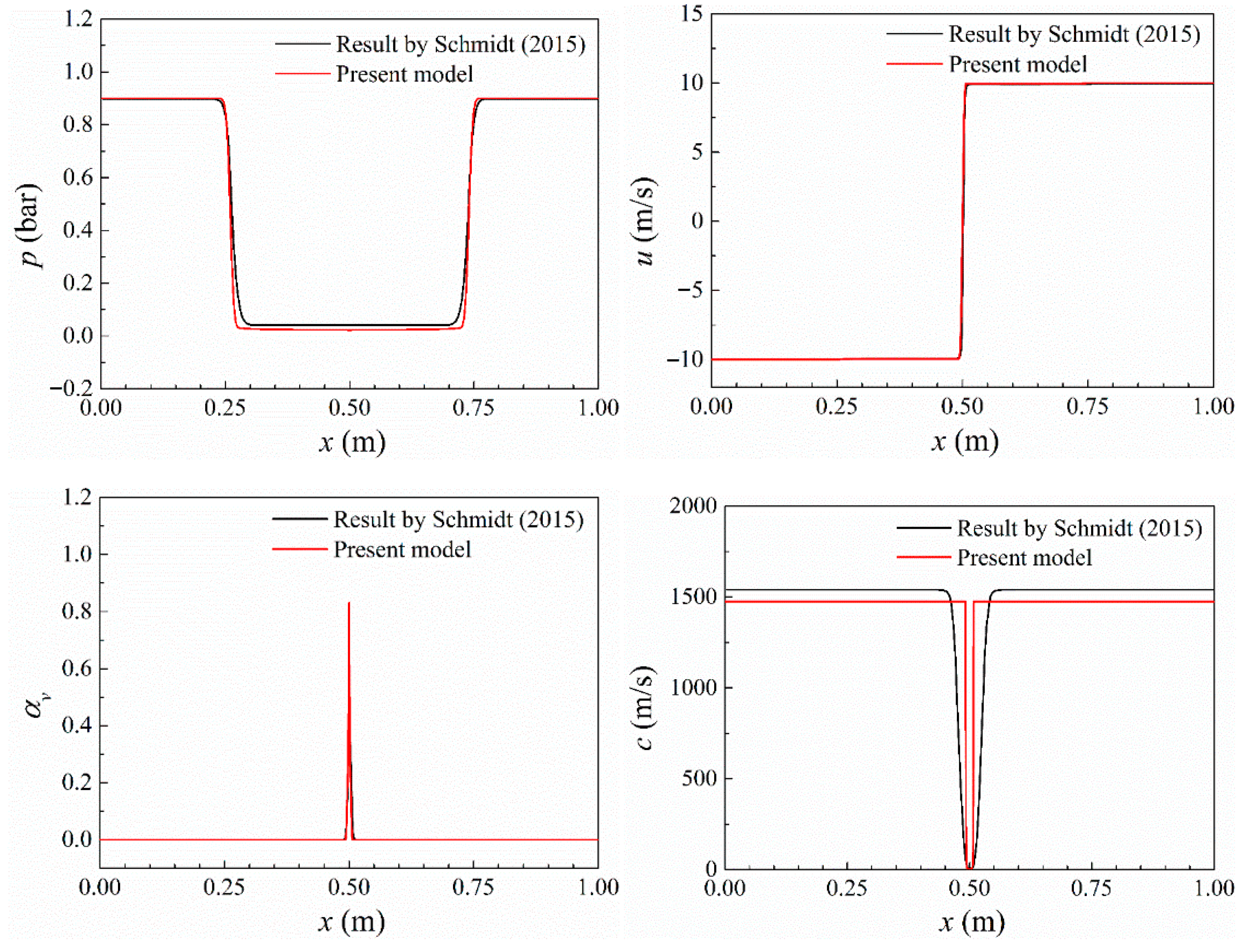
4.1. Case 1: 1-D Two-Phase Time-Dependent Test Case

In this section, the compressible cavitation model is used to describe the effects of a density reduction below the density value of the saturated liquid induced by two symmetrical expansion waves, as in the numerical setup defined by Schmidt [40]. The domain consists of a 1-D tube with a length of 1 m. At time $t$ = 0 s, the tube is full of pure liquid water, and the pressure is constant with a value of $p$= 0.9 bar. The velocity field is assumed to jump at $x$ = 0.5 m from the left velocity, $u_L$ = −10 m/s, to the right velocity, $u_R$= 10 m/s, to force the phase change from liquid to vapor to occur. Furthermore, the domain is divided into 1000 cells (four equally spaced cells in the $y$ direction and two-hundred-fifty in the $x$ direction), and the time integration is performed using the first-order implicit scheme with a time step $∆t$ = 1 × 10⁻⁷ s.

To verify the implementation of the compressible cavitation model, the current numerical results were compared with the ones obtained by Schmidt [40]. Figure 2 presents the pressure, the velocity, the vapor volume fraction, and the sound speed distributions along the tube at time $t$= 1.5 × 10⁻⁴ s using the present compressible cavitation model and the results obtained by Schmidt [40]. Without experiencing numerical oscillations in regions with high gradients, the currently implemented solver is proved to be numerically stable. Furthermore, the distribution of the flow quantities along the tube is almost identical between the current ones and those extracted from the reference simulation. The precise agreement between both sets of results demonstrates the validity of the implemented compressible cavitation model.

4.2. Case 2: Cavitating Flow over a Circular Cylinder

The present simulations of the non-cavitating and cavitating flows over a stationary cylinder were performed with a large 2D computational domain of dimensionless dimensions relative to the cylinder diameter, D, in the horizontal and vertical ranges −50 ≤ $x/D$ ≤ 50 and −50 ≤ $y/D$ ≤ 50, respectively, to avoid the effect of the domain boundaries, as depicted in Figure 3. The cylinder is located in position (0, 0), and the number of grid elements in the circumferential and radial directions are 480 and 220, respectively. The symbol $\theta$ represents the angle around the cylinder surface measured from its front stagnation point. The inflow condition of $u=u_{ref}$, and the pressure condition of $p=p_{ref}$ is set at the boundaries located at $x/D$ = −50 and $x/D$ = 50, respectively, while the symmetry condition is used at the top and bottom boundaries.

The drag and lift coefficients, denoted as $C_D$ and $C_L$, are defined as:

$$C_D={\displaystyle \frac{F_x}{\frac{1}{2}{\rho }_l{U_{ref}}^{2}D}}$$

(39)

$$C_L={\displaystyle \frac{F_y}{\frac{1}{2}{\rho }_l{ref}^{2}D}}$$

(40)

where $F_x$ and $F_y$ are the streamwise and transverse components of the force acting on the cylinder surface, respectively, and $U_{ref}$ is the free-stream velocity.

The unsteady vortex shedding case is calculated for liquid water at $Re$ = 200 as in previous studies [21,41,42,43,44,45,46,47]. Vortices are generated on the cylinder surface and detach alternatively from its upper and lower surfaces, which results in fluctuations of $C_D$ and $C_L$ as shown in Figure 4. The time average value of $C_D$, denoted as $C_{D,av}$, the maximum value of $C_L$, denoted as $C_{L,max}$, and the $St$ value are listed in

Table 1. Comparison of $C_{D,av}$, $C_{L,max}$, and $St$ values between the current simulation and the results previously published by other authors for a circular cylinder at $Re$ = 200 without cavitation.

	${\mathit{C}}_{\mathit{D},\mathit{a}\mathit{v}}$	${\mathit{C}}_{\mathit{L},\mathit{m}\mathit{a}\mathit{x}}$	$\mathit{S}\mathit{t}$
Braza et al. [41]	1.40	0.75	0.20
Ding et al. [42]	1.35	0.66	0.196
Seo et al. [43]	1.08	0.60	0.19
Harichandan and Roy [44]	1.32	0.60	0.194
Qu et al. [45]	1.32	0.66	0.196
Gnanaskandan et al. [21]	-	-	0.198
Kim and Choi [46]	1.35	0.70	0.197
Hong and Son [47]	1.32	0.66	0.194
Current simulation	1.32	0.65	0.194

and compared with published data obtained by different authors using different meshes and methods. It is confirmed that the present results match well with the reference values.

The simulations are extended to cavitation conditions at $\sigma$= 1.0. As shown in Figure 5, the oscillating flow around the cylinder results in $C_D$ and $C_L$ fluctuations. The corresponding $C_{D,av}$, $C_{L,max}$, and $St$ values are listed in

Table 2. Comparison of $C_{D,av}$ and $C_{L,max}$, and $St$ values between the current simulation and the results previously published by other authors for a circular cylinder at $Re$ = 200 at $\sigma$ = 1.0.

	${\mathit{C}}_{\mathit{D},\mathit{a}\mathit{v}}$	${\mathit{C}}_{\mathit{L},\mathit{m}\mathit{a}\mathit{x}}$	$\mathit{S}\mathit{t}$
Seo et al. [43]	1.08	0.42	0.16
Gnanaskandan and Mahesh [21]	1.10	0.56	0.16
Hong and Son [47]	-	-	0.177
Current simulation	1.22	0.30	0.17

and compared with previous results obtained by other authors. As the liquid pressure decreases to $p_v$, cavitation occurs around the lateral surface of the cylinder, and then the vaporous bubbles detach from the cylinder surface and travel within the shed vortices. The positive velocity divergence caused by the appearance of cavitation leads to vorticity dilatation, thus elongating and weakening the shed vortices [21]. Therefore, the computed shedding frequencies are reduced to $St$= 0.17, which is comparable to the corresponding prediction of 0.16 reported by Seo et al. [43] and Gnanaskandan and Mahesh [21], and of 0.177 reported by Hong and Son [47]. Moreover, Figure 6 compares the instantaneous vorticity contour colored with vapor volume fraction at $\sigma$ = 1.0 obtained by Gnanaskandan and Mahesh [21] and the present method and shows similar results.

5. Results

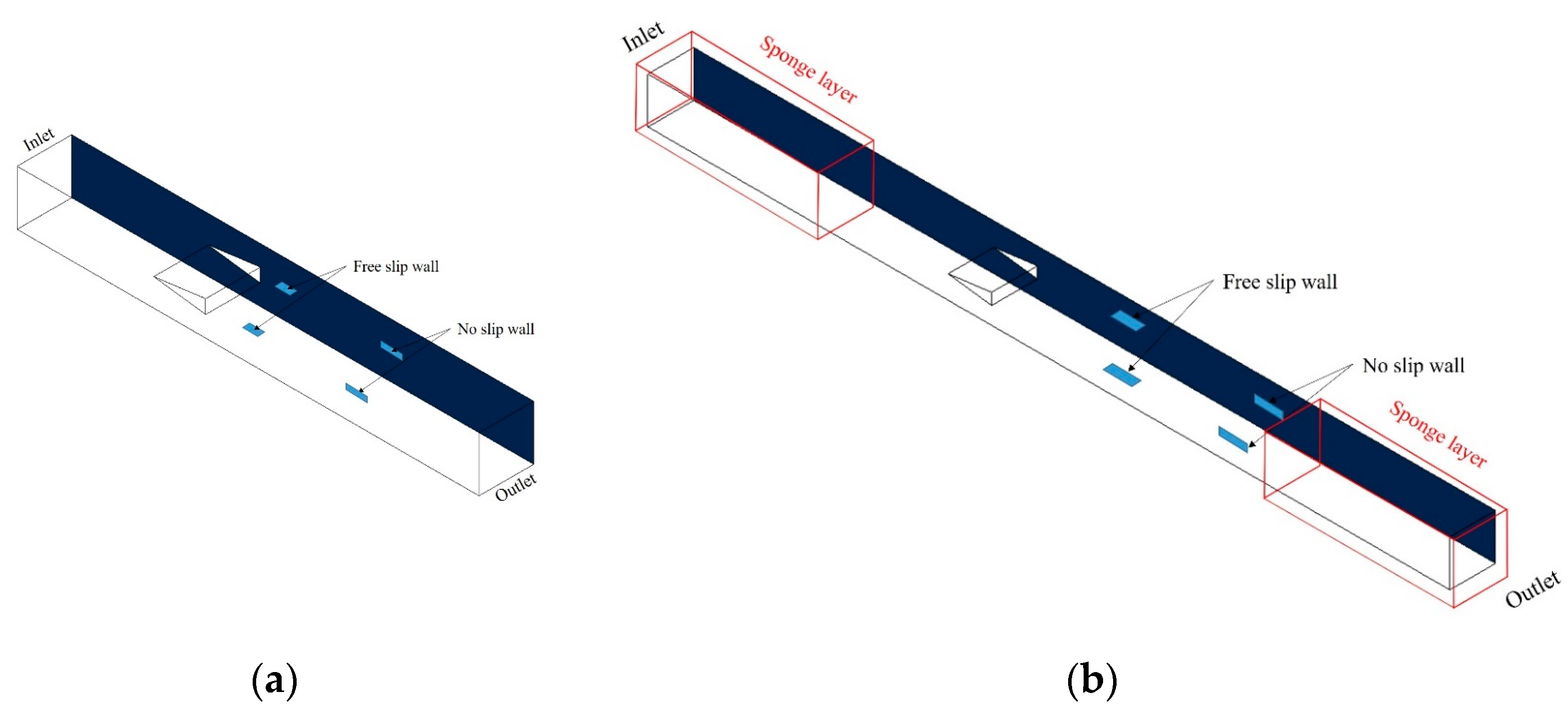
5.1. Computational Domain and Boundary Conditions

Figure 7 shows the dimensions of the computational domain to simulate the flow around a wedge, which are the same as the ones used in the experimental setup presented by Wu et al. [8]. The cross-section of the tunnel is rectangular, and its width is 4 D, where D is the height of the wedge base, which is equal to 0.019 m. The span of the wedge is 4 D. For the incompressible cavitation case, the inlet is located 13.5 D upstream from the wedge’s trailing edge plane, and the outlet is 19.5 D downstream from it. For the compressible cavitating simulation, the fluid domain is extended to implement the sponge layers at the inlet and outlet boundaries, which are located 25.9 D upstream and 36.6 D downstream of the trailing edge, respectively.

The flow around the wedge was simulated using the DDES model to capture the globally unstable flow characteristics. Such flow has the feature that the turbulence in the separated zone is independent of the turbulence within the incoming attached boundary layer [48]. This flow feature can require reducing significantly the mesh resolution. Following the suggestions provided by ANSYS Fluent [48], more than 20 cells per characteristic length, D, are sufficient to resolve the main flow instability. Furthermore, an isotropic cell (Δx = Δy = Δz) was used in the area near the trailing edge of the wedge to avoid the numerical error resulting from cells with too large aspect ratios. To assess the effects of mesh refinement on the calculations, three meshes with different refinements were tested, as listed in

Table 3. Characteristic parameters of the different meshes considered for the sensitivity test.

Name	Number of Cells	D/Δx
M1	1.39 × 106	20
M2	2.75 × 106	26
M3	4.13 × 106	30

. The topology of mesh M1 around the wedge is depicted in Figure 8a,b.

For the non-cavitating case, the inlet boundary condition was set as a uniform inflow velocity, $U_{ref}$ = 6 m/s, and the outlet type boundary condition was set as shown in Figure 9a. For the cavitation case at $\sigma$= 1.9, the corresponding total pressure was specified at the inlet boundary condition, and the fixed mass flowrate boundary condition was fixed at the outlet. To absorb the pressure wave generated by the compressible fluid and avoid reflections, sponge layer boundaries were added at the inlet and outlet areas [39], as depicted in Figure 9b. The specific values of the different boundary conditions for the two operating conditions without and with cavitation are detailed in

Table 4. Specific values of the boundary conditions for the non-cavitation and cavitation conditions.

σ	Inlet Boundary	Value	Outlet Boundary	Value	Top Wall	Bottom Wall	Other Walls
Non-cavitation	Fixed velocity	6 m/s	Outlet	-	FSW	FSW	NSW
1.9	Total pressure	54,540 Pa	Mass flowrate	34.66 kg/s	FSW	FSW	NSW

Free slip wall: FSW, No slip wall: NSW.

.

All the simulations were run with ANSYS Fluent using the bounded central difference (BCD) advected scheme and a time step of 5 × 10⁻⁵ s, where the corresponding advected Courant number is less than one behind the wedge.

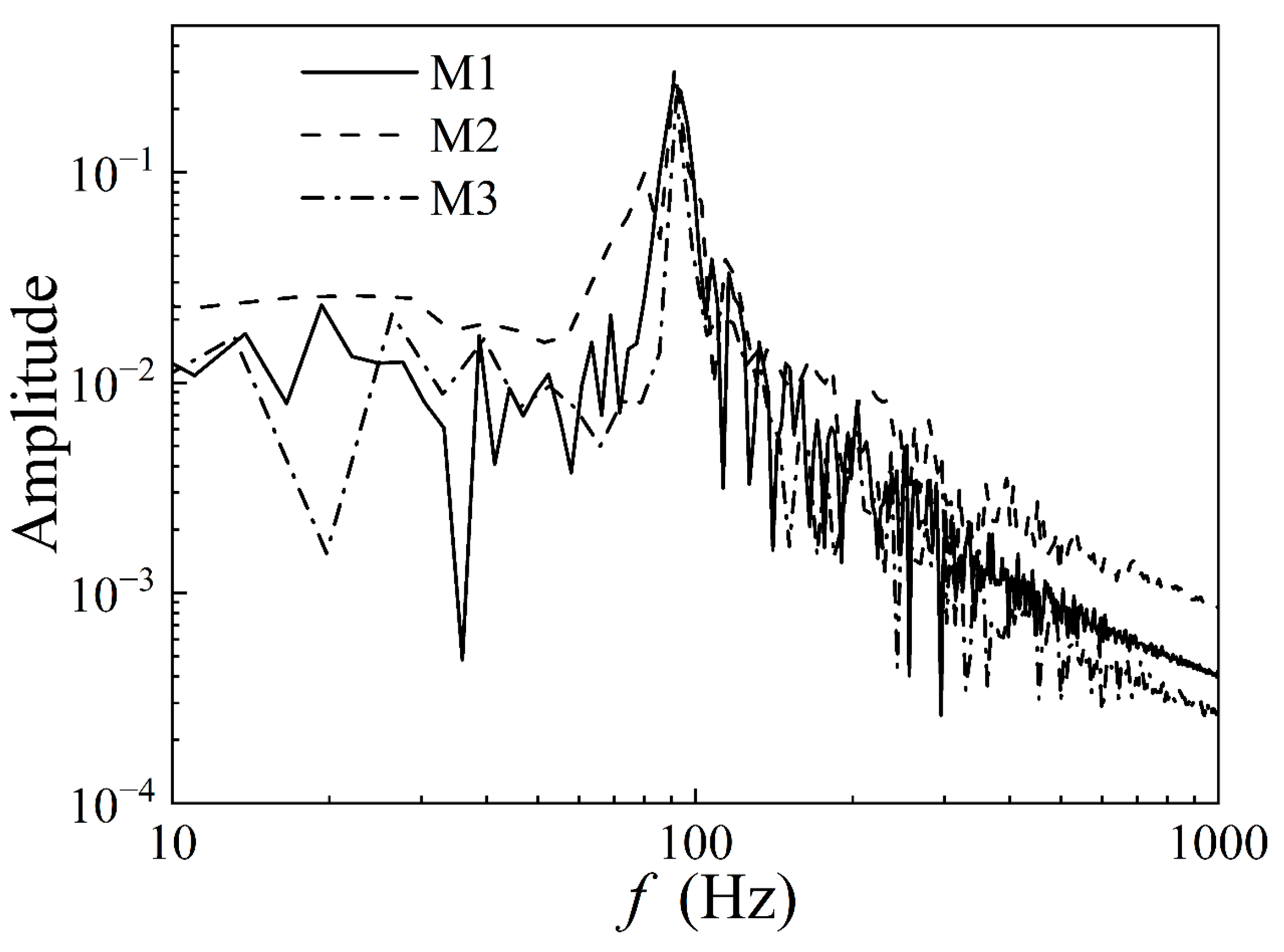
5.2. Verification and Validation of the Non-Cavitating Case

Figure 10 shows the spectra of the simulated lift coefficient calculated using FFT for the three different grid refinements at non-cavitation conditions with the compressible model. It can be seen that for all the meshes the same maximum frequency peak is obtained with similar amplitudes even when the coarse mesh is used. Therefore, to save computational resources, the mesh M1 has been selected and used for the following analysis.

As presented in Figure 10, the main frequency peak corresponding to the vortex shedding frequency is found around 91 Hz, where y is in good agreement with the value of 90 Hz obtained by Wu et al. [8].

The numerically obtained $C_p$ on the surface of the wedge is plotted in Figure 11. Here, the position at $y=\pm 0.5$ D corresponds to the two vertices at the truncated trailing edge. It can be seen that, at the center line of the base of the wedge, the value of $C_p$ = −1.5 is exactly the same as the experimental value reported by Wu et al. [8]. Therefore, it can be concluded that, in the non-cavitating case, the current numerical solution of the unsteady flow field provides a reasonable resemblance to the flow conditions measured during the experiment carried out by Wu et al. [8].

5.3. Assessment of the Compressible Cavitation Model

Using the validated incompressible and compressible modeling approaches presented in the previous sections, the cavitating wake behind the wedge at $U_{ref}$= 6 m/s and $\sigma$= 1.9 was calculated numerically to demonstrate the effects of fluid compressibility on the dynamics of the cavitating vortex shedding behind the wedge.

5.3.1. Pressure on the Wedge Surface

Figure 12 compares the mean values of $C_p$ on the wedge surface using both the incompressible and the compressible cavitation solvers, and it can be seen that the results are exactly the same. Moreover, the numerical $C_p$ of −1.4 at the centerline of the base of the wedge is in good agreement with the experimental value of −1.45 obtained by Wu et al. [8].

5.3.2. Unsteady Loads on the Wedge Surface

For comparison, Figure 13 shows the time histories of $C_L$ and their spectra with the incompressible and compressible cavitation solvers at $\sigma$= 1.9. It can be seen that both solvers predict the same value of 210 Hz for the vortex shedding frequency behind the wedge. Such a result is in good agreement with the dominant frequency reported by Wu et al. As shown in Figure 13b, the shape and amplitudes of the spectra obtained with the incompressible and compressible cavitation solvers are quite similar for the lower frequencies below 800 Hz. However, at high frequencies above 1000 Hz, the spectra obtained with the incompressible cavitation solver present lower amplitude values than with the compressible cavitation solver. It is interesting to note that similar results were observed in the investigation of cloud cavitation around the hydrofoil conducted by Wang et al. [22].

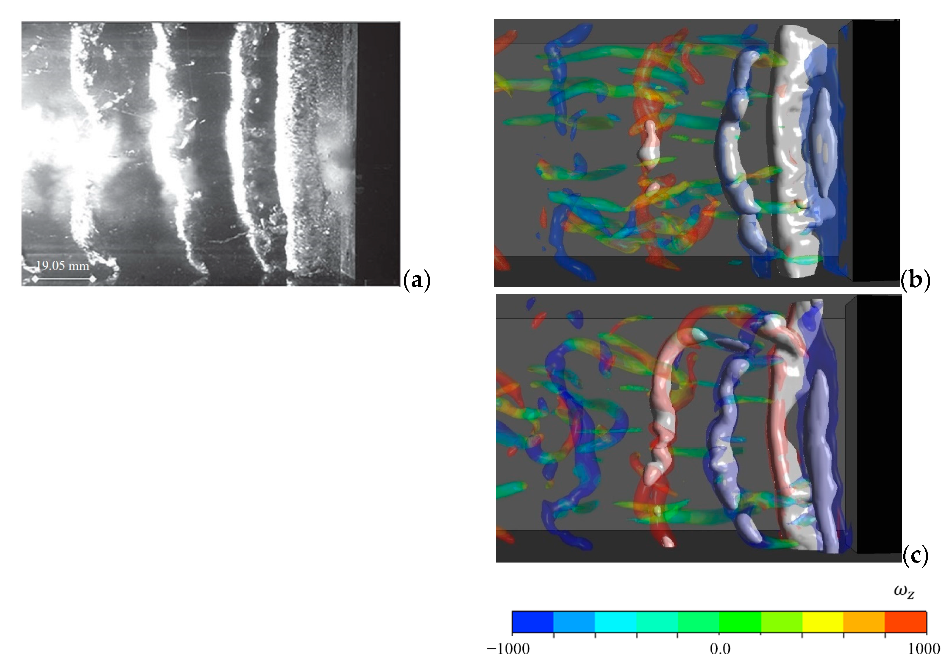
5.3.3. Cavitation Structures

Figure 14 shows a visualization of the 3D cavitation structures inside the shed vortices using iso-surface plots, with the numerical results obtained with both the incompressible and the compressible cavitation solvers. They are compared in the same figure with the photographs taken during the experimental tests carried out by Wu et al. [8]. It can be seen that the first few pairs of spanwise vortex cores (identified with the $Q$ criterion) are filled with vapor, and these cavity structures (represented with iso-surfaces of ${\alpha }_v$ = 0.05) are advected downstream. Furthermore, the relative positions of the vortices and the spacings obtained with the incompressible and compressible cavitation models are quite similar, and they align well with the experimental results.

Figure 15 shows the simulated instantaneous field of ${\alpha }_v$ in the cavitating wake at different instants of time obtained with the incompressible (Incomp.) and compressible (Comp.) cavitation solvers at $\sigma$ = 1.9 as well as the experimental (Exp.) images reported by Wu et al. [8] using time-resolved X-ray densitometry. All of them show clearly the periodically shed vortices at the vortex shedding frequency. The evolution of the cavitation structures with time confirms that the periodic shedding is governed by the alternating shedding vortex street behind the wedge. In each shedding period, a cavity starts to form and fill the center of the shed vortex. Then, the cavitating vortex is advected from the attached boundary layer and shed from the trailing edge. The alternating cavitating shedding vortices form the vortex street behind the wedge. The comparison between numerical results using incompressible and compressible cavitation solvers and the experimental results indicates that both cavitation solvers can capture the main flow characteristics in terms of the cavities morphology and their relative position, as can be seen in Figure 15a,c.

Figure 16 shows the time average void fraction field calculated with the incompressible (Incomp.) and compressible (Comp.) cavitation solvers and the experimental results. It can be seen that the simulations with two different cavitation solvers produce almost indistinguishable mean and RMS void fraction fields behind the wedge. The shape of mean cavity structures obtained numerically is comparable to the pattern observed in the experimental image. Note that there is a downstream offset in the mean and RMS void fraction fields between the numerical and the experimental results, which may be due to the low numerical resolution of the locally unstable flow structures within the detachment area.

6. Conclusions

In this study, the numerical results obtained with both incompressible and compressible cavitation solvers were compared to assess the effects of fluid compressibility on the characteristics and dynamics of the cavitating flow behind a wedge. In relation to the experimental results obtained by Wu et al. [5], it was found:

• Both cavitation solvers provide similar results to the experimental ones in terms of mean pressure and hydrodynamic forces.
• Both cavitation solvers provide almost identical results of the dominant vortex shedding frequency and the instantaneous and mean void fraction fields.
• The spectral content of the simulated hydrodynamic forces is similar with both solvers for low frequencies, but, for higher frequencies, the amplitudes are larger and the content is better resolved with the compressible solver.

In conclusion, it was found that the compressibility effects on the cavitating vortex shedding behind the wedge can be simulated with the compressible solver and that they induce high-frequency phenomena, although the average quantities are not significantly affected in comparison with the incompressible solver results.

References

1. Arndt, R.E.A. Cavitation in Fluid Machinery and Hydraulic Structures. Annu. Rev. Fluid Mech. 1981, 13, 273–326. [Google Scholar] [CrossRef]
2. Escaler, X.; Egusquiza, E.; Farhat, M.; Avellan, F.; Coussirat, M. Detection of Cavitation in Hydraulic Turbines. Mech. Syst. Signal Process. 2006, 20, 983–1007. [Google Scholar] [CrossRef]
3. Gu, Y.; Sun, H.; Wang, C.; Lu, R.; Liu, B.; Ge, J. Effect of Trimmed Rear Shroud on Performance and Axial Thrust of Multi-Stage Centrifugal Pump with Emphasis on Visualizing Flow Losses. J. Fluids Eng. 2024, 146, 011204. [Google Scholar] [CrossRef]
4. Franc, J.P.; Michel, J.M. Fundamentals of Cavitation; Springer Science & Business Media: Berlin/Heidelberg, Germany, 2006. [Google Scholar]
5. Young, J.O.; Holl, J.W. Effects of Cavitation on Periodic Wakes behind Symmetric Wedges. J. Basic Eng. 1966, 88, 163–176. [Google Scholar] [CrossRef]
6. Belahadji, B.; Franc, J.P.; Michel, J.M. Cavitation in the Rotational Structures of a Turbulent Wake. J. Fluid Mech. 1995, 287, 383–403. [Google Scholar] [CrossRef]
7. Ausoni, P.; Farhat, M.; Escaler, X.; Egusquiza, E.; Avellan, F. Cavitation Influence on von Kármán Vortex Shedding and Induced Hydrofoil Vibrations. J. Fluids Eng. 2007, 129, 966–973. [Google Scholar] [CrossRef]
8. Wu, J.; Deijlen, L.; Bhatt, A.; Ganesh, H.; Ceccio, S.L. Cavitation Dynamics and Vortex Shedding in the Wake of a Bluff Body. J. Fluid Mech. 2021, 917, A26. [Google Scholar] [CrossRef]
9. Niedźwiedzka, A.; Schnerr, G.H.; Sobieski, W. Review of Numerical Models of Cavitating Flows with the Use of the Homogeneous Approach. Arch. Thermodyn. 2016, 37, 71–88. [Google Scholar] [CrossRef]
10. Folden, T.S.; Aschmoneit, F.J. A Classification and Review of Cavitation Models with an Emphasis on Physical Aspects of Cavitation. Phys. Fluids 2023, 35, 081301. [Google Scholar] [CrossRef]
11. Coutier-Delgosha, O.; Reboud, J.L.; Delannoy, Y. Numerical Simulation of the Unsteady Behaviour of Cavitating Flows. Int. J. Numer. Methods Fluids 2003, 42, 527–548. [Google Scholar] [CrossRef]
12. Ji, B.; Luo, X.; Arndt, R.E.A.; Wu, Y. Numerical Simulation of Three Dimensional Cavitation Shedding Dynamics with Special Emphasis on Cavitation–Vortex Interaction. Ocean Eng. 2014, 87, 64–77. [Google Scholar] [CrossRef]
13. Gnanaskandan, A.; Mahesh, K. Large Eddy Simulation of the Transition from Sheet to Cloud Cavitation over a Wedge. Int. J. Multiph. Flow 2016, 83, 86–102. [Google Scholar] [CrossRef]
14. Callenaere, M.; Franc, J.P.; Michel, J.M.; Riondet, M. The Cavitation Instability Induced by the Development of a Re-Entrant Jet. J. Fluid Mech. 2001, 444, 223–256. [Google Scholar] [CrossRef]
15. Kawanami, Y.; Kato, H.; Yamaguchi, H.; Tanimura, M.; Tagaya, Y. Mechanism and Control of Cloud Cavitation. J. Fluids Eng. 1997, 119, 778–794. [Google Scholar] [CrossRef]
16. Laberteaux, K.R.; Ceccio, S.L. Partial Cavity Flows. Part 1. Cavities Forming on Models without Spanwise Variation. J. Fluid Mech. 2001, 431, 1–41. [Google Scholar] [CrossRef]
17. Leroux, J.-B.; Astolfi, J.A.; Billard, J.Y. An Experimental Study of Unsteady Partial Cavitation. J. Fluids Eng. 2004, 126, 94–101. [Google Scholar] [CrossRef]
18. Wu, J.; Ganesh, H.; Ceccio, S. Multimodal Partial Cavity Shedding on a Two-Dimensional Hydrofoil and Its Relation to the Presence of Bubbly Shocks. Exp. Fluids 2019, 60, 66. [Google Scholar] [CrossRef]
19. Ganesh, H.; Mäkiharju, S.A.; Ceccio, S.L. Bubbly Shock Propagation as a Mechanism for Sheet-to-Cloud Transition of Partial Cavities. J. Fluid Mech. 2016, 802, 37–78. [Google Scholar] [CrossRef]
20. Bhatt, A.; Ganesh, H.; Ceccio, S.L. Partial Cavity Shedding on a Hydrofoil Resulting from Re-Entrant Flow and Bubbly Shock Waves. J. Fluid Mech. 2023, 957, A28. [Google Scholar] [CrossRef]
21. Gnanaskandan, A.; Mahesh, K. Numerical Investigation of Near-Wake Characteristics of Cavitating Flow over a Circular Cylinder. J. Fluid Mech. 2016, 790, 453–491. [Google Scholar] [CrossRef]
22. Wang, C.; Wang, G.; Huang, B. Characteristics and Dynamics of Compressible Cavitating Flows with Special Emphasis on Compressibility Effects. Int. J. Multiph. Flow 2020, 130, 103357. [Google Scholar] [CrossRef]
23. Vaca-Revelo, D.; Gnanaskandan, A. Numerical Assessment of the Condensation Shock Mechanism in Sheet to Cloud Cavitation Transition. Int. J. Multiph. Flow 2023, 169, 104616. [Google Scholar] [CrossRef]
24. Katz, J. Cavitation Phenomena within Regions of Flow Separation. J. Fluid Mech. 1984, 140, 397–436. [Google Scholar] [CrossRef]
25. O’Hern, T.J. An Experimental Investigation of Turbulent Shear Flow Cavitation. J. Fluid Mech. 1990, 215, 365–391. [Google Scholar] [CrossRef]
26. Iyer, C.O.; Ceccio, S.L. The Influence of Developed Cavitation on the Flow of a Turbulent Shear Layer. Phys. Fluids 2002, 14, 3414–3431. [Google Scholar] [CrossRef]
27. Choi, J.; Ceccio, S.L. Dynamics and Noise Emission of Vortex Cavitation Bubbles. J. Fluid Mech. 2007, 575, 1–26. [Google Scholar] [CrossRef]
28. Agarwal, K.; Ram, O.; Lu, Y.; Katz, J. On the Pressure Field, Nuclei Dynamics and Their Relation to Cavitation Inception in a Turbulent Shear Layer. J. Fluid Mech. 2023, 966, A31. [Google Scholar] [CrossRef]
29. Wang, Z.; Cheng, H.; Ji, B. Euler–Lagrange Study of Cavitating Turbulent Flow around a Hydrofoil. Phys. Fluids 2021, 33, 112108. [Google Scholar] [CrossRef]
30. Wang, Z.; Cheng, H.; Ji, B.; Peng, X. Numerical Investigation of Inner Structure and Its Formation Mechanism of Cloud Cavitating Flow. Int. J. Multiph. Flow 2023, 165, 104484. [Google Scholar] [CrossRef]
31. Brandao, F.L.; Bhatt, M.; Mahesh, K. Numerical Study of Cavitation Regimes in Flow over a Circular Cylinder. J. Fluid Mech. 2020, 885, A19. [Google Scholar] [CrossRef]
32. Park, S.; Seok, W.; Park, S.T.; Rhee, S.H.; Choe, Y.; Kim, C.; Kim, J.H.; Ahn, B.K. Compressibility Effects on Cavity Dynamics behind a Two-Dimensional Wedge. J. Mar. Sci. Eng. 2020, 8, 39. [Google Scholar] [CrossRef]
33. Wang, Z.; Cheng, H.; Bensow, R.E.; Ji, B. Numerical Evaluation of the Bubble Dynamic Influence on the Characteristics of Multiscale Cavitating Flow in the Bluff Body Wake. Int. J. Multiph. Flow 2024, 175, 104818. [Google Scholar] [CrossRef]
34. Zwart, P.; Gerber, A.G.; Belamri, T. A Two-Phase Flow Model for Predicting Cavitation Dynamics. In Proceedings of the Fifth International Conference on Multiphase Flow, Yokohama, Japan, 30 May–4 June 2004. [Google Scholar]
35. Egerer, C.P.; Schmidt, S.J.; Hickel, S.; Adams, N.A. Efficient Implicit LES Method for the Simulation of Turbulent Cavitating Flows. J. Comput. Phys. 2016, 316, 453–469. [Google Scholar] [CrossRef]
36. Tong, S.-Y.; Zhang, S.; Wang, S.-P.; Li, S. Characteristics of the Bubble-Induced Pressure, Force, and Impulse on a Rigid Wall. Ocean Eng. 2022, 255, 111484. [Google Scholar] [CrossRef]
37. Li, H.; Vasquez, S.A. Numerical Simulation of Steady and Unsteady Compressible Multiphase Flows. In Proceedings of the ASME 2012 International Mechanical Engineering Congress and Exposition, Houston, TX, USA, 9–15 November 2012; pp. 2239–2251. [Google Scholar]
38. Brunhart, M.; Soteriou, C.; Gavaises, M.; Karathanassis, I.; Koukouvinis, P.; Jahangir, S.; Poelma, C. Investigation of Cavitation and Vapor Shedding Mechanisms in a Venturi Nozzle. Phys. Fluids 2020, 32, 083306. [Google Scholar] [CrossRef]
39. Mani, A. Analysis and Optimization of Numerical Sponge Layers as a Nonreflective Boundary Treatment. J. Comput. Phys. 2012, 231, 704–716. [Google Scholar] [CrossRef]
40. Schmidt, S.J. A Low Mach Number Consistent Compressible Approach for Simulation of Cavitating Flows. Ph.D. Thesis, Technical University of Munich, Munich, Germany, 2015. [Google Scholar]
41. Braza, M.; Chassaing, P.; Minh, H.H. Numerical Study and Physical Analysis of the Pressure and Velocity Fields in the near Wake of a Circular Cylinder. J. Fluid Mech. 1986, 165, 79–130. [Google Scholar] [CrossRef]
42. Ding, H.; Shu, C.; Yeo, K.S.; Xu, D. Numerical Simulation of Flows around Two Circular Cylinders by Mesh-Free Least Square-Based Finite Difference Methods. Int. J. Numer. Methods Fluids 2007, 53, 305–332. [Google Scholar] [CrossRef]
43. Seo, J.H.; Moon, Y.J.; Shin, B.R. Prediction of Cavitating Flow Noise by Direct Numerical Simulation. J. Comput. Phys. 2008, 227, 6511–6531. [Google Scholar] [CrossRef]
44. Harichandan, A.B.; Roy, A. Numerical Investigation of Flow Past Single and Tandem Cylindrical Bodies in the Vicinity of a Plane Wall. J. Fluids Struct. 2012, 33, 19–43. [Google Scholar] [CrossRef]
45. Qu, L.; Norberg, C.; Davidson, L.; Peng, S.-H.; Wang, F. Quantitative Numerical Analysis of Flow Past a Circular Cylinder at Reynolds Number between 50 and 200. J. Fluids Struct. 2013, 39, 347–370. [Google Scholar] [CrossRef]
46. Kim, K.H.; Choi, J.I. Lock-in Regions of Laminar Flows over a Streamwise Oscillating Circular Cylinder. J. Fluid Mech. 2019, 858, 315–351. [Google Scholar] [CrossRef]
47. Hong, S.; Son, G. Numerical Simulation of Cavitating Flows around an Oscillating Circular Cylinder. Ocean Eng. 2021, 226, 108739. [Google Scholar] [CrossRef]
48. Menter, F.R. Best Practice: Scale-Resolving Simulations in ANSYS CFD; ANSYS Germany GmbH: Darmstadt, Germany, 2015. [Google Scholar]
Figure 1. Schematic of the sponge layer implementation.
Fluids 09 00218 g001
Figure 2. Comparison of flow quantities obtained with the present model and the simulation by Schmidt (2015) [40] at time t   = 1.5 × 10⁻⁴ s for the 1-D two-phase time-dependent case.
Fluids 09 00218 g002
Figure 3. Details of the computational meshes around the circular cylinder: (a) whole domain and (b) region near the circular cylinder.
Fluids 09 00218 g003
Figure 4. Time history of C D and C L for the non-cavitation regime.
Fluids 09 00218 g004
Figure 5. Time history of C D and C L for the cavitation regime at σ   = 1.0.
Fluids 09 00218 g005
Figure 6. Comparison of the instantaneous vorticity contour colored with vapor volume fraction at σ = 1.0 between (a) Gnanaskandan and Mahesh [21] and (b) the current results.
Fluids 09 00218 g006
Figure 7. Computational domain for (a) the incompressible and (b) the compressible cavitation models.
Fluids 09 00218 g007
Figure 8. Views of the mesh topology around the wedge from (a) the side and (b) the top.
Fluids 09 00218 g008
Figure 9. Fluid domain and boundary conditions defined to simulate the cavitating flow behind the wedge using an (a) incompressible cavitation model and a (b) compressible cavitation model.
Fluids 09 00218 g009
Figure 10. Spectra of the lift coefficient for three different mesh refinements in the case of non-cavitation.
Fluids 09 00218 g010
Figure 11. Simulated versus measured C p values around the surface of the wedge in the non-cavitating condition [8].
Fluids 09 00218 g011
Figure 12. Simulated versus measured C p values around the surface of the wedge using the incompressible and compressible cavitation models in the cavitation condition, with σ = 1.9 [8].
Fluids 09 00218 g012
Figure 13. (a) Lift coefficient time histories and (b) corresponding spectra with the incompressible and the compressible cavitation models at σ   = 1.9.
Fluids 09 00218 g013
Figure 14. Comparisons of (a) the experimentally [8] and the numerically obtained cavity structures using (b) the incompressible and (c) the compressible cavitation models at σ   = 1.9. The vortical structures are identified with an iso-surface of α v   = 0.05, and the vorticity level is indicated with the Q criterion.
Fluids 09 00218 g014
Figure 15. Comparisons of the experimentally (Exp.) [8] and numerically obtained void fraction contour plots at different instants of time during the vortex shedding using the incompressible (Incomp.) and the compressible (Comp.) cavitation models at σ   = 1.9.
Fluids 09 00218 g015aFluids 09 00218 g015b
Figure 16. Comparisons of the experimentally (Exp.) [8] and numerically obtained time average (a) and (b) RMS void fraction fields using the incompressible (Incomp.) and the compressible (Comp.) cavitation models at σ   = 1.9.
Fluids 09 00218 g016