Coulomb Driven Electro-Convection within Two Stacked Layers of Miscible Dielectric Liquids ^†

Abstract

This article investigates the behavior of two parallel layers of different miscible dielectric liquids enclosed and sandwiched between two electrodes. By applying an electric potential to one electrode while grounding the other, electro-convection occurs when the electric Rayleigh number exceeds a critical value, setting the fluid into motion and resulting in rapid mixing between the two liquids. A numerical model is developed to account for the varying ionic mobility and permittivity of the two liquids, considering their evolution based on the relative concentration field. The simulations confirm that electro-convection significantly enhances the mixing between the two liquids, as expected. Additionally, intriguing ripples are observed near the initial interface during the early stages of electro-convection instability growth. To explain and describe the flow dynamics in terms of stability analysis, a semi-analytical model is presented. This study provides insights into the mixing behavior and flow dynamics of miscible dielectric liquids under the influence of electro-convection. The findings contribute to a better understanding of the underlying mechanisms and can be valuable for applications such as microfluidics, energy conversion, and mixing processes. Further research is encouraged to explore additional parameters and optimize the control of electro-convection for practical applications.

1. Introduction

Electrohydrodynamics (EHD) is an interdisciplinary field that explores the interaction between fluid flow and electric fields [1]. EHD techniques offer significant potential in various applications, including flow control, heat and mass transfer enhancement, and micro-electromechanical systems (MEMS) [2].

In this study, two parallel layers of two dielectric liquids are stacked into an enclosed cavity. The two liquids are considered miscible, so that, even without any mechanical action, they tend to mix by molecular diffusion. However, this molecular diffusion may take a long time (depending on the diffusion coefficient between the two fluids) before reaching a homogeneous mixture. That is the reason why, in many industrial processes which deal with fluid mixing, one often uses mechanical devices based on rotative blades to increase the mixing. But this mechanical device has an extra energy cost. Another option could be to use the Coulomb force between two metallic electrodes that sandwiches the two layers to induce electro-convection to mix the two liquids.

When certain conditions are met, electric forces act on the layers of dielectric liquids, leading to electro-convection. Similar to how electro-convection enhances heat transfer [3,4,5], this effect can also be utilized to improve the mixing of two layers of dielectric liquids in contact.

In this context, it becomes crucial to determine the optimal electrical conditions, particularly the applied electric potential, to achieve the perfect mixing of the two specific dielectric liquids defined by their diffusion coefficient. A related experiment was conducted by the authors in [6,7], which closely relates to the work presented here. In this study, both liquids are characterized by different electric permittivity and ionic mobility. The objective is to gain a fundamental understanding of how the different properties of the liquids, their density, permittivity and ionic mobility influence the electro-soluto-convection phenomenon. Through this investigation, we aim to enhance our understanding of mass transfer efficiency and mixing enhancement between two miscible liquids with distinct properties.

The remainder of this paper is organized as follows:

In the next section, the physical and numerical models of two layers of miscible dielectric liquids subjected to an electric field applied between two horizontal parallel electrodes are detailed. Numerical results are presented and discussed in Section 3. Section 4 is devoted to the description of a semi-analytical model that confirms the trends observed in the numerical results. Finally, a conclusion is drawn up in Section 5.

2. Theoretical and Numerical Models

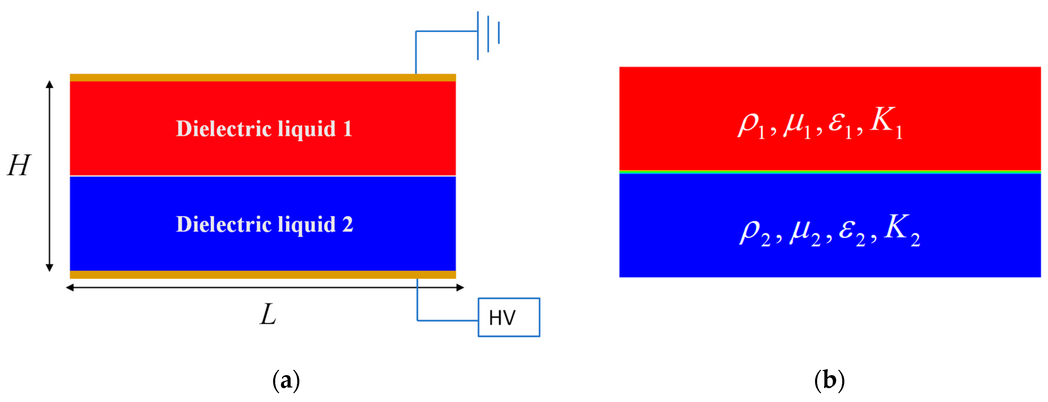
2.1. Problem Formuation

In this study, we investigate the behavior of two distinct layers of miscible dielectric liquid layers with equal thicknesses. These layers are positioned between two horizontal flat plate electrodes along the entire length of cavity, as depicted in Figure 1. One key aspect of this study is that these two liquids are Newtonian, incompressible, miscible, and perfectly insulating.

The two dielectric liquids considered in this study have different physical properties, different density ${\rho }_1 \mathrm{and} {\rho }_2$, different dynamic viscosity ${\mu }_1 \mathrm{and} {\mu }_2$, different permittivity ${\epsilon }_1 \mathrm{and} {\epsilon }_2$ as well as different ionic mobility $K_1 \mathrm{and} K_2$.

The main point is also that the two liquids are assumed to be miscible. This miscibility allows for the mixing to occur through molecular coefficient diffusion D.

When a sufficiently strong DC electric potential is applied across the two electrodes, charge injection takes place, leading to the generation of Coulomb electric body force. Under some circumstances, this force sets the liquids in motion by electro-convection, initiating the mixing process. This mechanical motion acts like an electric mixer and will significantly increase the degree of mixing between the two liquids, compared with a situation where molecular diffusion alone was likely to act.

The charge injection is assumed to be homogeneous and autonomous, which means the density of injected charges at the emitter electrode remains constant and unaffected by the local electric field and flow motion [8].

As it has been stated in many publications [8,9,10,11] the development of a subcritical bifurcation occurs as soon as the electric Rayleigh number T is above a critical one T_c. This subcritical bifurcation results from a strong nonlinear coupling between the electric field and the fluid velocity field. Even with extremely simple geometry configurations, this strong nonlinear interaction between the electric field (Maxwell’s equations) and the velocity field (Navier–Stokes equations) precludes the possibility of using analytical methods to determine the charge density distribution as well as all the dynamics of the flow.

In this study, we are going to numerically solve this coupled problem and analyze the enhanced mass transfer phenomena in a binary fluid due to unipolar charge injection.

2.2. Governing Equations

The governing equations include the mass conservation equation, the Navier–Stokes equations, the mass transfer equation, a reduced set of Maxwell’s equations, and some equations of state. Some basic assumptions need to be made, namely, (i) there is only one kind of ion in the liquid (unipolar injection); (ii) magnetic effect is negligible; (iii) fluids are perfect insulators; (iv) fluids are isothermal; and (v) the Boussinesq approximation for density is retained. The concept of the Boussinesq approximation, often related to the dependency of density on temperature, is also applied to the dependency of density on concentration. This approximation assumes that all physical properties of the fluid are considered constant, except for the density in the buoyancy term. In the buoyancy term, the fluid density is treated as a linear function of concentration C, and can be expressed as

$\rho ={\rho }_0\left(1-{\beta }_S(C-C_0)\right)$, where ${\rho }_0$ is the reference density of fluid 1 at concentration $C_0$ and ${\beta }_S$ is the volumetric expansion coefficient due to the concentration of fluid 1 [12].

The complete mathematical model leading to this coupled set of equations can be found in references [3,11,13].

$$\nabla ·\overrightarrow{u}=0$$

(1)

$${\displaystyle \frac{\partial (\rho \overrightarrow{u})}{\partial t}}+\nabla ·(\rho \overrightarrow{u}\overrightarrow{u}) = -\nabla p+\nabla ·\left(\mu \left(\overline{\overline{\nabla \overrightarrow{u}}}+{\overline{\overline{\nabla \overrightarrow{u}}}}^T\right)\right)+q\overrightarrow{E}-\left[{\displaystyle \frac{E^2}{2}}\nabla \epsilon \right]+\rho \overrightarrow{g}$$

(2)

$${\displaystyle \frac{\partial C}{\partial t}}+\overrightarrow{u} ·\nabla C=D{\nabla }^{2}C$$

(3)

$${\displaystyle \frac{\partial q}{\partial t}}+\nabla ·\left(\left(\overrightarrow{u}+K\overrightarrow{E}\right)q\right) = 0$$

(4)

$$\nabla ·\left(\epsilon \nabla V\right)=-q$$

(5)

$$\overrightarrow{E}=-\nabla V$$

(6)

$$\rho ={\rho }_0\left(1-{\beta }_S(C-C_0)\right)$$

(7)

$$\mu =C{\mu }_1+(1-C){\mu }_2$$

(8)

$$\epsilon =C{\epsilon }_1+(1-C){\epsilon }_2$$

(9)

$$K=C{K}_1+(1-C)K_2$$

(10)

Here, $\overrightarrow{u}$ and p stand for the velocity and the pressure field, respectively. C is the concentration field and D is the molecular diffusion between the two liquids.

$\rho , \mu ,\epsilon \mathrm{and} K$ are, respectively, the density, the dynamic viscosity, the permittivity and the ionic mobility of the mix. These quantities are related to the density, the dynamic viscosity, the permittivity, and the ionic mobility of each liquid ${\rho }_i, {\mu }_i,{\epsilon }_i, K_i$ and concentration C.

q stands for charge density, V stands for electric potential, and $\overrightarrow{E}$ is the electric field.

Fluid 1 is taken as the reference fluid to compute the concentration C.

For the sake of simplicity, the governing equations are non-dimensionalized based on the following scales:

H for length, $\Delta V$ for electric potential, $\Delta V/H$ for electric field, ${\mu }_{ref}/{\rho }_{ref}H$ for velocity, ${\rho }_{ref}{\left({\mu }_{ref}/{\rho }_{ref}H\right)}^2$ for pressure, and q₀ for the charge density. Under these assumptions, the dimensionless governing equations read now as

$$\nabla ·\overrightarrow{u}=0$$

(11)

$${\displaystyle \frac{\partial (\overrightarrow{u})}{\partial t}}+\nabla ·(\overrightarrow{u}\overrightarrow{u})=-\nabla p+\nabla ·\left(\mu \left(\overline{\overline{\nabla \overrightarrow{u}}}+{\overline{\overline{\nabla \overrightarrow{u}}}}^T\right)\right)+{\displaystyle \frac{C_{inj}{T}^2}{M^2}}q\overrightarrow{E}-{\displaystyle \frac{T^2}{M^2}}\left[{\displaystyle \frac{E^2}{2}}\nabla \epsilon \right]+{\displaystyle \frac{R{a}_s}{Sc}}C\overrightarrow{y}$$

(12)

$${\displaystyle \frac{\partial C}{\partial t}}+\overrightarrow{u} ·\nabla C={\displaystyle \frac{1}{Sc}}{\nabla }^{2}C$$

(13)

$${\displaystyle \frac{\partial q}{\partial t}}+\nabla ·\left(\left(\overrightarrow{u}+{\displaystyle \frac{T}{M^2}}K\overrightarrow{E}\right)q\right)=0$$

(14)

$$\nabla ·\left(\epsilon \nabla V\right)=-C_{inj}q$$

(15)

$$\overrightarrow{E}=-\nabla V$$

(16)

$$\rho =1-{\beta }_{S}C$$

(17)

$$\mu =C+(1-C){\mu }_{ratio}$$

(18)

$$\epsilon =C+(1-C){\epsilon }_{ratio}$$

(19)

$$K=C+(1-C)K_{ratio}$$

(20)

Under these circumstances, the following set of non-dimensional parameters arise:

$\tilde{R}{a}_S={\displaystyle \frac{{\rho }_{1}g{\beta }_S\Delta C H^3}{{\mu }_{ref} D}}$; solutal Rayleigh number.

${\tilde{S}}_C={\mu }_{ref}/{\rho }_{1}D$; Schmidt Number.

$\tilde{T}={\epsilon }_{ref}\Delta V/({\mu }_{ref} K_{ref})$; electric Rayleigh number, which is the ratio between the Coulomb force and the viscous force. It can be viewed as a representative of the applied voltage. The injection strength number, ${\tilde{C}}_{inj}=q_0{H}^2/{\epsilon }_{ref}\Delta V$, is a measure of how the injected charge influences the electric field distribution. The dimensionless mobility number, $\tilde{M}={\displaystyle \frac{\sqrt{{\epsilon }_{ref}/{\rho }_1}}{K_{ref}}}$, is defined by fluid properties. Equation (3) is the concentration equation, which accounts for the mass transfer between the two liquids. The Schmidt number is the ratio between kinematic viscosity of fluid 1 and molecular diffusion between the two liquids. It is analogous to the Prandtl number in heat transfer problems. The Schmidt number represents the degree of miscibility between the two liquids.

Other dimensionless numbers are introduced: ${\epsilon }_{Ratio}={\epsilon }_2/{\epsilon }_1$, $K_{Ratio}=K_2/K_1$, and ${\mu }_{Ratio}={\mu }_2/{\mu }_1$.

The reference values are chosen, such as

$${\epsilon }_{ref}={\displaystyle \frac{{\epsilon }_1+{\epsilon }_2}{2}}={\displaystyle \frac{{\epsilon }_1\left(1+{\epsilon }_{ratio}\right)}{2}}; K_{ref}={\displaystyle \frac{K_1+K_2}{2}}={\displaystyle \frac{K_1\left(1+K_{ratio}\right)}{2}}; {\mu }_{ref}={\displaystyle \frac{{\mu }_1+{\mu }_2}{2}}={\displaystyle \frac{{\mu }_1\left(1+{\mu }_{ratio}\right)}{2}}$$

In this context, we can define some new effective dimensionless parameters that drive the flow:

$$\tilde{T}=T{\displaystyle \frac{2\left(1+{\epsilon }_{ratio}\right)}{\left(1+{\mu }_{ratio}\right)\left(1+K_{ratio}\right)}}{\tilde{C}}_{Inj}=C_{Inj}{\displaystyle \frac{2}{\left(1+{\epsilon }_{ratio}\right)}}{\tilde{M}}^2=M^2{\displaystyle \frac{2\left(1+{\epsilon }_{ratio}\right)}{{\left(1+K_{ratio}\right)}^2}}$$

$${\tilde{S}}_C=S_C{\displaystyle \frac{(1+{\mu }_{ratio})}{2}}; \tilde{R}{a}_S=R{a}_S{\displaystyle \frac{2}{(1+{\mu }_{ratio})}}$$

where dimensionless numbers N are defined with the physical properties of liquid 1:

$$T={\displaystyle \frac{{\epsilon }_1\Delta V}{{\mu }_1 K_1}}; C_{inj}={\displaystyle \frac{q_0{H}^2}{{\epsilon }_1\Delta V}}; M={\displaystyle \frac{\sqrt{{\epsilon }_1/{\rho }_1}}{K_1}}; R{a}_S={\displaystyle \frac{{\rho }_{1}g{\beta }_S\Delta C H^3}{{\mu }_1 D}}; S_C={\mu }_1/{\rho }_{1}D$$

It is important to observe that even if the input parameters are $T,C_{inj},M,R{a}_s,S_c$, depending on ${\epsilon }_{Ratio}$, $K_{Ratio}$ and ${\mu }_{Ratio}$, the flow dynamics will be governed by $\tilde{T}$, ${\tilde{C}}_{inj}$, $\tilde{M}$$\tilde{R}{a}_S$, and ${\tilde{S}}_C$.

2.3. Numerical Method

To solve the system of governing equations described in previous section, we have developed a custom in-house code. The numerical procedure utilizes a finite volume method with second-order accuracy in both space and time. This approach involves the full and direct integration of the aforementioned equations. For a comprehensive understanding of the entire computational process, including the implementation details, please refer to the detailed description provided in references [11,13].

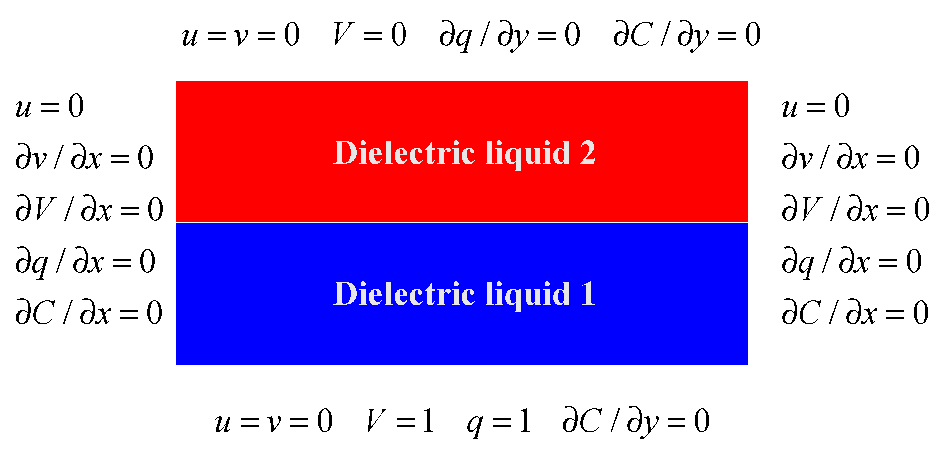
2.4. Initial and Boundary Conditions

Initially, the fluid is at rest and all variables (velocity, pressure, charge density, electric potential) are set to be zero. The concentration C for the reference liquid, the upper layer, is set to one. For the second liquid (lower layer), it set to zero. The dimensionless boundary conditions are classical and are described in Figure 2.

3. Results and Discussions

This study aims at defining how the mixing of the two dielectric liquids may be controlled and enhanced by electro-convection. Our investigations focused, too, on examining the development of the electro-convective instability in relation to the evolution of certain parameters such as the Schmidt number, the electric Rayleigh number, and the permittivity and ionic mobility ratios.

The strong injection is considered and the non-dimensional parameters C_inj are taken as 10. The mobility parameter M is also taken as 10.

The solutal Rayleigh number, Ra_S, is chosen between 100 and 20000. The electric Rayleigh number T can vary from 0 to 185.

Different permittivity and ionic mobility ratios are considered ${\epsilon }_{ratio}\in \left[0.25,10\right],K_{ratio}\in \left[0.25,10\right]$. The dynamic viscosity ratio is set to ${\mu }_{ratio}=1$.

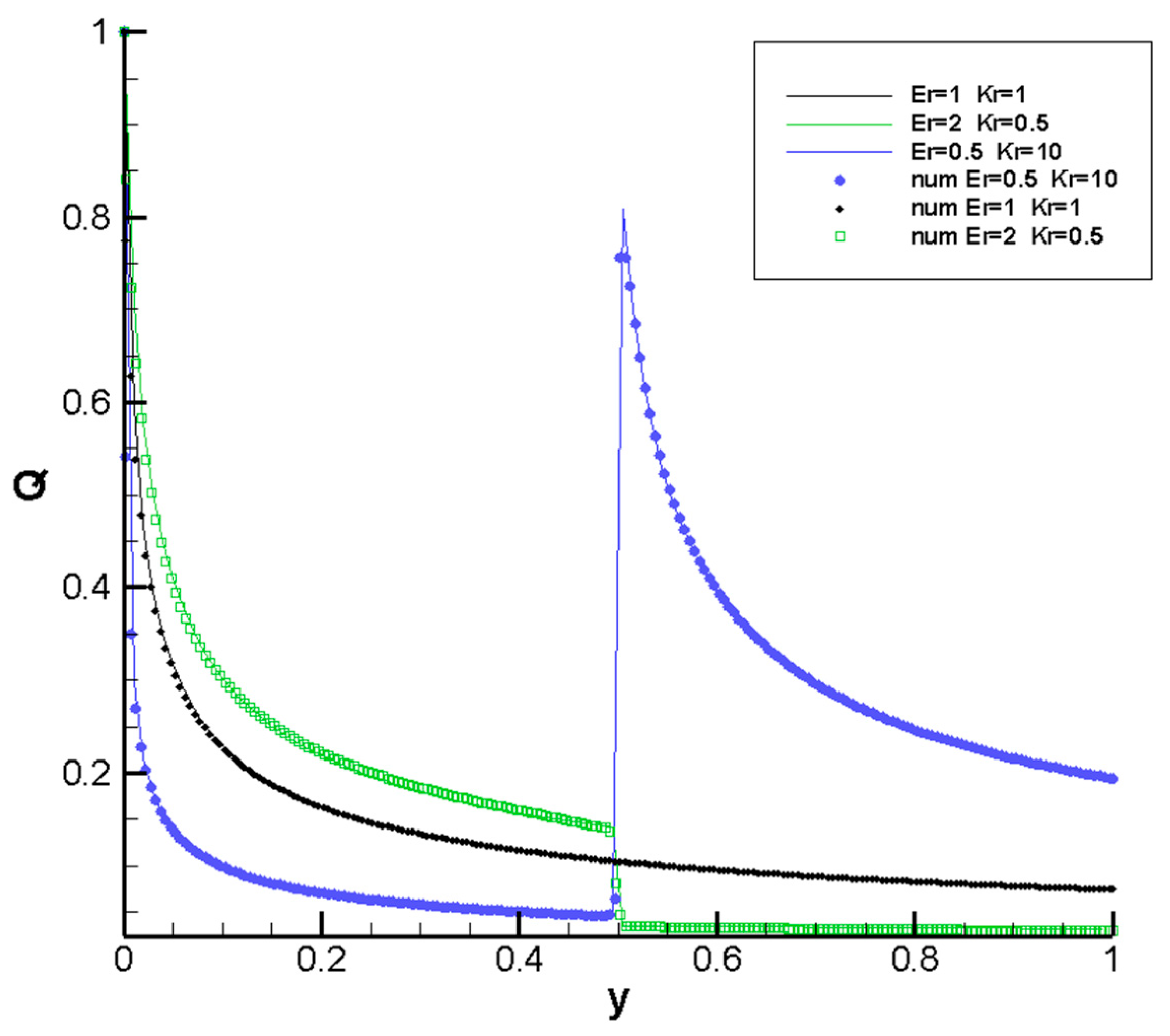
3.1. Code Validation

The code used for these simulations has been thoroughly validated through many tests and benchmarks [11,13,14]. Comparisons with analytical solution of the hydrostatic case for charge injection in a pure dielectric liquid as well as the determination of the linear and non-linear stability criteria have been undertaken. The new feature that needed to be validated was the code’s ability to simulate cases with varying density, viscosity, permittivity, and ionic mobility. There is an analytical solution for the hydrostatic case of the charge density between two layers of the liquid with different permittivity and different ionic mobility. The hydrostatic case relates to the scenario where charge injection does occur but without inducing any fluid motion. In this simplified case, an analytical solution is tractable.

The charge density distribution is given by Equations (21) and (22) see Figure 3.

Coefficient b is the solution of the equation:

$${\displaystyle \frac{4}{3}}{\displaystyle \frac{C_{inj}}{{\epsilon }_{ratio}}}{(b-h)}^{1/2}\left(b^{3/2}-{(b-h)}^{3/2}+\sqrt{K_{ratio}{\epsilon }_{ratio}}\left[{\left(h+{\displaystyle \frac{{\epsilon }_{ratio}}{K_{ratio}}}b\right)}^{3/2}-{\left({\displaystyle \frac{{\epsilon }_{ratio}}{K_{ratio}}}b\right)}^{3/2}\right]\right)-1=0$$

(23)

Equation (23) is solved by Newton–Raphson root-finding methods. Once coefficient b is determined, coefficients a, c and d are given by

$$a={\displaystyle \frac{2}{{\epsilon }_{ratio}}}{C}_{inj}{(b-h)}^{1/2} ; c={\left(K_{ratio}{\epsilon }_{ratio}\right)}^{1/2}a ; d={\displaystyle \frac{{\epsilon }_{ratio}}{K_{ratio}}}b$$

Then, the charge density distribution in the two layers is fully determined.

Figure 4 shows the comparison between the analytical and numerical solutions for three different ${\epsilon }_{ratio} \mathrm{and} K_{ratio}$. We can notice a perfect agreement between the numerical solutions and the analytical ones.

3.2. Mixture Controled by Electro-Convection

To quantify the mass transfer rate in the flow domain, we have introduced the Lacey mixing index [15]. This mixing index is defined as follows:

$${\sigma }^2={\displaystyle \frac{1}{N_{cells}}}{\displaystyle \sum _{i=1}^{N_{cells}}{(C_i-C_m)}^2}$$

(24)

where $C_i$ represents the concentration of liquid 1 in the cell i. $C_m$ is the mean expected concentration in the domain. It is equal to 0.5 as the two liquids layers have the same initial volume. $\sigma$ is the degree of mixing and represents the RMS of the deviation of the concentration from the mean value $C_m$. When the mixture is totally homogenous, $\sigma =0$.

We have computed the evolution of the Lacey index vs. time for different parameters.

3.2.1. Effect of Electro-Convection on the Mixing

Please note that from Figure 5, Figure 6, Figure 7, Figure 8, Figure 9 and Figure 10, the time as well as all quantities displayed are dimensionless. In Figure 5, we have plotted the evolution of Lacey index vs. time. We can observe two parts in this curve. Each part is defined by a certain slope. The first slope (blue) indicates that the two liquids mix solely through molecular diffusion. As the diffusion coefficient D increases, the Schmidt number S_c decreases, resulting in an increase in the first slope (blue). When the electric Rayleigh number T increases, the second slope (red) also increases. At T = 0, there is no electro-convection, so the two fluids mix purely via molecular diffusion. When T exceeds the critical value T_c = 164, electro-convective cells begin to emerge, significantly enhancing the mixing of the two fluids. As soon as T > T_c increases, the second slope (red) becomes steeper.

In Figure 6a, we plotted the evolution of the Lacey index over time, highlighting the onset of electro-convection, which occurs precisely at t = 107.65, as indicated by the red arrow. Figure 6b illustrates the maximum velocity V_max over time to demonstrate the development of electro-convective instability for T = 175 and T = 0. For T = 0 (flat red curve), we observe no movement in the liquid, confirming that mixing occurs solely through pure molecular diffusion. Figure 6c presents the stability diagram, where we have plotted the maximum velocity V_max at a steady state against different values of the T parameter. We observe that the linear critical value T_c for which electro-convection occurs, in this case, is slightly higher than the classical value T_c = 164 for homogeneous liquids. Investigations are currently underway to explain this discrepancy between homogeneous and non-homogeneous liquids.

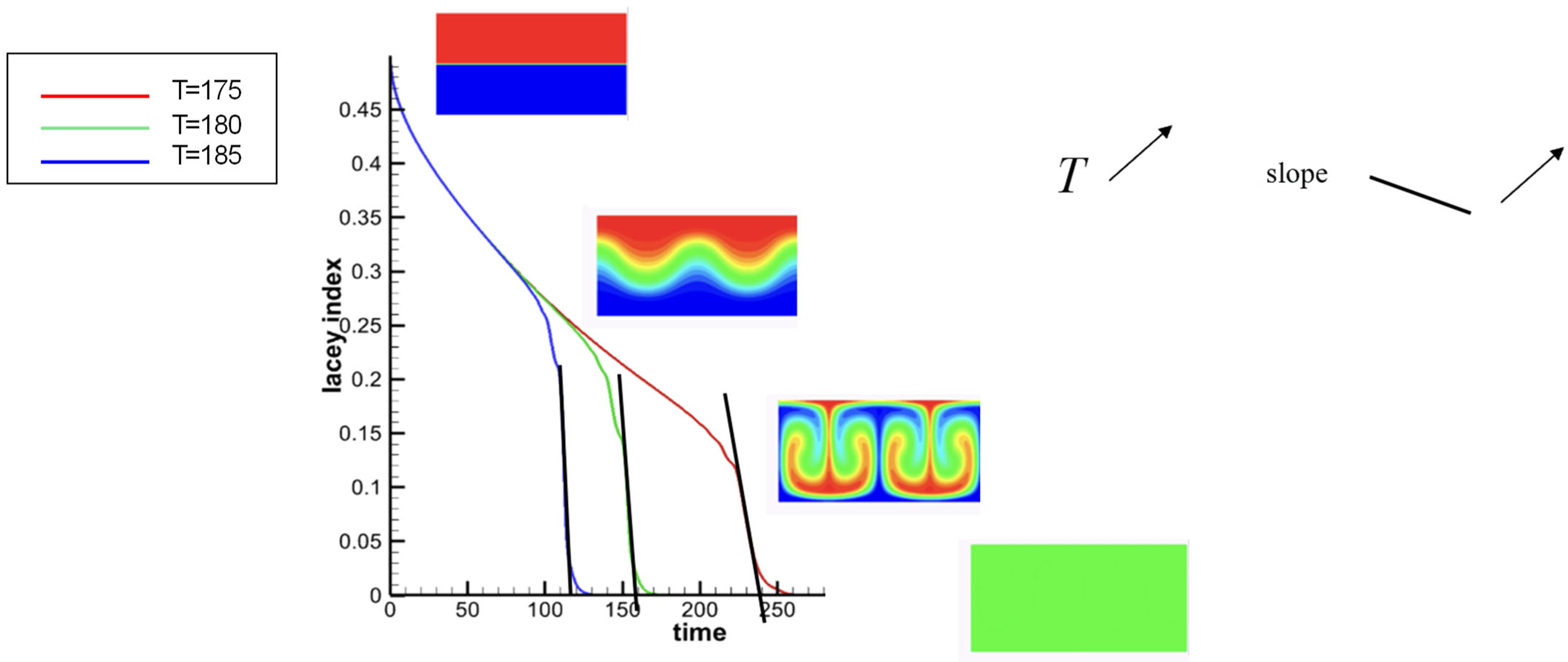
3.2.2. Effect of T on the Mixing

As anticipated, as the electrical Rayleigh T increases, meaning there is an increase in the applied voltage, the onset of electro-convection occurs earlier. Consequently, the mixture reaches a homogeneous state in a shorter period of time.

In Figure 7 we have plotted the evolution of the Lacey index vs. time for different values of T. As T increases, the two liquids achieve a state of homogeneity more rapidly. Additionally, as previously noted, the greater the T, the steeper the slope becomes. We have also depicted the different states of the concentration distribution along the time.

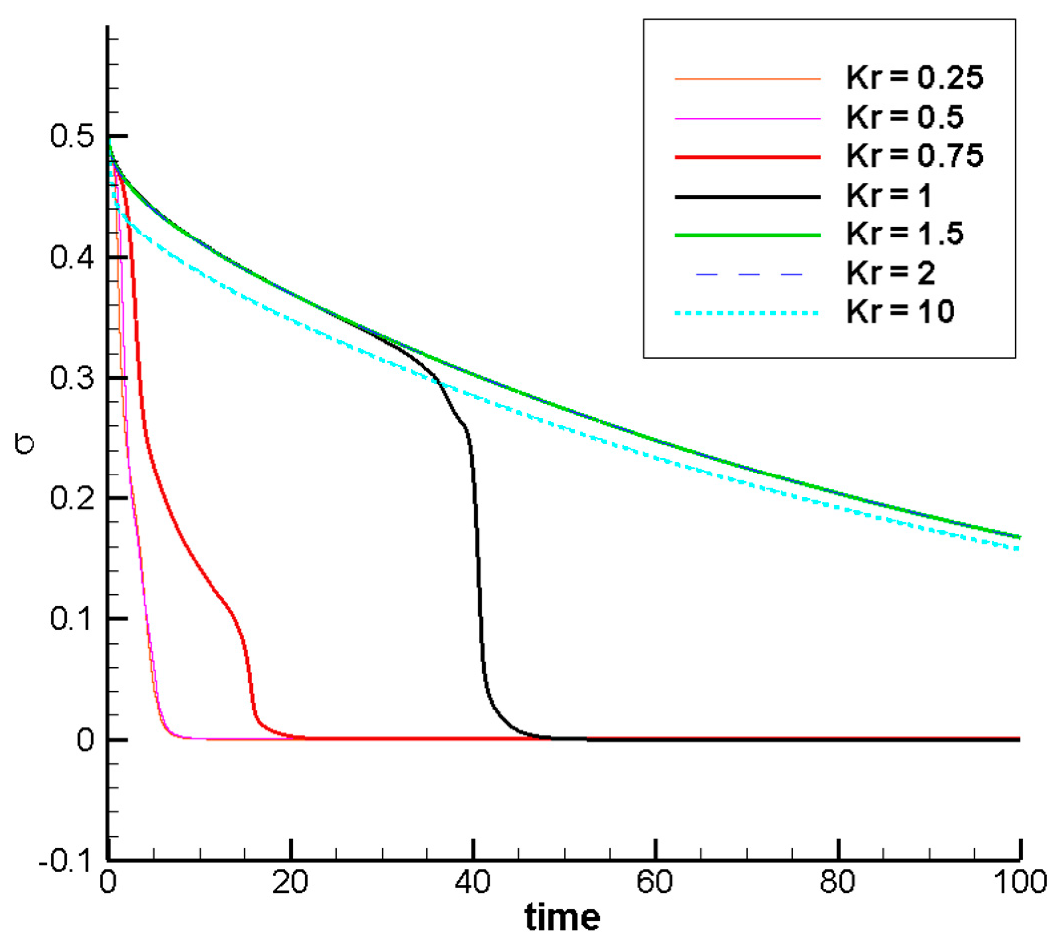
3.2.3. Effect of the Ionic Mobility Ratio on the Mixing

This effect is confirmed by Figure 8, where we depicted the evolution of Lacey index, which is a measure of the mixing degree between the two fluids.

The effective $T$ is defined as

$$\tilde{T}=T{\displaystyle \frac{2\left(1+{\epsilon }_{ratio}\right)}{\left(1+{\mu }_{ratio}\right)\left(1+K_{ratio}\right)}}={\displaystyle \frac{2T}{1+K_{ratio}}} (\mathrm{as} {\epsilon }_{ratio}=1 ; {\mu }_{ratio}=1).$$

So, when liquid 2 has a higher ionic mobility than liquid 1, i.e., $K_{ratio}>1$, the effective T is decreased. For $K_{ratio}$ equal to 1.5, 2 and 10, $\tilde{T}<T_C$ and electro-convection does not occur, thus reducing the mixing between the two liquids.

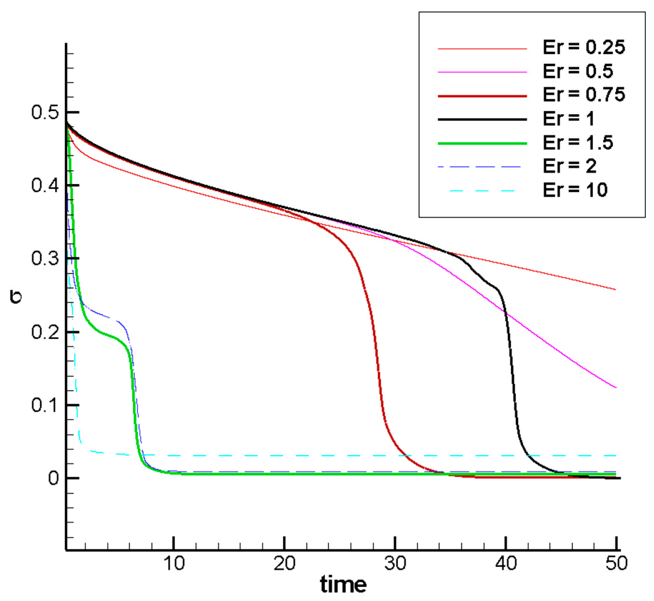
3.2.4. Effect of the Permittivity Ratio on the Mixing

This time, as $K_{ratio}=1 ; {\mu }_{ratio}=1$: $\tilde{T}=T{\displaystyle \frac{2\left(1+{\epsilon }_{ratio}\right)}{\left(1+{\mu }_{ratio}\right)\left(1+K_{ratio}\right)}}=T{\displaystyle \frac{\left(1+{\epsilon }_{ratio}\right)}{2}}$

Therefore, when liquid 2 has a higher permittivity than liquid 1, i.e., ${\epsilon }_{ratio}>1$, the effective T is increased. For ${\epsilon }_{ratio}$ equal to 1.5, 2, and 10, the effective T is strongly increased as $\tilde{T}$ is largely over T_C. Electro-convection is stronger for large ${\epsilon }_{ratio}$.

Conversely, for ${\epsilon }_{ratio}$ equal to 0.25, electro-convection does not occur since $\tilde{T}<T_C$ and the mixing between the two liquids occurs only by molecular diffusion.

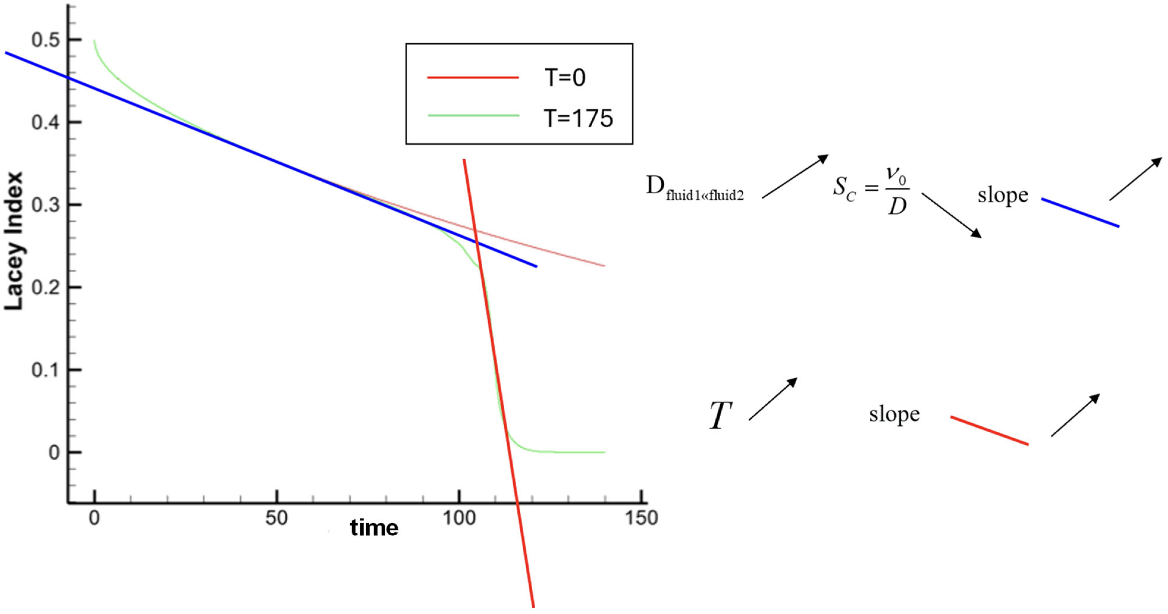
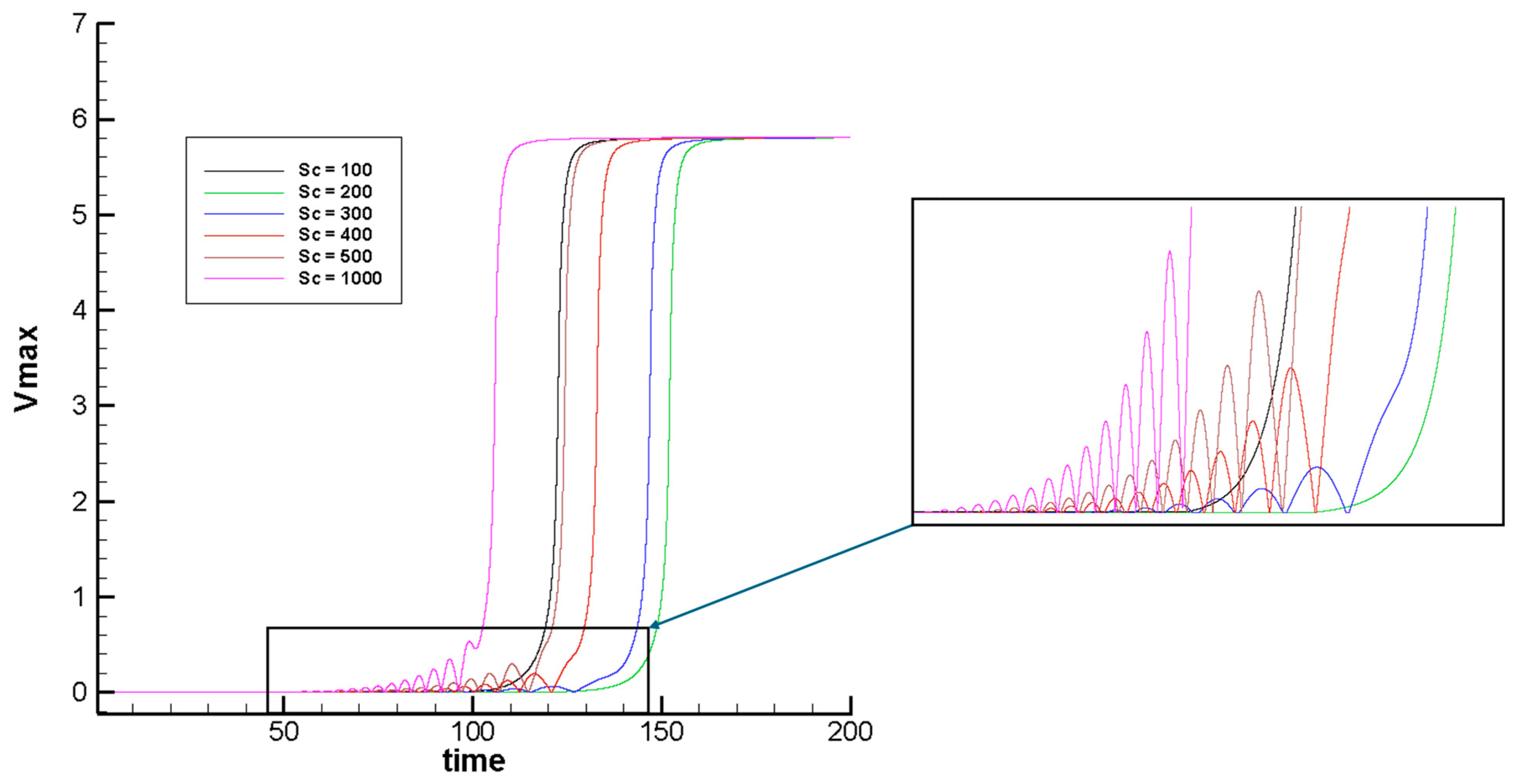
3.3. Impact of Mixing on Flow Stability

Oscillation of the Growing Instability

Our investigation focused on the development of electro-convective instability. Vmax represents the peak velocity within the fluid domain at any given moment. We charted this maximum velocity (Vmax) against time for varying Schmidt numbers, maintaining a constant T = 175, as depicted in Figure 10. For these simulations, ${\epsilon }_{ratio}=1 \mathrm{and} K_{ratio}=1$.

The plot reveals a fascinating feature which has never been reported to the best knowledge of the authors: We observe the emergence of ripples during the early stages of instability growth. These ripples are a result of the density disparity between the two liquid layers. Gravity acts as a restorative force, striving to level the interface between the two layers once it distorts.

The physical mechanism can be described as follows: The lighter liquid is placed above a heavier one, which creates a stable configuration. The motion of the fluid, driven by electro-convection and fluid inertia, causes the interface between the two liquids to deform. This deformation pushes the lighter liquid downwards and the heavier liquid upwards, see Figure 11. However, gravity acts as a restoring force, attempting to flatten the interface. This competition between inertia and gravity results in an oscillation of the interface

The oscillation frequency and amplitude are determined by the interplay between this restorative force and the liquid’s inertia induced by the emerging electro-convection.

This mechanism contributes to the EHD instability, leading to oscillations of escalating amplitude. It’s noteworthy that the amplitude and period of these ripples are influenced by the Schmidt number and the electrical Rayleigh number T.

Indeed, as the Schmidt number decreases, the system increasingly aligns with a homogeneous situation. This is because the two fluids merge rapidly into each other, resulting in a homogeneous liquid almost instantaneously. In such a scenario, the trajectory of Vmax over time closely mirrors that of the “single-phase” case, where no ripples are noted. Conversely, as the Schmidt number increases, the diffusion of the two liquids into each other reduces. This keeps the interface between the two liquids more pronounced and sharp. In such a situation, the influence of gravity remains more prevalent for an extended period.

4. Semi-Analytical Model

In this section, we describe a semi-analytical model that helps to understand the physical origin of the amplitude oscillations at the beginning of the instability. The model is in the wake of those proposed by Félici [16], Atten [10], and Castellanos [17] (see also [3]). We consider the limit of zero diffusion, an infinite Schmidt number, which means that the liquids are immiscible. Also, the injection is assumed to be weak.

The non-dimensional Navier–Stokes equation is

$${\displaystyle \frac{\partial \overrightarrow{u}}{\partial t}}+(\overrightarrow{u}·\nabla )\overrightarrow{u}=-\nabla p+{\nabla }^2\overrightarrow{u}+{\displaystyle \frac{C_{inj}{T}^2}{M^2}}q\overrightarrow{E}+GrC\overrightarrow{y}$$

Here, the Grasshoff number is defined as $Gr={\displaystyle \frac{R{a}_s}{S_c}}$. The Grasshoff number is finite in the limit of zero diffusion. The function C is 0 for the lower and denser liquid and 1 for the other.

The charge density is given by

$$q(x,y)={\displaystyle \frac{1}{1+\frac{T}{M^2}{C}_{inj}t(x,y)}}$$

where t is the time it takes a charge carrier to go from the injector to the point (x, y).

In the weak injection case ($C_{inj}\ll 1$), the charge density may be approximated by

$$q(x,y)\cong (1-{\displaystyle \frac{T}{M^2}}{C}_{inj}t(x,y))$$

To compute $t\left(x,y\right)$, it is necessary to solve the system of equations that determine the charge carrier trajectory:

$${\displaystyle \frac{dx}{dt}}={\displaystyle \frac{T}{M^2}}{E}_x+u_x$$

$${\displaystyle \frac{dy}{dt}}={\displaystyle \frac{T}{M^2}}{E}_y+u_y$$

In the weak injection limit, the electric field is simplified to $E_x=0$ and $E_y=1$.

Let us introduce a velocity roll of variable amplitude:

$$\overrightarrow{u}(x,y,t)=A(t){\overrightarrow{u}}_0(x,y)$$

where the vector function ${\overrightarrow{u}}_0(x,y)$ is given a priori. In order to fulfill continuity equation, it is convenient to express the velocity field as derived from a stream function, that is,

$$u_{0x}={\displaystyle \frac{\partial {\mathsf{\Psi }}_0}{\partial y}}$$

$$u_{0y}=-{\displaystyle \frac{\partial {\mathsf{\Psi }}_0}{\partial x}}$$

The linear stability problem reduces to studying the behavior of A(t) for small amplitudes. By introducing this velocity field in the Navier–Stokes equation, multiplying by ${\overrightarrow{u}}_0(x,y)$, and integrating over the whole domain, the following equation is received:

$$\left({\displaystyle \frac{dA}{dt}}{\displaystyle \iint {\overrightarrow{u}}_0· }{\overrightarrow{u}}_0 ds\right)=A{\displaystyle \iint {\overrightarrow{u}}_0· }{\nabla }^2{\overrightarrow{u}}_0 ds+{\displaystyle \frac{C_{inj}{T}^2}{M^2}}{\displaystyle \iint q{\overrightarrow{u}}_0· }\overrightarrow{E} ds+Gr{\displaystyle \iint C{u}_{0y} }ds$$

(25)

The pressure term is zero for a closed domain. For small velocity amplitudes, the time that a charge carrier needs to go from the injector to a certain position is

$$t\left(x,y\right)={\int }_0^y{\displaystyle \frac{dy}{\frac{T}{M^2}+A{u}_{0y}(x,y)}}$$

A Taylor expansion of the integrand gives the following:

$$t\left(x,y\right)={\displaystyle \frac{M^2}{T}}{\int }_0^{y}dy\left(1-{\displaystyle \frac{M^2}{T}}A{u}_{0y}\left(x,y\right)\right)$$

The charge density is then

$$q\left(x,z\right)=1-C_{inj}{\int }_0^{y}dy\left(1-{\displaystyle \frac{M^2}{T}}A{u}_{0y}\left(x,y\right)\right)$$

The last integral in Equation (25) requires a detailed comment. In the limit of no diffusion, the variable C is 1 or 0 and, therefore, the integral extends to the domain occupied by the upper liquid. The position of the interface $y=\xi (x,t)$ is related to the velocity field by the kinematic condition (see Figure 12), which physically represents that the interface is a material surface:

$${\displaystyle \frac{\partial \xi }{\partial t}}-u_y+u_x{\displaystyle \frac{\partial \xi }{\partial x}}=0$$

In the linear approximation and introducing the amplitude A,

$${\displaystyle \frac{\partial \xi }{\partial t}}=A(t)u_{0y}(x,y={\displaystyle \frac{1}{2}})$$

Therefore,

$$\iint C{u}_{0y}ds={\int }_0^{L}dx{\int }_{{\displaystyle \frac{1}{2}}+\xi }^1{u}_{0y} dy$$

After linearizing the result, this integral is proportional to ${\int }_0^{t}A\left(t\right) dt$.

Substituting the charge density into the integral Navier–Stokes equation gives

$$b{\displaystyle \frac{dA}{dt}}=a_{1}A+a_{2}T{C}_{inj}^{2}A+a_{3}Gr{\int }_0^{t}A dt$$

where the coefficients are computed from the following set of integrals:

$$b={\displaystyle \iint {\overrightarrow{u}}_0· }{\overrightarrow{u}}_0 ds$$

$$a_1={\displaystyle \iint {\overrightarrow{u}}_0· }{\nabla }^2{\overrightarrow{u}}_0 ds$$

$$a_2={\displaystyle \iint u_{0y}\left({\displaystyle \underset{0}{\overset{y}{\int }}{u}_{0y}}dy\right) }ds$$

$$a_3=-{\displaystyle \underset{0}{\overset{L}{\int }}dx{\displaystyle {\int }_{\frac{1}{2}+\epsilon u_{0y}(x,y=\frac{1}{2})}^1{u}_{0y}dy}}$$

where the result must be linearized in $ϵ$, and after linearization, we take $ϵ=1$.

As a particular choice of the velocity field, we chose the stream function:

$${\mathsf{\Psi }}_0={\displaystyle \frac{L}{2\pi }}\left(1-\cos \left(2\pi y\right)\right)\sin \left({\displaystyle \frac{\pi x}{L}}\right)$$

which corresponds to the structure of a single roll in the domain [0, L]x[0, 1] (see Figure 12).

The equation for the evolution of the amplitude of this single mode is as follows:

$$b{\displaystyle \frac{d^{2}A}{d{t}^2}}=\left(a_1+T{C}_{inj}^2{a}_2\right){\displaystyle \frac{dA}{dt}}+a_{3}GrA$$

(26)

and the values of the coefficients are

$$b={\displaystyle \frac{L^3}{4}}+{\displaystyle \frac{3L}{16}}$$

$$a_1=-{\pi }^2\left({\displaystyle \frac{3}{16L}}+{\displaystyle \frac{L}{2}}+L^3\right)$$

$$a_2={\displaystyle \frac{L}{16}}$$

$$a_3=-{\displaystyle \frac{L}{2}}$$

Equation (26) shows the role played by the difference in densities between both liquids. The last term represents a restoring force that opposes the displacement of the interface. In the absence of viscosity, the term $a_1{\displaystyle \frac{dA}{dt}}$, which represents dissipation, and the electric term, which represents the destabilizing effect, the last term will give place to pure oscillations of the frequency $\omega =\sqrt{{-a}_{3}Gr/b}$.

The solutions of the differential equation are of the form

$$A=A\left(0\right)e^{\lambda t}$$

where $\lambda$ is solution of the equation

$$b{\lambda }^2=\left(a_1+T{C}_{inj}^2{a}_2\right)\lambda +a_{3}Gr$$

Depending on the sign,

$$\mathsf{\Delta }={\left(a_1+T{C}_{inj}^2{a}_2\right)}^2+4b{a}_{3}Gr$$

The solutions are real or complex values. For $\mathsf{\Delta }<0$, we have

$$\lambda =\sigma +i\omega$$

with

$$\sigma ={\displaystyle \frac{a_1+{TC}_{inj}^2{a}_2}{2b}}$$

and

$$\omega ={\displaystyle \frac{\sqrt{-\mathsf{\Delta }}}{2b}}$$

For $\sigma >0$, perturbations grow, and the system is unstable. The linear stability threshold is

$$T_c{C}_{inj}^2=-{\displaystyle \frac{a_1}{a_2}}$$

Near this value, the frequency is, as above

$$\omega =\sqrt{-a_{3}Gr/b}$$

The transition from the rest state to convection occurs with oscillations at this frequency of increasing amplitude. When $T$ is high enough, $\mathsf{\Delta }$ becomes positive, and the oscillations disappear. The same happens if $T$ and $R{a}_s$ are low enough. Figure 13 plots the evolution of $\sigma$ and $\omega$ with $T{C}_{inj}^2$.

The effect of a finite diffusion would be to decrease the restoring gravity force. Therefore, the frequency of the oscillations will decrease. For a certain Schmidt number, the oscillations would disappear, as seen in the numerical results shown in Figure 10 and Figure 13. The number of observed oscillations is proportional to the ratio $\omega /\sigma$, since $2\pi /\omega$ is the period of oscillations and $1/\sigma$ is the typical growth time. As seen in Figure 13, above the critical value of T, $\omega$ decreases and $\sigma$ increases. Therefore, the number of oscillations decreases when T increases, as observed in numerical simulations.

5. Conclusions

This study focuses on the behavior of two parallel layers consisting of different miscible dielectric liquids within an enclosed cavity subjected to unipolar injection. A numerical model is developed to simulate the behavior of these liquids with varying physical properties when exposed to unipolar injection. The results demonstrate the remarkable enhancement of mixing between the two liquids due to electro-convection. The degree of mixing, quantified by the Lacey index, is found to be strongly dependent on the electrical Rayleigh number, as expected. One intriguing finding of this research is the emergence of oscillations in the two liquid layers during the early stages of electro-convective instability growth. This behavior, which has not been reported in the literature thus far, is attributed to the density disparity between the liquid layers. The motion of the fluid, driven by electro-convection and fluid inertia, causes distortion in the interface between the layers. Gravity acts as a restorative force, attempting to level this interface. The amplitude and frequency of these oscillations are found to be related to the electric Rayleigh number, Schmidt number, and the ratio of permittivity and ionic mobility. To further support the numerical findings, a semi-analytical model is developed specifically for weak injection scenarios. This model confirms the observed trends from the numerical simulations, providing additional insights into the behavior of the system. These findings contribute to a deeper understanding of the complex dynamics associated with the electro-convective instability in miscible dielectric liquids. The results have implications for various applications, including microfluidics, energy conversion, and mixing processes. Further research is warranted to explore the underlying mechanisms and optimize the control of electro-convection for practical applications.

References

1. Castellanos, A. Electrohydrodynamics; Springer: New York, NY, USA, 1999. [Google Scholar]
2. Chang, J.S.; Kelly, A.J.; Crowley, J.M. Handbook of Electrostatic Processes, 2nd ed.; Dekker: New York, NY, USA, 1995. [Google Scholar]
3. Traoré, P.; Pérez, A.T.; Koulova, D.; Romat, H. Numerical modelling of finite-amplitude electro-thermo convection in a dielectric liquid layer subjected to both unipolar injection and temperature gradient. J. Fluid Mech. 2010, 658, 279. [Google Scholar] [CrossRef]
4. Wu, J.; Traoré, P.; Zhang, M.; Pérez, A.T.; Vázquez, P.A. Charge injection enhanced natural convection heat transfer in horizontal concentric annuli filled with a dielectric liquid. Int. J. Heat Mass Transf. 2016, 92, 139–148. [Google Scholar] [CrossRef]
5. Wu, J.; Traoré, P.; Louste, C.; Pérez, A.T.; Vázquez, P.A. Numerical evaluation of heat transfer enhancement due to annular electroconvection induced by injection in a dielectric liquid. IEEE Trans. Dielectr. Electr. Insul. 2016, 23, 614. [Google Scholar] [CrossRef]
6. Jalaal, M.; Khorshidi, B.; Esmaeilzadeh, E. Electrohydrodynamic (EHD) mixing of two miscible dielectric liquids. Chem. Eng. J. 2013, 219, 118–123. [Google Scholar] [CrossRef]
7. Heidari, R.; Khosroshahi, A.R.; Sadri, B.; Esmaeilzadeh, E. The Electrohydrodynamic mixer for producing homogenous emulsion of dielectric liquids. Colloids and Surfaces A Physicochemical and Engineering Aspects 2019, 578, 123592. [Google Scholar] [CrossRef]
8. Chicon, R.; Castellanos, A.; Martin, E. Numerical Modelling of Coulomb-driven Convection in Insulating Liquids. J. Fluid Mech. 1997, 344, 43–66. [Google Scholar] [CrossRef]
9. Atten, P.; Moreau, R. Stabilité électrohydrodynamique des liquides isolants soumis à une injection unipolaire. J. Mécanique 1972, 11, 471. [Google Scholar]
10. Atten, P.; Lacroix, J.C. Non-linear hydrodynamic stability of liquids subjected to unipolar injection. J. Mécanique 1979, 18, 469. [Google Scholar]
11. Traoré, P.; Pérez, A.T. Two-dimensional numerical analysis of electroconvection in a dielectric liquid subjected to strong unipolar injection. Phys. Fluids 2012, 24, 037102. [Google Scholar] [CrossRef]
12. Liang, X.; Wang, L.; Li, D.; Ma, B.; He, K. Lattice Boltzmann modeling of double-diffusive convection of dielectric liquid in rectangular cavity subjected to unipolar injection. Phys. Fluids 2021, 33, 067106. [Google Scholar] [CrossRef]
13. Wu, J.; Traoré, P. A finite-volume method for electrothermoconvective phenomena in a plane layer of dielectric liquid. Numer. Heat Transf. Part A 2015, 68, 471–500. [Google Scholar] [CrossRef]
14. Traoré, P.; Wu, J. On the limitation of Imposed Velocity Field strategy for Coulomb-driven electroconvection flow simulations. J. Fluid Mech. 2013, 727, R3. [Google Scholar] [CrossRef]
15. Mondal, S.; Traore, P.; Bhattacharya, A.; Perez, A.T.; Vasquez, P.A. Mass Transfer Enhancement Induced by Electro Soluto Convection within two Parallel Electrodes Due to unipolar Charge Injection. In Proceedings of the 2022 IEEE 21st International Conference on Dielectric Liquids (ICDL), Sevilla, Spain, 25 May–2 June 2022. [Google Scholar]
16. Félici, N. Phenoménes hydro et aérodynamiques dans la conduction des diélectriques fluides. Rev. Gén. Electr. 1969, 78, 717–734. [Google Scholar]
17. Castellanos, A. Coulomb driven convection in electrohydrodynamics. IEEE Trans. Electr. Insul. 1991, 26, 1201–1215. [Google Scholar] [CrossRef]
Figure 1. Schematic diagram of the problem. (a) General electric configuration. (b) Physical properties of each liquid.
Fluids 09 00219 g001
Figure 2. Boundary conditions.
Fluids 09 00219 g002
Figure 3. Hydrostatic solution in the two layers.
Fluids 09 00219 g003
Figure 4. Comparison between analytical vs. numerical solution of the hydrostatic case for different ε r a t i o   and   K r a t i o .
Fluids 09 00219 g004
Figure 5. Mixing index vs. time for T = 0 and T = 175: evolution of the two slopes.
Fluids 09 00219 g005
Figure 6. (a) Mixing vs. time for T = 0 and T = 175: identification of electro-convection start with Vmax vs. time (b) and Vmax vs. T (c).
Fluids 09 00219 g006
Figure 7. Influence of T on the mixing of the liquids. The structure of the concentration field is displayed along the curve to show the structure of the flow at given instants. As T is increased the slope of the curve increases.
Fluids 09 00219 g007
Figure 8. Lacey index vs. time for different K R a t i o values, T = 190, Sc = 1000.
Fluids 09 00219 g008
Figure 9. Lacey index vs. time for different ε R a t i o values, T = 190, Sc = 1000.
Fluids 09 00219 g009
Figure 10. Evolution of Vmax vs. time for different Schmidt numbers. T = 175, ε r a t i o = 1   K r a t i o = 1 .
Fluids 09 00219 g010
Figure 11. Physical mechanism and electro-convective motion.
Fluids 09 00219 g011
Figure 12. Velocity and interphase separation for small-amplitude motion.
Fluids 09 00219 g012
Figure 13. (a): Growth rate (red line) and frequency (blue line) as a function of the electric parameter. The circle marks the stability threshold. (b): Zoom of the figure near the stability limit.
Fluids 09 00219 g013
Disclaimer/Publisher’s Note: The statements, opinions and data contained in all publications are solely those of the individual author(s) and contributor(s) and not of MDPI and/or the editor(s). MDPI and/or the editor(s) disclaim responsibility for any injury to people or property resulting from any ideas, methods, instructions or products referred to in the content.