Turbulent Micropolar Open-Channel Flow

Abstract

The present paper focuses on the investigation of the turbulent characteristics of an open-channel flow by employing the micropolar model. The underlying model has already been proven to correctly describe the secondary phase of turbulent wall-bounded flows. The open-channel case comprises an ideal candidate to further test the micropolar model as many environmental flows carry a secondary phase, the behavior of which is of great interest for applications such as sedimentation transport and debris flow. Direct Numerical Simulations (DNSs) have been carried out on an open channel for $R{e}_b$ = 11,200 based on mean crossectional velocity, channel height, and the fluid kinematic viscosity. The simulated results are compared against previous experimental as well as Langrangian DNS data of similar flows, with excellent agreement. The micropolar model is capable of describing the same problem but in an Eulerian frame, thus significantly simplifying the computational cost and complexity.

1. Introduction

Open-channel particulate flows is a demanding field of research which, similarly to many natural processes, requires significant effort to investigate numerically. The complexity of the problem lies in the effort to establish a multiparametric model to accurately describe as many of its physical counterparts as possible. This general type of flow applies to several cases of environmental and industrial flows. Typical examples of open-channel particulate flows include river flows, which, in turn, entail sediment transport or industrial processes and the transportation of granular materials. As can be easily understood from these examples, particle deposition as well as the general behavior of the secondary phase plays a crucial role in the physical development of the flow.

Particle interactions with the flow, especially in the vicinity of the wall, can be very difficult to model. In many cases, the behavior of small scale turbulent structures may be altered, leading to phenomena such as turbulence enhancement or attenuation. Particle–turbulence interactions in an open-channel flow have been the main subject of numerous experimental and numerical studies in recent decades, with the results still being controversial. Early experimental studies have pointed out the importance of the interactions occurring between particles and turbulence structures in the near-wall region [1,2,3].

In the original experiments of Rashidi et al. [1], two different particle sizes were considered, where different effects were observed for each case. Particles with a larger diameter led to increased turbulence intensities and Reynolds stresses, while smaller size particles led to opposite phenomena. Apart from the particle size, another critical parameter is the concentration of the dispersed phase. Kulick et al. [4] examined the effect of different particle loadings in the two-phase flow and how this parameter could alter the turbulent characteristics. They reached the conclusion that, as particle mass loading increases, turbulence attenuation is observed, a phenomenon that is more pronounced in the transverse flow direction.

From the examples given above, it can be easily understood that the dispersed phase adds complexity to the problem, even in straight open-channel flows. Apart from those mentioned above, other particle characteristics that may influence the flow properties are the degrees of freedom and the spin gradient or inertia properties, many of which are quite cumbersome to measure experimentally. Therefore, many studies have tried to approach the problem numerically, either through Direct Numerical Simulations or by utilizing a turbulence model [5,6,7,8,9]. Once again, these studies have revealed interesting phenomena regarding the interaction of particles with the carrier flow concerns. Dritselis and Vlachos [6] adopted a point-force model in order to examine the effect of small heavy particles on the flow, without finding any evidence of qualitative velocity changes due to particle presence. On the other hand, they pointed out that near-wall velocity-coherent structures seem to be directly affected by the rotational motion of the dispersed particles. Another important parameter that affects the flow phenomena is the clustering and dispersion of the secondary phase, especially close to the bottom-wall area [10,11].

Finally, in the comparative analysis of Yu et al. [12], various studies with controversial results were examined. The controversy of the studies that the authors examined concerned the velocity lag between the laden and unladen flow, as well as the effect of the dispersed phase on the von Kármán velocity distribution constant. In their analysis, they concluded that the addition of particles in the flow should lead to mixed behavior as far as the velocity distribution is concerned; hence, the von Kármán is constant. In the inner region, the velocity values of the particulate flow surpass the respective unladen ones, while in the outer region the exact opposite behavior should be observed.

In the majority of the above mentioned numerical studies, Lagrangian methods have been utilized in order to model the two-phase flow. Although these methods have been well-validated throughout the years, they still require considerable computational resources due to the additional number of equations that need to be solved. Moreover, the increased problem complexity leads to many additional model parameters, which in many cases are difficult to solve. Thus, an Eulerian approach to modeling the particulate phase in the special case of an open-channel flow would have obvious advantages, in terms of speed and accuracy, as well as reduced parameter complexity, provided that it is successfully verified. Eulerian approaches come with some limitations as well, when compared to Lagrangian ones. Although the Eulerian approach is able to take into account the physics of the secondary phase and describe its impact on the general flow physics, it cannot accurately describe particle motion.

A well-documented Eulerian model that is capable of modeling particulate flows is the micropolar model, which has been originally mathematically introduced by Eringen [13] and successfully applied to turbulent wall-bounded (Poiseuille) flows [14,15]. The micropolar model takes into account characteristics of the dispersed phase such as spin gradient, inertia, and particle viscosity but in an Eulerian frame of reference. Since several studies still present conflicting results regarding even the first-order properties of the flow [12], such as the velocity lag between the laden and unladen flow, alternative approaches, like the micropolar model, would be beneficial. The micropolar model comprises an invaluable computational asset for the present problem, capable of diving deep into both the macroscopic and particle properties, without complex modeling requirements.

The idea of the micropolar model being applied to environmental flows has already been revised, e.g., refs. [16,17]. Bender et al. [16] have introduced a novel Smoothed Particle Hydrodynamics (SPH) micropolar model in order to perform numerical simulations of turbulent environmental flows. The results of their study are in good agreement with the literature, without the simulations presenting computational overhead. In addition, Bender et al. [16] have incorporated the micropolar model in combination with the Discrete Element Method (DEM) to perform simulations on the OpenFOAM CFD platform. Their numerical simulations of two-phase geological flows, with particles of different sizes, were successful, with the results once again being encouraging.

In this study, the micropolar model is exploited for the first time to study a typical case of environmental flows, the turbulent open-channel flow, in combination with fully resolved Direct Numerical Simulations (DNSs). The results of the unladen case have been firstly validated against respective experimental as well as computational ones, taken from well-documented previous studies. In most cases, the present micropolar model achieves better predictions of the flow characteristics compared to existing models in the literature. Furthermore, a case of high micropolar viscosity value, which accounts for a particulate flow, has been examined and compared once again with previous data. The results of the micropolar case seem very encouraging, while the model is able to capture the usual flow characteristics of a particulate flow, giving, in some cases, better physical explanation of the underlying phenomena.

The present paper is organized as follows. The governing equations of the micropolar model, as well as the specifications of the geometry and numerical modeling, are given in Section 2. The results and discussion, which include the validation and comparison against experimental and computational data, are presented in Section 3. Useful conclusions and comments are finally presented in Section 4.

2. Materials and Methods

2.1. Governing Equations

The numerical modeling of the present study has been kept in alignment with previous DNS studies in micropolar channel flows [14,15]. In this sense, the governing equations included the continuity and micropolar linear and angular momentum equations, as originally proposed by Eringen [13].

$$\nabla \times \mathbf{u}=0$$

(1)

$${\displaystyle \frac{\partial \mathbf{u}}{\partial t}}+\left(\mathbf{u}\times \nabla \right)\mathbf{u}=-\nabla P+{\displaystyle \frac{1}{Re}}{\nabla }^2\mathbf{u}+{\displaystyle \frac{m}{Re}}\nabla \times \mathbf{\omega }$$

(2)

$${\displaystyle \frac{JN}{m}}\left({\displaystyle \frac{\partial \mathbf{\omega }}{\partial t}}+(\mathbf{u}\times \nabla )\mathbf{\omega }\right)={\displaystyle \frac{1}{Re}}{\nabla }^2\mathbf{\omega }+{\displaystyle \frac{N}{Re}}\nabla \times \mathbf{u}-2{\displaystyle \frac{N}{Re}}\mathbf{\omega }$$

(3)

In Equations (1)–(3), the usual variable of t has been selected to represent time, while two different velocity representations are present. The angular flow velocity, which is also present in the original equation description of Eringen [13], is represented here by $\mathbf{\omega }$. Moreover, the classic linear velocity vector and pressure are represented by $\mathbf{u}$ and P, respectively. For a detailed derivation of Equations (1)–(3), the interested reader is referred to the Appendix of Sofiadis and Sarris [14].

In order to arrive at the non-dimensional state of the governing set of Equations (1)–(3), a characteristic length ($\delta$) has been chosen. The total height of the channel is set to be equal to $h=2\delta$, while the characteristic velocity and density are denoted by $U_0$ and ${\rho }_0$, respectively, where the zero subscript indicates average quantities.

For the open-channel case that is presented in this study, the Reynolds number depends on the channel total height and flow total viscosity and is defined as $R{e}_h={\displaystyle \frac{\rho U_{0}h}{\mu +\kappa }}$, while this can be rewritten in terms of ($2h$) as $R{e}_b={\displaystyle \frac{\rho U_{0}2h}{\mu +\kappa }}$. The sum of $\mu$ and $\kappa$ represents the flow total viscosity (${\mu }_t$), with $\mu$ being the molecular and $\kappa$ the micropolar one. The rest of the non-dimensional parameters are $m={\displaystyle \frac{\kappa }{\mu +\kappa }}$ the vortex viscosity parameter; $J={\displaystyle \frac{j}{{\delta }^2}}$ the dimensionless microrotation based on ${\delta }^2$, where j is the microinertia of the fluid; and $N={\displaystyle \frac{\kappa {\delta }^2}{\gamma }}$ the spin gradient viscosity parameter, where $\gamma$ is the material coefficient of the fluid. Parameter values of $N=8.3\times {10}^4$ and $J=1\times {10}^{-5}$ have been kept constant throughout the present study.

In the general micropolar theory, (C) is a couple stress tensor that represents the internal moments in the material. More specifically, it describes the distribution of rotational forces within the material [13]. In other words, (C) captures the resistance of the material to bending and twisting deformations and represents the moments per unit area within the material that arise due to the internal microstructure’s resistance to rotation or torsion. In the specific isotropic case, such as the one that is considered here, the second-order tensor can be reduced into a scalar. From this equation, following the appropriate non-dimensionalization, the micropolar viscosity ratio (m) can be derived. A detailed derivation of the above can be found in the Appendix of Sofiadis and Sarris [14]. Different particle sizes and densities can be found in natural sediment transport and industrial processes. This diversity of internal microstructure characteristics results in different distributions of rotational forces within the material. The latter can be successfully described by micropolar theory; the couple stress tensor (C); and, subsequently, (m). All of the above is considered in an Eulerian frame of reference, which is one of the major advantages of micropolar theory.

The mean force rate is kept constant in the present simulations, which corresponds to a fixed value of mean mass flow rate and leads to a fixed $R{e}_b$. On the other hand, the pressure gradient is calculated and corrected in every time step. Finally, in the analysis of computed results, flow variables have been scaled according to wall coordinates. This has been achieved through the calculation of wall-shear velocity, $u_{\tau }=\sqrt{{\displaystyle \frac{{\tau }_w}{\rho }}}$, where ${\tau }_w={\mu }_t{\left({\displaystyle \frac{\partial <u>}{\partial y}}\right)}_w$ is the shear stress at the wall and <$\mathbf{u}$> denotes the mean velocity value with respect to time (t) and space. As a consequence, the friction Reynolds number can be written as $R{e}_{\tau }={\displaystyle \frac{u_{\tau }h}{\nu }}$, which in the present study corresponds to a value of $R{e}_{\tau }=330$ for the choice of $R{e}_b$ = 11,200. After being non-dimensionalized, Equations (1)–(3) have been implemented in the open-source CFD platform OpenFOAM, where they have been solved directly followed by appropriate boundary conditions for the open-channel case. The OpenFOAM solver that we depart from in order to obtain the micropolar model is the solver icoFoam. The code is available upon request to the authors.

2.2. Numerical Schemes

The discretized governing set of Equations (1)–(3) has been advanced with up to third-order accurate schemes in space (Gauss Cubic scheme), and a second-order accurate implicit backward scheme in time. These schemes consist the standard approach of the OpenFOAM platform for the case of DNS modeling and have been previously validated against benchmark cases. Additionally, they have proven to produce accurate results along with the micropolar algorithm for the wall-bounded channel case [14,15]. The coupling of momentum with pressure has been achieved through the pressure-implicit split-operator (PISO) method. This algorithm follows an iterative procedure, where the pressure equation is solved twice and the mass conservation is enforced with an explicit correction to velocity so that momentum conservation is satisfied.

In order to obtain transient free results (statistically independent), the present paper simulations have been integrated in time for up to 10 eddy turn-over times starting from arbitrary turbulent initial conditions. A perturbation has been implemented in the initial flow field in order to create these arbitrary turbulent initial conditions. As soon as the initial criteria are satisfied, the statistics of all quantities are obtained for several eddy turn-over times until statistical stationarity occurs. The averaging period corresponds approximately to a time of 15,000 $\nu /u_{\tau }^2$, where $t\nu /u_{\tau }^2$ represents the non-dimensional time unit ($t^{+}=t{u}_{\tau }^2/\nu$) [14,15]. In order to provide a standarized measure to the reader to evaluate the present model computational efficiency, the CUT (Computational Unit Time) has been utilized. This is a metric that helps with the quantification of the computational cost of a certain simulation and is calculated as CUT = (total walltime/total number of timesteps)/(total number of grid cells/number of CPU cores). In the present study, the typical CUT = 0.0013.

2.3. Model Geometry

The channel flow set-up (see Figure 1) is a common selection for open-channel turbulent flow investigation, especially with DNSs. The channel is typically represented by a rectangular cross-section with the dimensions and mesh size appropriately adjusted to the needs of the case. The computational domain size has been kept equal to $3\pi \delta$ and $2\pi \delta$ in the streamwise and spanwise periodic directions, respectively, while the total height (wall-normal direction) is set equal to $h=2\delta$. The grid resolution has been selected to be $128\times 132\times 128$ in the streamwise, wall-normal, and spanwise directions, respectively. The aforementioned grid dimensions correspond, for the non-micropolar case (m = 0), to a uniform grid spacing at the two periodic directions, streamwise and spanwise. At these two directions, wall-scaled grid spacing is equal to ${\Delta }_x^{+}=12.6$ and ${\Delta }_z^{+}=8$. One of the most demanding tasks when solving turbulent flows with Direct Numerical Simulations (DNSs) is to capture the finer scales of the flow. This task becomes particularly important in the near wall region, where very-fast-moving small eddies reside. Thus, special attention should be paid to grid clustering very close to the wall. In the present case, the choice of appropriate grid spacing in the wall-normal direction has led to a non-uniform mesh of sizes ${\Delta }_{ymin}^{+}=0.6$ and ${\Delta }_{ymax}^{+}=4.6$ is used. For the $Re$ that is investigated in the current project, the aforementioned grid resolution has been reported to be adequate in previous studies of both open and wall-bounded channels [14,15,18,19].

The boundary conditions considered in the current study include no-slip at the bottom wall and slip at the top boundary, while mean velocity has been kept constant in the streamwise direction. Periodic boundary conditions have been selected in the streamwise and spanwise directions. The velocity boundary conditions of the computational domain are summarized in

Table 1. Velocity boundary conditions prescribed to the current computational domain.

Top Plane	Free-Slip
Bottom Plane	No-Slip
Side Planes	Periodic
Inlet	Periodic
Outlet	Periodic

.

3. Results

Mean flow variables and structures have been extracted from the simulations and are presented in this section in order to analyze the flow physics.

3.1. Mean Velocity

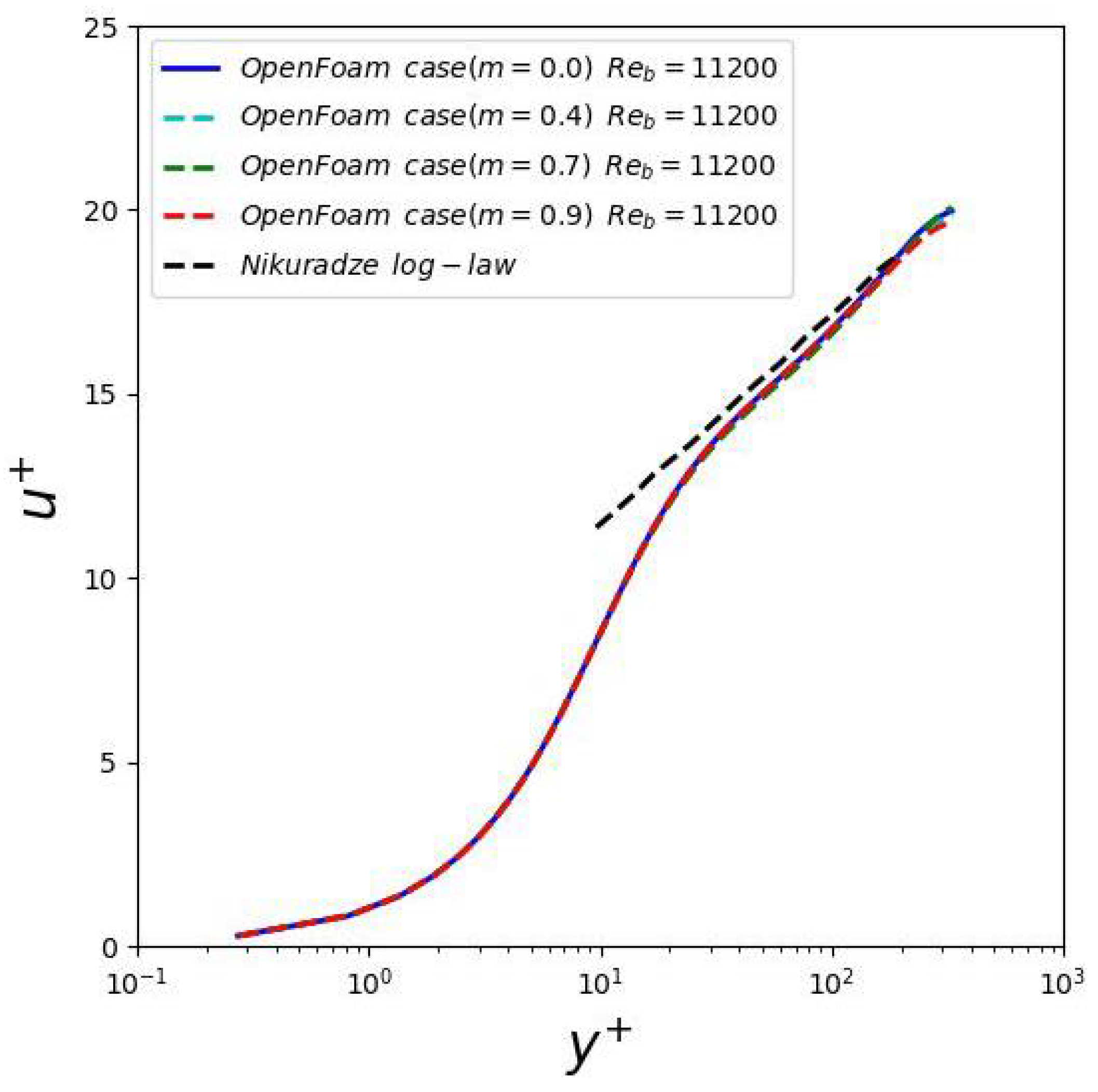
At first, the normalized hydrodynamic mean velocity profile ($u^{+}$) has been plotted along the normalized wall-distance ($y^{+}$) and compared against previous experimental and DNS data. In order to calculate the hydrodynamic data, the micropolar viscosity parameter m has been set equal to $m=0$. In this case, Equation (2) reduces to the usual Navier-Stokes one, while Equation (3) does not contribute to the solution of the system. The comparison has been conducted for the hydrodynamic case of $R{e}_b$ = 11,200 and is presented in Figure 2. The variables to which the superscript (+) has been assigned have been scaled by wall units, i.e., $y^{+}=y{u}_{\tau }/\nu$, where $\nu$ is the kinematic viscosity and $u_{\tau }$ the wall shear velocity.

The mean hydrodynamic velocity profile shows excellent agreement with previous numerical and experimental data. In Figure 2, the results of the present DNS simulation seem to converge closer to the experimental values of Komori et al. [18] than the previous DNS data of Lam and Banerjee [19]. More specifically, the maximum local error between the present results and experimental ones of Komori et al. [18] can be found at $y^{+}=4$ and is ≈27%. The small deviation from previous data is expected as the present case of $R{e}_b$ = 11,200 (based on characteristic length 2h) collapses to a value of $R{e}_{\tau }=166$ ($R{e}_{\tau }$ based on half fluid liquid depth); in the case of Komori et al. [18], it is equal to $R{e}_{\tau }=160$ ($R{e}_{\delta }=6000$, based on characteristic length $\delta$); and in case of Lam and Banerjee [19], $R{e}_{\tau }=171$ ($R{e}_b$ = 11,000). Moreover, the present DNS results have been also compared against the recent DNS results of Bauer et al. [20], where a larger domain of dimensions $Lx/h=37.7142,Lz/h=12.5664$ has been used for $R{e}_{\delta }=6340$ and $R{e}_{\tau }=200$. Nevertheless, the velocity profile curves are in good agreement with each other, as well as Nikuradze’s log-law, without violating the physical laws. It is true that the present paper uses a smaller domain and gird resolution than the study of [20], although with no obvious drawbacks. Turbulence statistics are well converged and have adequate accuracy in order to assist the comments and discussion on the flow physics.

Apart from the hydrodynamic case, an additional set of numerical simulations was conducted, which considered the micropolar formulation of the Navier–Stokes equation. The detailed formulation of these equations has been extensively described in previous studies of Sofiadis and Sarris [14,15], where the case of a wall-bounded channel flow was examined with very interesting results. In the present case, the normalized mean velocity profile has been plotted against the normalized wall distance for three different micropolar viscosity ratios $m=0.4,0.7$, and $0.9$, in Figure 3. The larger values of the micropolar viscosity ratio, close to $1.0$, characterize stronger micropolar behavior, which has been found to be analogous to a higher volume fraction in particulate flows. The rest of the non-dimensional parameters have been kept constant. The main reason for this choice is that the micropolar viscosity ratio directly affects the flow characteristics, as can be seen through the governing Equations (1)–(3). Furthermore, since this is a first application of the micropolar model to environmental flows, a study of the effect of the rest of the parameters will be conducted in future works.

The mean velocity profiles of the various micropolar cases have been plotted along with the hydrodynamic case of the same $R{e}_b$ in Figure 3. The profile curves present very small deviations between each other, indicating the very small influence of the micropolar parameters. These results, although expected, are in contrast with previous findings of the velocity profile trends in the case of wall-bounded channel flow. This behavior is attributed to the existence of the slip condition on the top-wall of the geometry. Previous studies have shown that the main influence of the micropolar part of the equations can be spotted very close to the wall Sofiadis and Sarris [14,15]. Therefore, it is expected that in the present case this influence can only be strong in the lower part of the geometry (bottom wall) and will gradually decrease as we move further away from the wall.

The maximum difference occurs between the micropolar case of $m=0.9$ and the hydrodynamic one, which is approximately of the order of $1\times {10}^{-2}$. In a relevant numerical investigation [8], it has been reported that the particle secondary phase had a negligible effect on the hydrodynamic velocity profile. In addition, the difference between the single- and two-phase flow velocity profile was in that case smaller than $9.3\times {10}^{-3}$ times the maximum velocity.

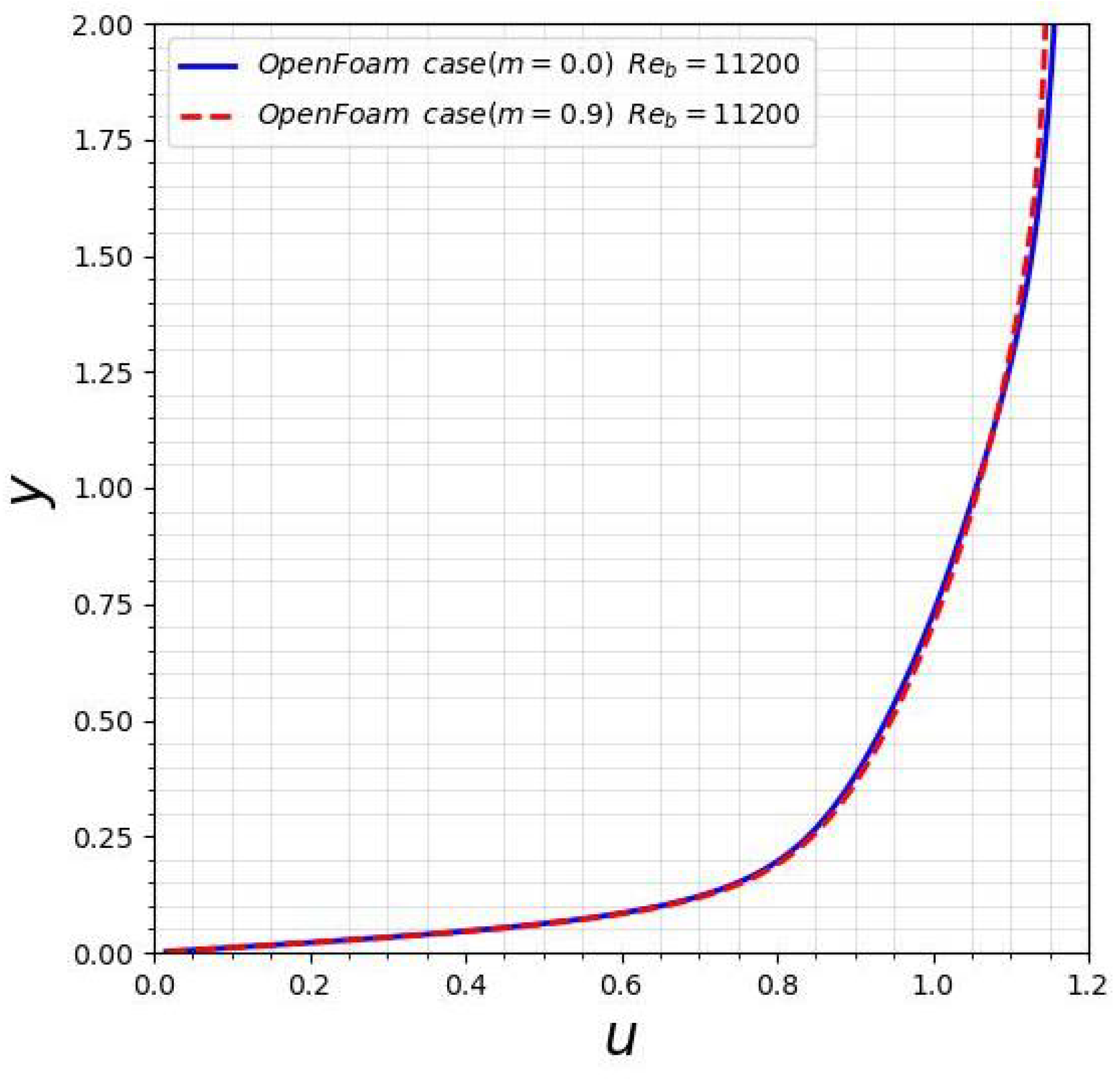
On the other hand, controversial issues found in the literature regarding the effect of the sediment phase on the mean flow velocity are presented in Yu et al. [12]. It is a fact that many researchers still argue that the sediment phase leaves the mean velocity profile mainly unchanged, and, thus, the Kármán constant has approximately the same value as in the unladen case. This idea was first proposed by Coleman [21] in his original study. Nevertheless, other studies support the original findings [22], which show a clear change in the mean flow velocity profile when the sedimentation phase is present. Finally, Yu et al. [12] concluded that, when particles are added in a turbulent open-channel flow over smooth bed, the mean flow velocity profile trend changes, though in a smaller magnitude than expected. In other words, two different behaviors should be expected. In the inner region, the unladen flow presents a smaller velocity, while in the outer region this trend is reversed, with the unladen flow moving faster than the one including sediment transport. Similar behavior is also confirmed in the present study, as can be clearly seen in Figure 4. The magnitude of change is considered in this study to depend on the sediment characteristics.

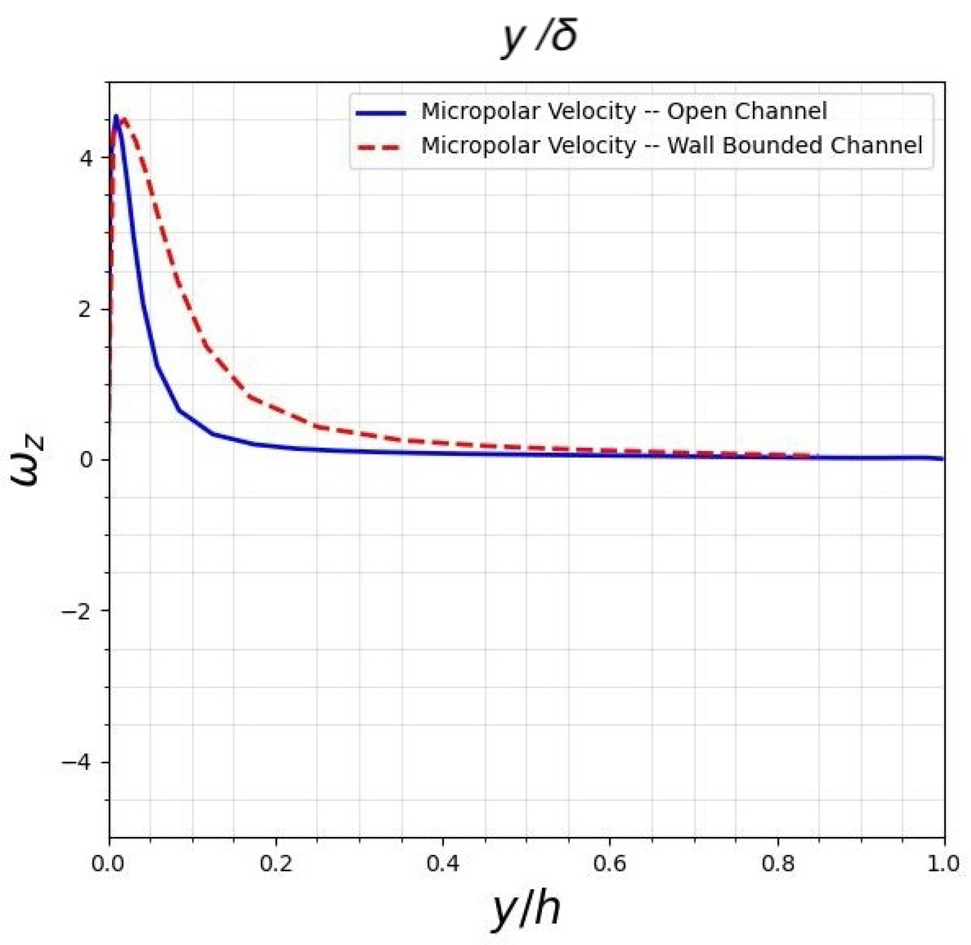
In order to examine the influence attenuation of the micropolar parameters in the open-channel flow case, the spanwise micropolar velocity profile along the channel total height (y/h) is plotted in Figure 5 and is compared against the respective spanwise micropolar velocity profile of the wall-bounded channel case. The wall-bounded channel case micropolar velocity profile is plotted along the characteristic length $\delta$ ($\delta =h/2$). The reason for that is that $\delta$ and h are both characteristic boundary layer thicknesses of the respective flows. Only the spanwise direction is presented for the micropolar velocity as it is the only direction in which micropolar velocity survives [14]. It is observed that the micropolar velocity presents peak values in both cases near the bottom wall ($y<0.3$). Additionally, by examining Figure 5 it is evident that the micropolar velocity profile in the current open-channel flow case drops very quickly to zero and has no influence after $y/h>0.1$. On the contrary, the micropolar velocity in the closed channel case “survives" at least up to $y/\delta \approx 0.3$. This observation further enhances our previous discussion about the influence attenuation of the micropolar parameters in the open-channel flow case.

Further evidence of the secondary phase presenting a strong influence only close to the bottom wall has been provided in previous experimental studies [2,23,24,25,26,27]. In these experiments, the particle velocity was measured as higher than the respective fluid phase one very close to the bottom wall.

3.2. Diagnostic Functions

To answer the question of whether a logarithmic layer exists in some interval of the mean velocity profile (MVP), which has been examined in Section 3.1, we calculate a diagnostic function defined as:

$$\Xi \left(y^{+}\right)=y^{+}{\displaystyle \frac{d{u}^{+}}{d{y}^{+}}}$$

(4)

If a logarithmic layer exists, then $\Xi =const.=1/\kappa$, where $\kappa$ is the von Kármán constant. In Figure 6, we graphically compare the distributions of ($\Xi$) for $m=0.0$ and $m=0.9$. Close to the channel bottom, $y^{+}\le 85$ ($y/h\le 0.25$), the two curves are indistinguishable on the scale of the graph. Thus, the effect of parameter m is negligible in the inner region of the turbulent boundary layer. A clear formation of a logarithmic layer is not observed for the $Re$ of this study. However, an upper bound of a “Kármán-like” constant can be estimated. Since it is found that ${\Xi }_{min}=2.46$, it is speculated that in a logarithmic layer at a higher Reynolds number the value of $\kappa$ will, most probably, be lower than $0.407(\approx 0.41)$.

Close to the free surface, $y^{+}\ge 138$ ($y/h\ge 0.42$), the two ($\Xi$) curves diverge. The curve for the case of $m=0.0$ forms an outer peak at $y^{+}\approx 180(y/h\approx 0.53)$. In contrast, the curve of case $m=0.9$ forms a plateau in the interval $0.4\le y/h\le 0.53$ corresponding to the logarithmic behavior of the form ${\displaystyle \frac{1}{{\kappa }_2}}ln{y}^{+}+G$ where ${\kappa }_2\approx 0.351$ (${\Xi }_{mean}=2.85$). This behavior can be marked as a characteristic of the outer layer in the micropolar turbulent case, due to the higher turbulent phenomena that are present in this case.

Next, we investigate the possibility of power law behavior in an interval of the (MVP). Here, we present the behavior of the diagnostic function $\Gamma ={\displaystyle \frac{y^{+}}{u^{+}}}{\displaystyle \frac{d{u}^{+}}{d{y}^{+}}}$. If a power law ($u^{+}=A{\left(y^{+}\right)}^{\lambda }$ ) with a constant exponent describes a “part” of the (MVP), then in that interval $\Gamma$ attains a constant value equal to $\lambda$. In Figure 7, the behavior of $\Gamma$ is presented for the cases of $m=0.0$ and $m=0.9$.

As expected, by examining $\Gamma$ function graphs it is confirmed that the effect of parameter (m) is negligible up to $y^{+}\le 125(y/h\le 0.38)$. An interval where $\Gamma$ function is approximately constant is observed at $60\le y^{+}\le 140(0.18\le y/h\le 0.42)$. This observation suggests that a power-law approximation of the (MVP), with an exponent of $\lambda \approx 0.162$, is satisfactory in this interval for both cases of $m=0$ and $m=0.9$. It is stressed here that these tentative conclusions concern the rather low turbulent Reynolds number case of $R{e}_b$ = 11,200.

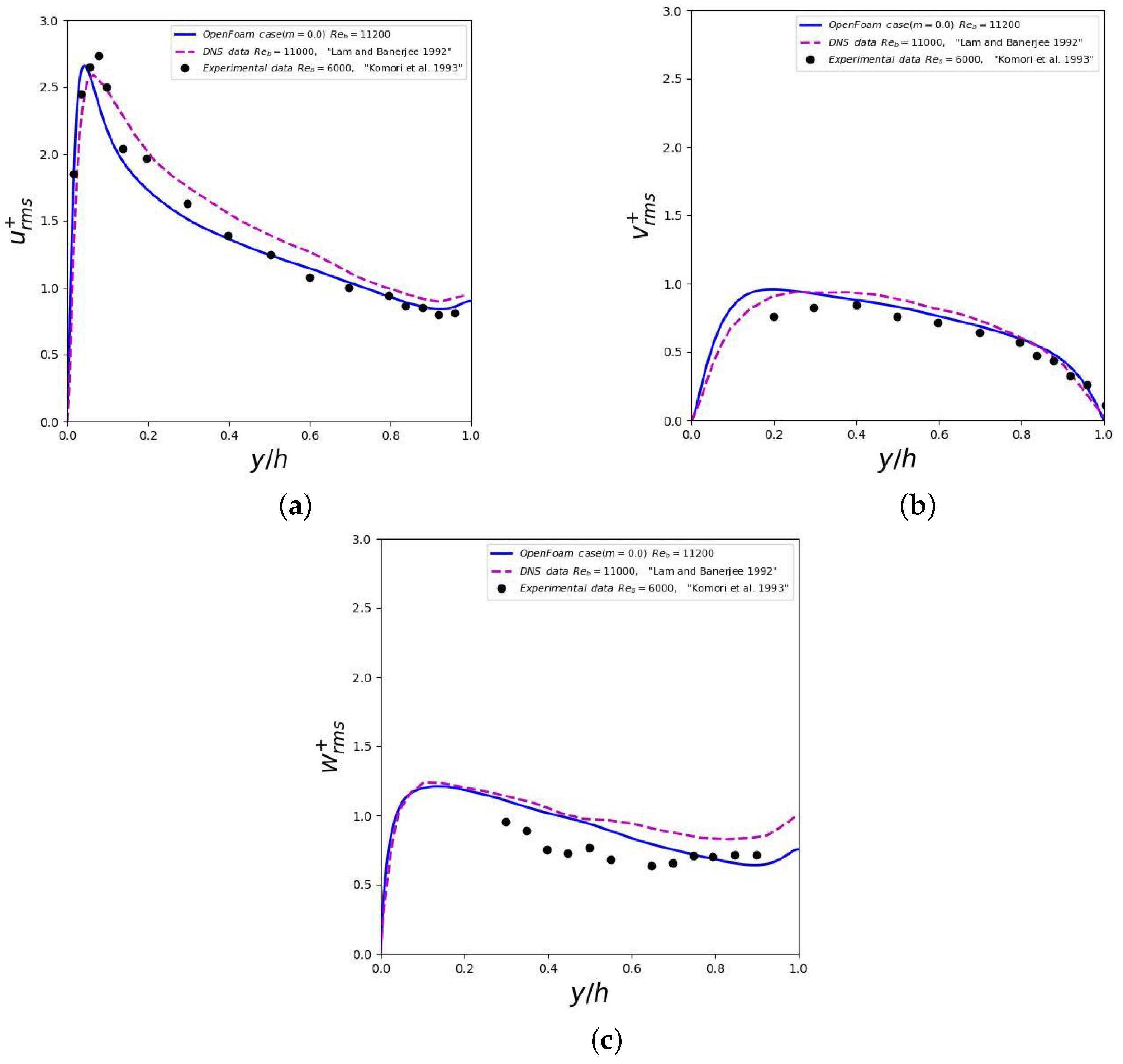
3.3. Turbulence Intensity

In order to further validate our present DNS code in the specific case of the open-channel geometry, the turbulence statistics have been analyzed and compared against the usual hydrodynamic case of computational and experimental studies. Turbulence intensity has been examined through root mean square (rms) velocity profiles, which have been normalized with the shear velocity $u_{\tau }$ and plotted against the wall distance normalized with the channel height, $y/h$. All three rms velocity components have been plotted and are presented in Figure 8a–c, compared with the results of Komori et al. [18] and Lam and Banerjee [19].

The convergence with both the experimental and previous DNS data is satisfactory. Moreover, in some cases the present DNS data have achieved a better fit with the experimental ones, compared to literature data. More specifically, the maximum local error between the present results and previous experimental ones varies from 13 to $25\%$ in Figure 8a–c. The turbulence intensity is accurately represented in all three components, while the peak of every case can be found close to the bottom wall. This phenomenon is more pronounced for the streamwise rms velocity profile ($u_{rms}^{+}$), as shown in Figure 8a. The peak of the $u_{rms}^{+}$ curve can be found in the area of $y/h<0.2$ (near wall region), while for $0.2<y/h<1.0$, the turbulence intensity drops sharply to lower values. An additional interesting phenomenon is that the present DNS data follow the trend of the experimental ones [18], for all velocity components, closer than previous DNS data [19]. Apart from the validation of our code in terms of the mean velocity profile, this result could add to its robustness as well.

Another point of investigation concerns the rms velocity profiles of the hydrodynamic case ($m=0$), which are compared to the micropolar case of $m=0.9$. Once again, the comparison is made against the “highest" micropolar case, in order for the differences to be more evident. The comparative analysis for the rms velocity between hydrodynamic and micropolar cases is presented in Figure 9a–c. Apart from the rms velocity profile curves of each case, the difference between these curves is plotted as well, as a shaded area, red, or blue, indicating the negative or positive difference between the hydrodynamic and micropolar case, respectively. The final difference values plotted have been normalized with the shear velocity so that, if the difference has a value of, for example, $0.5$, it will be equal to $u_{\tau }/2$.

The comparative analysis presented in Figure 9a–c is particularly important as it presents different trends for the rms velocity profiles in the three directions. In the streamwise direction, the Figure 9a turbulence intensity of the micrpolar case seems to have the same behavior as the respective case shown for the streamwise velocity profile. In this sense, the micropolar turbulence intensity exceeds that of the hydrodynamic case in the inner region, while it drops to lower values in the outer region. This is an expected observation as changes in turbulence intensity are connected to the changes in the velocity profile as well. Moreover, this result could be an indication of turbulent drag reduction in the outer region.

On the contrary, in the wall-normal and spanwise directions, there seems to be a constant lag between the hydrodynamic and micropolar case along the channel height. Similar trends for the turbulence intensity profiles have been also reported in previous studies [4,23,24]. In their study, Taniere et al. [23] have found that the streamwise rms velocity profile of the particles exceeds the one of the single-phase flow very close to the wall, while the opposite trend is observed in the outer region. Interestingly, in the wall-normal direction, the rms velocity profiles of particles present a constant lag compared to that of the carrier phase, which the authors attribute to the effects of inertia and gravity in this direction. The same observations have been noted by Kiger and Pan [24] as well, who commented that flow turbulence intensity exceeds the respective unladen one only in the streamwise direction and only in the area of $y^{+}<30$. Finally, the constant lag of the laden flow in the transverse direction has been clearly shown in the results of Kulick et al. [4].

3.4. Shear Stresses

The shear stress profile is presented for the same $R{e}_b$ = 11,200 as previous results of this study and compared once again with DNS and experimental data in Figure 10, for the hydrodynamic case ($m=0$). The shear stress is computed as:

$${\tau }_s=\overline{-\left(u^{\prime }{v}^{\prime }\right)}$$

(5)

where the overbar in Equation (5) denotes spatio-temporal averaged values. The shear stress profiles in Figure 10 have been appropriately normalized with the wall shear velocity $u_{\tau }$. The agreement between the present and previous DNS results is satisfying, with slight differences occurring in the near-wall region. The experimental results of Komori et al. [18] seem to reach in a peak value lower than the present and previous DNS results [19]. The maximum local error between present and previous experimental results seems to be ≈27%. This deviation in the shear stress peak value was also reported in the original study of Komori et al. [18], where they compared their experimental results with those of Kim et al. [28] and Lam and Banerjee [19], but they did not comment further on the source of this deviation.

Moreover, the shear stresses of the micropolar ($m=0.9$) and hydrodynamic ($m=0.0$) cases have been plotted in Figure 11 along with their difference normalized by $u_{\tau }$. The normalization of their difference follows the same approach as in the previous plots of velocity and turbulence intensity profiles. Upon closer examination of Figure 11, a similar trend with the streamwise velocity profile can be observed. This includes higher values of shear stress for the micropolar flow in the region ($y/h<0.5$), while the hydrodynamic flow reaches higher values in the region ($y/h>0.5$), indicating drag reduction phenomena in this region once again. These results are consistent with the findings in Figure 4, where the micropolar flow is faster than the hydrodynamic one in the region ($y/h<0.5$) and slower when ($y/h>0.5$) [12]. The only discrepancy in this trend occurs very close to the wall ($y/h<0.05$), where the hydrodynamic values exceed the micropolar ones, but this result may be connected to computational error, which may be observed in regions close to the wall.

The shear stress comparison between the single- and two-phase flow presented by Kiger and Pan [24] has revealed an opposite trend to the present results, without the authors really commenting on this behavior. In this instance, differences in every case are only marginal but still pose a clear behavior of each phase. Shear stress behavior in the present study has been also discussed in Muste et al. [26]. They have also reported a linear increment of the two-phase flow shear stress towards the bed, while the single flow shear stress has been constantly collapsing to higher values across the outer region. In addition, they have reported that previous studies present mixed behaviors as far as the shear stress is concerned. There are various studies that found no difference in the shear stress values between particulate and unladen flows, such as those of Best et al. [29] and Graf and Cellino [30]. On the other hand, the experimental work of Kaftori et al. [31] has found no change in the near-wall values but instead a decrease in the outer region for the shear stress values of the particulate flow.

4. Conclusions

In the present paper, an Eulerian approach based on the micropolar model [13] has been employed in order to study a turbulent particulate open-channel flow, at a relatively low Reynolds number. This type of flow is of particular interest for environmental and geological applications. The micropolar model seems to be an accurate alternative for the investigation of turbulent wall-bounded flows as it can treat a particulate flow in an Eulerian frame with reduced mathematical complications and computational cost. The characteristics of the secondary phase have been introduced in the governing equations through terms that represent the spin gradient, particle viscosity, and microinertia.

The unladen flow has been successfully validated against previous experimental [18] and computational [19] results. Next, cases of varying micropolar viscosity, which correspond to varying secondary phase characteristics, have been compared against the hydrodynamic one. Differences regarding the velocity distribution between the various micropolar cases are marginal. Therefore, the case of micropolar viscosity ratio $m=0.9$ has been compared against the hydrodynamic one, throughout the rest of the results section. One of the main disagreements in previous studies concerned the particle effect on the velocity distribution in an open-channel flow. The findings of the present study confirm the suggestions of Yu et al. [12] that the velocity distribution of the particulate flow presents mixed behavior compared to the unladen one. More specifically, it has been shown here that the velocity values of the particulate flow exceed the respective unladen ones in the inner region, while they collapse to lower values in the outer region. This may be attributed to the particles’ trend of being accelerated by turbulent structures in the near-wall region.

The flow phenomena have been further examined through turbulence intensity plots. In the streamwise direction, the same trend between the particulate and single-phase flow has been observed, as in the mean velocity distribution. On the contrary, in the two other directions of the turbulence intensity, a constant lag between the two cases seems to exist, with the single-flow phase presenting slightly higher values of the order of $u_{\tau }/2$. Furthermore, the Reynolds shear stress profile has been plotted for the micropolar and hydrodynamic cases. The expected mixed behavior in the inner and outer regions of the flow has been confirmed. Previous studies presented controversial results, without really commenting on their observations.

To sum up, the micropolar model has shown various advantages over existing Lagrangian models when studying particulate flows, in terms of reduced computational cost and modeling complexity. Here, we have verified that this is an accurate and reliable method to analyze basic turbulent flow cases, usually found in environmental flows. Future studies should exploit the incorporation of the micropolar model in the analysis of more complex environmental and geological flows. Further DNS simulations are required for the development of composite mean velocity profile mathematical models [32], as well as accurate turbulence models very close to the wall [33].

References

1. Rashidi, M.; Hetsroni, G.; Banerjee, S. Particle-turbulence interaction in a boundary layer. Int. J. Multiph. Flow 1990, 16, 935–949. [Google Scholar] [CrossRef]
2. Kaftori, D.; Hetsroni, G.; Banerjee, S. Particle behavior in the turbulent boundary layer. II. Velocity and distribution profiles. Phys. Fluids 1995, 7, 1107–1121. [Google Scholar] [CrossRef]
3. Nezu, I.; Azuma, R. Turbulence characteristics and interaction between particles and fluid in particle-laden open-channel flows. J. Hydraul. Eng. 2004, 130, 988–1001. [Google Scholar] [CrossRef]
4. Kulick, J.D.; Fessler, J.R.; Eaton, J.K. Particle response and turbulence modification in fully developed channel flow. J. Fluid Mech. 1994, 277, 109–134. [Google Scholar] [CrossRef]
5. Crowe, C.; Troutt, T.; Chung, J. Numerical models for two-phase turbulent flows. Annu. Rev. Fluid Mech. 1996, 28, 11–43. [Google Scholar] [CrossRef]
6. Dritselis, C.D.; Vlachos, N.S. Numerical study of educed coherent structures in the near-wall region of a particle-laden channel flow. Phys. Fluids 2008, 20, 055103. [Google Scholar] [CrossRef]
7. Balachandar, S.; Eaton, J.K. Turbulent dispersed multiphase flow. Annu. Rev. Fluid Mech. 2010, 42, 111–133. [Google Scholar] [CrossRef]
8. Kidanemariam, A.G.; Chan-Braun, C.; Doychev, T.; Uhlmann, M. Direct numerical simulation of horizontal open-channel flow with finite-size, heavy particles at low solid volume fraction. New J. Phys. 2013, 15, 025031. [Google Scholar] [CrossRef]
9. Gao, W.; Samtaney, R.; Richter, D.H. Direct numerical simulation of particle-laden flow in an open channel at. J. Fluid Mech. 2023, 957, A3. [Google Scholar] [CrossRef]
10. Rouson, D.W.; Eaton, J.K. On the preferential concentration of solid particles in turbulent channel flow. J. Fluid Mech. 2001, 428, 149–169. [Google Scholar] [CrossRef]
11. Bernardini, M.; Pirozzoli, S.; Orlandi, P. The effect of large-scale turbulent structures on particle dispersion in wall-bounded flows. Int. J. Multiph. Flow 2013, 51, 55–64. [Google Scholar] [CrossRef]
12. Yu, K.; Yoon, B.; Kim, D. Re-evaluation of change of mean velocity profiles in turbulent open-channel flows due to introducing sediment particles. KSCE J. Civil Eng. 2014, 18, 2261–2267. [Google Scholar] [CrossRef]
13. Eringen, A.C. Theory of micropolar fluids. J. Math. Mech. 1966, 16, 1–18. [Google Scholar] [CrossRef]
14. Sofiadis, G.; Sarris, I. Microrotation viscosity effect on turbulent micropolar fluid channel flow. Phys. Fluids 2021, 33, 095126. [Google Scholar] [CrossRef]
15. Sofiadis, G.; Sarris, I. Reynolds number effect of the turbulent micropolar channel flow. Phys. Fluids 2022, 34, 075126. [Google Scholar] [CrossRef]
16. Bender, J.; Koschier, D.; Kugelstadt, T.; Weiler, M. A micropolar material model for turbulent SPH fluids. In Proceedings of the ACM SIGGRAPH, Eurographics Symposium on Computer Animation, Montreal, QC, Canada, 21–23 August 2017; pp. 1–8. [Google Scholar]
17. Wang, L.; Chu, X. An extended CFD-DEM model based on micropolar fluid and its application in geological engineering. Comput. Geotech. 2023, 154, 105133. [Google Scholar] [CrossRef]
18. Komori, S.; Nagaosa, R.; Murakami, Y.; Chiba, S.; Ishii, K.; Kuwahara, K. Direct numerical simulation of three-dimensional open-channel flow with zero-shear gas–liquid interface. Phys. Fluids A Fluid Dyn. 1993, 5, 115–125. [Google Scholar] [CrossRef]
19. Lam, K.; Banerjee, S. On the condition of streak formation in a bounded turbulent flow. Phys. Fluids A Fluid Dyn. 1992, 4, 306–320. [Google Scholar] [CrossRef]
20. Bauer, C.; Sakai, Y.; Uhlmann, M. Direct numerical simulation of turbulent open-channel flow: Streamwise turbulence intensity scaling and its relation to large-scale coherent motions. In Proceedings of the 10th International Conference on Turbulence, Rome, Italy, 11–15 September 2023. [Google Scholar]
21. Coleman, N.L. Velocity profiles with suspended sediment. J. Hydraul. Res. 1981, 19, 211–229. [Google Scholar] [CrossRef]
22. Vanoni, V.A.; Nomicos, G.N. Resistance properties of sediment-laden streams. Trans. Am. Soc. Civil Eng. 1960, 125, 1140–1167. [Google Scholar] [CrossRef]
23. Taniere, A.; Oesterle, B.; Monnier, J. On the behaviour of solid particles in a horizontal boundary layer with turbulence and saltation effects. Exp. Fluids 1997, 23, 463–471. [Google Scholar] [CrossRef]
24. Kiger, K.; Pan, C. Suspension and turbulence modification effects of solid particulates on a horizontal turbulent channel flow. J. Turbul. 2002, 3, 019. [Google Scholar] [CrossRef]
25. Righetti, M.; Romano, G.P. Particle–fluid interactions in a plane near-wall turbulent flow. J. Fluid Mech. 2004, 505, 93–121. [Google Scholar] [CrossRef]
26. Muste, M.; Yu, K.; Fujita, I.; Ettema, R. Two-phase flow insights into open-channel flows with suspended particles of different densities. Environ. Fluid Mech. 2009, 9, 161–186. [Google Scholar] [CrossRef]
27. Noguchi, K.; Nezu, I. Particle–turbulence interaction and local particle concentration in sediment-laden open-channel flows. J. Hydro-Environ. Res. 2009, 3, 54–68. [Google Scholar] [CrossRef]
28. Kim, J.; Moin, P.; Moser, R. Turbulence statistics in fully developed channel flow at low Reynolds number. J. Fluid Mech. 1987, 177, 133–166. [Google Scholar] [CrossRef]
29. Best, J.; Bennett, S.; Bridge, J.; Leeder, M. Turbulence modulation and particle velocities over flat sand beds at low transport rates. J. Hydraul. Eng. 1997, 123, 1118–1129. [Google Scholar] [CrossRef]
30. Graf, W.; Cellino, M. Suspension flows in open channels; experimental study. J. Hydraul. Res. 2002, 40, 435–447. [Google Scholar] [CrossRef]
31. Kaftori, D.; Hetsroni, G.; Banerjee, S. The effect of particles on wall turbulence. Int. J. Multiph. Flow 1998, 24, 359–386. [Google Scholar] [CrossRef]
32. Liakopoulos, A. Explicit representations of the complete velocity profile in a turbulent boundary layer. AIAA J. 1984, 22, 844–846. [Google Scholar] [CrossRef]
33. Liakopoulos, A. Computation of high speed turbulent boundary-layer flows using the k– ϵ turbulence model. Int. J. Numer. Methods Fluids 1985, 5, 81–97. [Google Scholar] [CrossRef]
Figure 1. Schematic of the geometry that has been used in the present study, where h = 2 δ .
Fluids 09 00202 g001
Figure 2. Normalized mean velocity profile of the present hydrodynamic case compared against experimental results of Komori et al. [18] and DNS results of Lam and Banerjee [19] and of Bauer et al. [20].
Fluids 09 00202 g002
Figure 3. Normalized mean velocity profile of the present hydrodynamic case, compared against micropolar cases at the same R e b .
Fluids 09 00202 g003
Figure 4. Mean velocity profile of the present hydrodynamic case, compared against the micropolar case of m = 0.9 at the same R e b , in outer units.
Fluids 09 00202 g004
Figure 5. Mean spanwise micropolar velocity profile of the present open-channel case, compared against wall-bounded channel case at the same R e b = 11,200 and m = 0.4 . The open-channel case is normalized with the total channel height (h), while the closed channel case with ( δ = h / 2 ).
Fluids 09 00202 g005
Figure 6. Diagnostic function ( Ξ ) plots of the present DNS data, for R e b = 11,200 and cases of m = 0.0 and m = 0.9 , plotted in inner-law units.
Fluids 09 00202 g006
Figure 7. Power-law diagnostic function ( Γ ) based on the present DNS data, for R e b = 11,200 and cases of m = 0.0 and m = 0.9 , plotted in inner-law units.
Fluids 09 00202 g007
Figure 8. Normalized (a) u r m s , (b) v r m s , and (c) w r m s velocity profiles of the hydrodynamic case ( m = 0 ) plotted against global coordinates and compared with experimental results of Komori et al. [18] and DNS results of Lam and Banerjee [19].
Fluids 09 00202 g008
Figure 9. Normalized (a) u r m s , (b) v r m s , and (c) w r m s velocity profiles of the hydrodynamic case ( m = 0 ) compared with the micropolar case ( m = 0.9 ), plotted against global coordinates. The final difference values (shaded area) have been normalized with the shear velocity so that, if the difference has a value of, for example, 0.5 , it will be equal to u τ / 2 .
Fluids 09 00202 g009
Figure 10. Normalized shear stress profiles of the hydrodynamic case ( m = 0 ) R e b = 11,200, compared with experimental results of Komori et al. [18] and DNS results of Lam and Banerjee [19], plotted against normalized wall distance.
Fluids 09 00202 g010
Figure 11. Normalized shear stress profiles of the hydrodynamic case ( m = 0 ), compared with the micropolar case of ( m = 0.9 ), for R e b = 11,200, plotted against normalized wall distance. The shaded areas represent the difference between the two normalized stress profiles: (red shade) ( u v ) ¯ m = 0 < ( u v ) ¯ m = 0.9 , (blue shade) ( u v ) ¯ m = 0 > ( u v ) ¯ m = 0.9 .
Fluids 09 00202 g011