An Analysis of Water Leakages in Series Pipelines Using the Rigid Column Model

Abstract

Water leakages are assessed with an extended period simulation (traditional analysis) in water distribution networks. However, when rapid manoeuvres regulate valves, the conventional analysis proves unsuitable for representing the water volume of leaks. Under these circumstances, the Rigid Water Column Model can be utilised to accurately compute the quantity of water volume leaks. This method has been applied to single and parallel pipelines to predict water leakages, considering the opening and closure manoeuvres of regulating valves. This research develops governing equations using the Rigid Column Model to predict water volume leaks in a general scheme of series pipelines, accounting for the opening and closure manoeuvres in regulating valves. The practical application involves two branches of a series pipeline with internal pipe diameters of 0.45 and 0.25 m and pipe lengths of 1200 and 1400 m, respectively. The results of this practical application demonstrate the accuracy of the Rigid Column Model and its relevance in real-world scenarios. For instance, the model shows that traditional analysis can overestimate water volume leaks by approximately 72% when a closure manoeuvre regulates valves for 200 s and by about 28% for 30 s, highlighting the need for a more accurate method.

1. Introduction

Most mathematical models for computing water leakages [1] in water distribution networks rely on extended-period simulations, classified as non-inertial models [2]. These models consider dynamic effects by considering the variability in boundary conditions, making them suitable for prolonged transient events such as manoeuvres in regulating valves that last for hours [3]. Researchers and engineers have widely adopted EPANET software 2.2.0 [4,5] because it accurately simulates pressure-dependent (PDC) and pressure-independent (PIC) consumption [6]. PIC is characterised by delivering a constant flow rate regardless of pressure oscillations, while PDC has a different amount of water flow depending on pressure variations. EPANET software uses the extended period simulation to make calculations. The water balance methodology of the International Water Association (IWA) is commonly used to quantify all consumption in water distribution systems to determine the sources of water losses. In this sense, billed and unbilled authorised consumption and apparent and physical losses can be computed using this methodology [7,8]. A thorough analysis should identify the simulated input water volumes using PDC and those using PIC. Specifically, pipe water leakages are modelled using PIC, as higher-pressure heads in water supply systems correlate with increased water flow leakages [9,10]. Water leakages are more significant during nighttime than daytime [11], as pressure values are greater at night than during the day.

Recently, water utilities have encountered the challenge of developing robust models capable of virtually representing water distribution systems using artificial intelligence techniques to detect and predict water leakages, known as digital twins [11,12,13]. Implementing these models requires a dependable hydraulic layer of the water distribution systems. However, there needs to be more literature concerning the computation of pipe water leakages during short-term opening and closure manoeuvres of regulating valves, where non-inertial models cannot simulate these events accurately. In such cases, inertial models are necessary for an accurate virtual representation of hydraulic installations because they account for rapid changes that can occur, such as valve manoeuvres.

Inertial models can be divided into two groups: the Elastic Column Model (ECM) [14] and the Rigid Column Model (RCM) [15]. The ECM considers the elasticity of water and pipes, whereas the RCM neglects them. They have been employed to compute hydraulic transient events, analysing variations in pressure head pulses during rapid manoeuvres of regulating valves and pump stoppages [16,17]. According to previous publications by the authors, the ECM and RCM yield comparable results because leaks relieve pressure heads by expelling a specific quantity of water flow. The authors have developed a mathematical model to analyse pipe water leakages in single and parallel systems [18,19]. The model integrates the RCM [18] and a continuity equation incorporating IWA’s water balance principles [20]. This approach is crucial because it considers the system’s inertia, which becomes significant during rapid variations caused by regulating valves’ opening and closure manoeuvres. This combined model enables a more accurate representation of hydraulic dynamics, especially for rapid changes within water distribution networks.

This paper presents a theoretical model and demonstrates its practical application involving two branches of pipes. The main hydraulic variables—pressure head, water flow in pipes, and friction factor—are computed for each pipe, providing a comprehensive understanding of the system’s behaviour. By performing both opening and closure manoeuvres, the total volume of leaks under these conditions is calculated, and a comparison with the extended period simulation (traditional model) is conducted to highlight the practical implications of neglecting the system’s inertia.

This research significantly contributes to the existing literature by introducing a novel mathematical model for analysing water leakages in series pipelines during rapid valve opening and closure manoeuvres. Based on the RCM, the proposed model presents a general framework that can be applied to series pipelines with any number of branches, thereby expanding the scope of research in this area.

2. Mathematical Model

This section presents a general framework for analysing water leakages in series pipelines, considering the effects of regulating valves, often overlooked by traditional methods (extended period simulation). The hydraulic system is divided into $n$ pipe branches, as illustrated in Figure 1. Given the series pipeline configuration, the number of consumption nodes corresponds to the number of pipe branches. The initial pressure, denoted by the notation $z_0$, is supplied by either a reservoir or a pumping station. The subscript $i$ refers to a specific pipe branch or consumption node. The subscript $n$ is the total pipe branches in a hydraulic system.

The system comprises $Q_i$ consumption nodes, and each pipe branch is characterised by an internal diameter $d_i$, a length $l_i$, and an absolute roughness of the pipe surface $k_{s,i}$. Each node has an elevation $z_i$ and a pressure head $p_i/{\gamma }_w$. Pipe branch $i$ transports a water flow $q_i$ and may generate a water leakage $Q_{li}$. Traditional methods are inadequate for simulating valve manoeuvres where the variation in the resistance coefficient $R_{vi}$ is neglected over time. It depends on the valve manoeuvre and its operation mode (manual or automatic). It represents the opening position as a function of the opening degree.

The proposed model addresses this effect by employing an inertial model, where the water phase’s elasticity and the pipe thickness deformations are neglected (RCM).

2.1. Assumptions

The assumptions of the proposed model are described as follows:

• The Rigid Column Model describes water movement within pipelines, focusing on dynamics influenced by valve operations and hydraulic conditions. The elasticity of the water and pipe can be neglected since water leakages tend to relieve the pressure, making the RCM applicable.
• Steady friction is assumed and is employed to compute longitudinal energy losses generated by pipes.
• Pipe branches have a constant internal diameter and absolute roughness.
• The fluid is assumed to be represented by a single streamline, and velocity distribution is lumped into average distribution.
• The pressure distribution is only considered along pipes.
• Water leaks are located downstream of regulating valves.
• The continuity equation is applied considering the terms of the different levels for the water balance proposed by the IWA (see

  Table 1. The main water balance components proposed by the IWA.

  Level 1	Level 2	Level 3	Level 4
  Input water volume	Authorised Consumption	Billed Authorised Consumption	Domestic Consumption ($Q_{DC}$) Industrial Consumption ($Q_{IC}$) Official Consumption ($Q_{OC}$) Commercial Consumption ($Q_{CC}$)
  		Unbilled Authorised Consumption
  	Water Losses	Apparent Losses
  		Real Losses (physical losses)	Pipe water leakages ($Q_l$) Other water leakages

  ).

2.2. Governing Equations

Based on the assumptions, the governing equations of the proposed model are as follows:

1.

The mass oscillation equation.

This formulation can represent the water movement to a pipe branch. The authors previously developed and demonstrated this equation in the context of single pipelines [18]. For series pipelines, the equation is given by:

$${\displaystyle \frac{d{q}_i}{dt}}={\displaystyle \frac{\left[z_{i-1}+\raisebox{1ex}{$p_{i-1}$}\!\left/ \!\raisebox{-1ex}{${\gamma }_w$}\right.-z_i-\raisebox{1ex}{$p_i$}\!\left/ \!\raisebox{-1ex}{${\gamma }_w$}\right.\right]g\pi d_i^2}{4l_i}}-{\displaystyle \frac{2f_i{q}_i\left|q_i\right|}{\pi d_i^3}}-{\displaystyle \frac{R_{v,i}{q}_i\left|q_i\right|g\pi d_i^2}{4l_i}}-{\displaystyle \frac{2\sum k_{m,i}{q}_i\left|q_i\right|}{\pi l_i{d}_i^2}}$$

(1)

where $z_{i-1}$ = elevation in node $i-1$, $z_i$ = elevation in node $i$, $p_i/{\gamma }_w$ = pressure head in node $i$, $p_{i-1}/{\gamma }_w$ = pressure head in node $i-1$, ${\gamma }_w$ = water unit weight, $f_i$ = friction factor for pipe $i$, $q_i$ = water flow passing for pipe $i$, $d_i$ = pipe diameter for pipe $i$, $l$ = pipe length $i$, $\sum k_m$ = minor losses global coefficient in pipe $i$, $R_v$ = resistance coefficient of regulating valve located at pipe $i$, and $g$ = gravitational acceleration constant.

2.

The continuity equation.

Applying the continuity equation requires a detailed analysis of the water balance. In this sense, the IWA’s water balance, presented in Table 1, was considered for this study. The total input water volume is divided into authorised consumption and water losses. For modelling purposes, the billed authorised consumption can be computed as the sum of domestic ($Q_{DC}$), industrial ($Q_{IC}$), official ($Q_{OC}$), and commercial ($Q_{CC}$) consumptions. For the development of the proposed model, pipe water leakages are represented as $Q_l$. The proposed model can also include unbilled authorised consumption, apparent losses, and other water leakages.

Considering Figure 1 and the terms in

Table 2. Computation of water volume of leakages.

Time Analysed (s)		Total Volume of Water Leakages (m3)
From	To	Extended Period Simulation	Proposed Model
			Opening Manoeuvre	Closure Manoeuvre
0	30	4.35	2.40	3.25
0	200	28.98	27.14	8.12

, the continuity equation can be expressed as:

$$q_i=\sum _{i=1}^n\left(Q_{DCi}+Q_{ICi}+Q_{OCi}+Q_{CCi}\right)+\sum _{i=1}^n{Q}_{li}$$

(2)

where $n$ = number of pipe branches.

The water flows $Q_{DCi}$, $Q_{ICi}$, $Q_{OCi}$, and $Q_{CCi}$ can be modelled using a pressure-independent consumption approach. These terms can be computed considering the expression $Q_C=C\overline{Q}$, where $Q_C$ = water flow variations for a billed authorised consumption, $C$ = modulation coefficient, and $\overline{Q_C}$ = average $Q_C$. Water utilities must establish modulation coefficients based on records from water distribution systems.

Pipe water leakages ($Q_l$) are estimated using a pressure-dependent consumption approach. Usually, water leakages are simulated using an emitter coefficient ($K_f$), which can be considered constant for a group of installed pipelines. This flow also depends on the pressure head computed in a node $i$. The exponent coefficient should be regarded as 0.5. Then, water leakages can be modelled using the expression $Q_{li}=K_f\sqrt{p_i/{\gamma }_w}$.

3.

The friction factor equation

The friction factor is dependent on the Reynolds number. In water distribution systems, most problems involve turbulent flow conditions. For calculation purposes, the Swamee–Jain equation [21,22] was employed to estimate the friction factor, as this explicit formulation consistently produces results with an accuracy rate of less than 1% error compared to the Colebrook–White formulation,

$$f_i={\displaystyle \frac{0.25}{{\left[\log \left(\frac{k_{s,i}}{3.7d_i}+\frac{5.74}{{\mathrm{R}\mathrm{e}}_i^{0.9}}\right)\right]}^2}}$$

(3)

where $k_s$ = absolute roughness and $\mathrm{R}\mathrm{e}$ = Reynolds number.

2.3. Boundary and Initial Conditions

The upstream boundary condition is defined by the value of $z_0$, representing the energy input from either a pumping station system or a reservoir. The downstream boundary condition is determined by atmospheric pressure.

The initial condition is established from the extended period simulation for two analysed scenarios (opening and closure operations). These results are influenced by the manoeuvres in regulating valves, as follows:

• For opening manoeuvres in regulating valves, the system is at rest, and water velocities are 0 m/s.
• For closure manoeuvres in regulating valves, the condition given during the extended-period simulation establishes the initial water velocity.

2.4. Numerical Resolution

The Simulink tool in MATLAB was employed to solve the system of algebraic differential equations represented by Equations (1)–(3) for each series branch. The total number of equations is $3n$. The unknown variables in this problem are $p_i/{\gamma }_w$, $q_i$, and $f_i$.

2.5. Methodology

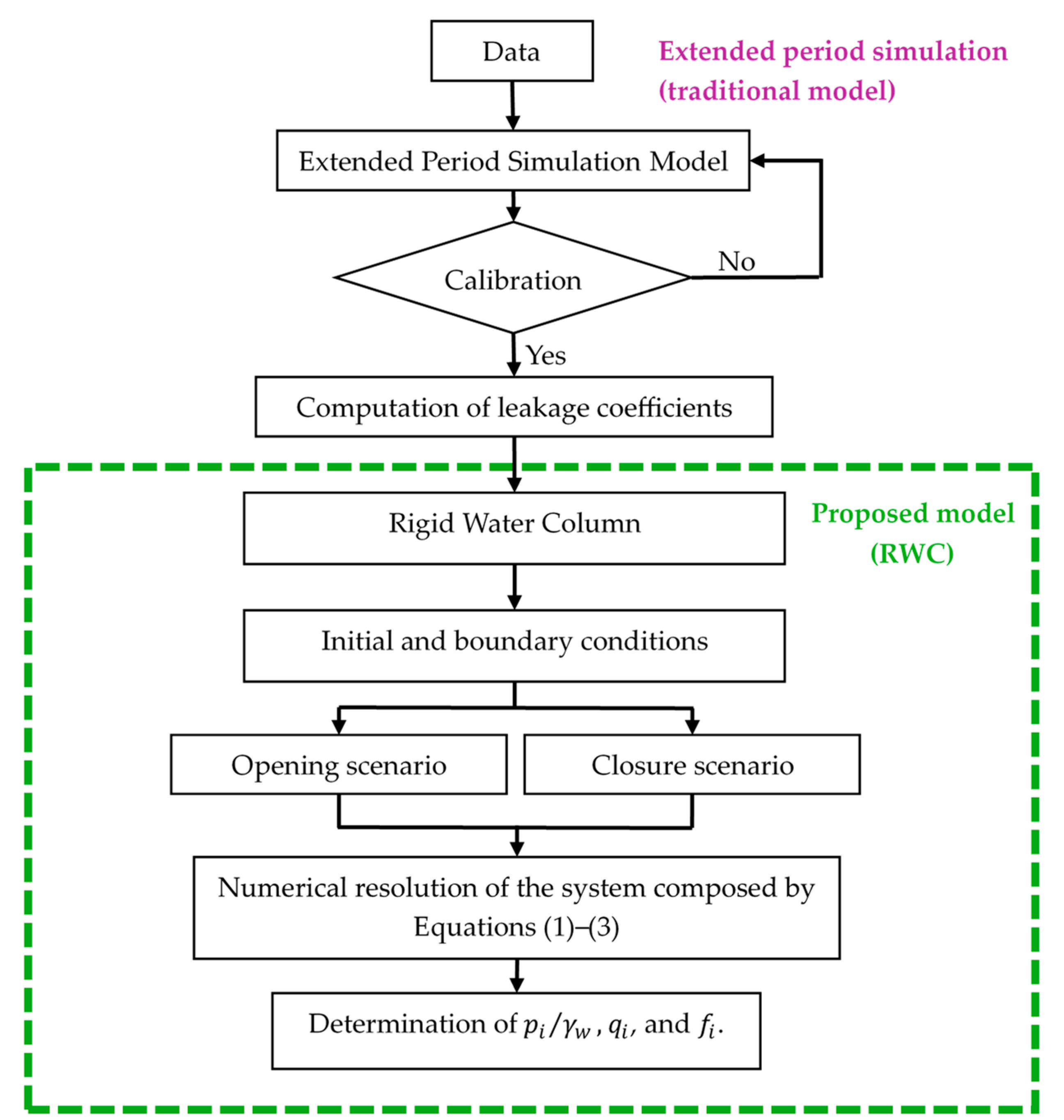
The traditional model focuses on considering an extended period simulation, which requires input data on base demands and modulation coefficients for domestic ($Q_{DC}$), industrial ($Q_{IC}$), official ($Q_{OC}$), and commercial ($Q_{CC}$) consumption. Pipe water leakages are calculated based on emitter coefficients. In all cases, prior calibration of emitter coefficients ($K_f$) is necessary to accurately compute water leakages in pipes during the extended period simulation.

In this research, the procedure for applying the proposed model is also presented in Figure 2. Considering the results of the extended period simulation (traditional model), the Rigid Column Model requires defining the initial and boundary conditions (see Section 2.3). Since the conventional model is unsuitable for computing water leakages when regulating valves are active, the proposed model addresses this issue by considering the system inertia. It is of utmost importance to have an understanding of valve manoeuvres over time. Finally, the numerical resolution composed of Equations (1)–(3) is solved using Simulink of MATLAB R2021b, employing the ODE23s (stiff/Mod. Rosenbrock) solver with a relative tolerance of $1·{10}^{-3}$.

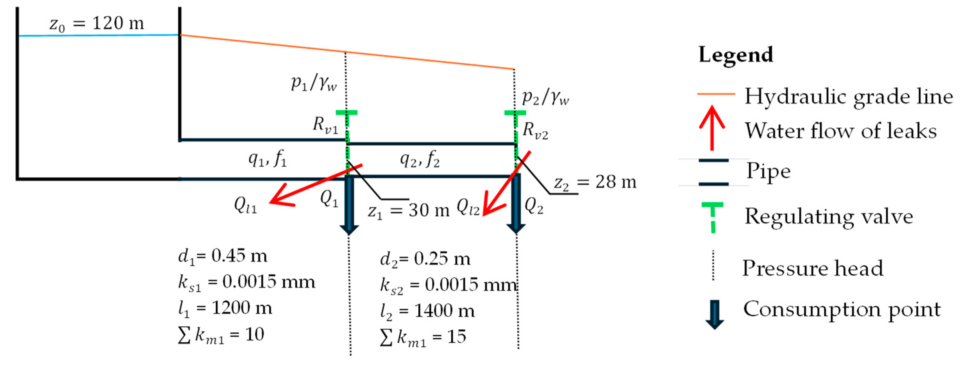
3. Practical Application for Series Pipelines

The case study analysed in this research corresponds to a series of pipelines composed of two branches ($n=2$). The data of the pipes are: $d_1$ = 0.45 m, $d_2$ = 0.25 m, $l_1$ = 1200 m, $l_2$ = 1400 m, $k_{s1}$ = $k_{s2}$ = 0.0015 mm, $\sum k_{m1}$ = 10, and $\sum k_{m1}$ = 15. The initial water level ($z_0$) is 120 m, supplied by a reservoir. The elevation points of pipes are $z_1$ = 30 m and $z_2$ = 28 m. Figure 3 presents data for the practical application. A kinematic viscosity of $1·{10}^{-6}$ m²/s was used. Nodes 1 and 2 are located at the end of pipe branches 1 and 2, respectively, as shown in Figure 3.

In this practical application, only domestic and industrial consumptions were considered using average values of $\overline{Q_{DC1}}$ = 78.9 L/s, $\overline{Q_{DC2}}$ = 68.4 L/s, $\overline{Q_{IC1}}$ = 17.5 L/s, and $\overline{Q_{IC2}}$ = 12.6 L/s. For this problem, the daily modulation coefficients are presented in Figure 4, considering that nodes 1 and 2 have the same domestic consumption patterns. The extreme modulation coefficients for domestic consumption are 0.4 and 1.6. For industrial consumption, the maximum values at nodes 1 and 2 are 1.8 and 1.9, respectively, while the minimum values are 0.2 in both nodes.

Based on the results of the traditional model’s application, the emitter coefficients of $K_{f1}$ = 0.00925 and $K_{f2}$ = 0.0085 m³/s/m^0.5 were obtained using the extended period simulation. The proposed model requires starting with the definition of these coefficients, which can be calibrated using previously developed methodologies [10,20].

The scenarios of opening and closing manoeuvres in regulating valves have been modelled over 30 s, using resistance coefficients of 210 ms²/m⁶ for $R_{v1}$ and 250 ms²/m⁶ for $R_{v2}$, respectively.

The governing equations of this problem are presented as follows:

a.

Continuity equation for pipe 1

$$p_1/{\gamma }_w={\left({\displaystyle \frac{q_1-q_2-C_{DC1}\overline{Q_{DC1}}-C_{IC1}\overline{Q_{IC1}}}{K_{f1}}}\right)}^2$$

(4)

b.

Momentum equation for pipe 1 (between nodes 0 and 1)

$${\displaystyle \frac{d{q}_1}{dt}}={\displaystyle \frac{\left[z_0-z_1-\raisebox{1ex}{$p_1$}\!\left/ \!\raisebox{-1ex}{${\gamma }_w$}\right.\right]g\pi d_1^2}{4l_1}}-{\displaystyle \frac{2f_1{q}_1\left|q_1\right|}{\pi d_1^3}}-{\displaystyle \frac{R_{v,1}{q}_1\left|q_1\right|g\pi d_1^2}{4l_1}}-{\displaystyle \frac{2\sum k_{m,1}{q}_1\left|q_1\right|}{\pi l_1{d}_1^2}}$$

(5)

In Equation (5), the term $z_0$ corresponds to the total piezometric head in the reservoir.

c.

Friction factor equation for pipe 1

$$f_1={\displaystyle \frac{0.25}{{\left[\log \left(\frac{k_{s,1}}{3.7d_1}+\frac{5.74}{{\mathrm{R}\mathrm{e}}_1^{0.9}}\right)\right]}^2}}$$

(6)

d.

Continuity equation for pipe 2

$$p_2/{\gamma }_w={\left({\displaystyle \frac{q_1-C_{DC1}\overline{Q_{DC1}}-C_{DC2}\overline{Q_{DC2}}-C_{IC1}\overline{Q_{IC1}}-C_{IC2}\overline{Q_{IC2}}-K_{f1}\sqrt{p_1/{\gamma }_w}}{K_{f2}}}\right)}^2$$

(7)

e.

Momentum equation for pipe 2 (between nodes 1 and 2)

$${\displaystyle \frac{d{q}_2}{dt}}={\displaystyle \frac{\left[z_1+\raisebox{1ex}{$p_1$}\!\left/ \!\raisebox{-1ex}{${\gamma }_w$}\right.-z_2-\raisebox{1ex}{$p_2$}\!\left/ \!\raisebox{-1ex}{${\gamma }_w$}\right.\right]g\pi d_2^2}{4l_2}}-{\displaystyle \frac{2f_2{q}_2\left|q_2\right|}{\pi d_2^3}}-{\displaystyle \frac{R_{v,2}{q}_2\left|q_2\right|g\pi d_2^2}{4l_2}}-{\displaystyle \frac{2\sum k_{m,2}{q}_2\left|q_2\right|}{\pi l_2{d}_2^2}}$$

(8)

f.

Friction factor equation for pipe 2

$$f_2={\displaystyle \frac{0.25}{{\left[\log \left(\frac{k_{s,2}}{3.7d_2}+\frac{5.74}{{\mathrm{R}\mathrm{e}}_2^{0.9}}\right)\right]}^2}}$$

(9)

Equations (4) and (7) were obtained by organising terms in Equation (2).

The numerical resolution of Equations (4) to (9) provides the responses for the six unknown variables: $p_1/{\gamma }_w$, $p_2/{\gamma }_w$, $q_1$, $q_2$, $f_1$, and $f_2$.

4. Results

4.1. Extended Period Simulation

The extended period simulation lasted an entire day (86,400 s) and tracked the progression of water flow leaks in the practical application (Section 3). The initial conditions are given by $q_1\left(0\right)$ = 211.87 and $q_2 \left(0\right)$ = 95.37 L/s. Figure 5 illustrates the patterns of the pressure head, total water flow, and water flow leaks. In Figure 5a, the pressure head initiates at 120 wcm (Point 0); however, friction losses gradually decrease the hydraulic grade line values, as indicated by Points 1 and 2. The pressure head reaches its minimum values of 50.78 wcm (at 43,010 s) and 7.73 wcm (at 43,278 s) for Points 1 and 2, respectively. Regarding the total water flow patterns in Pipe 1, two peak flow rates are reached at 366.23 and 350.49 L/s, occurring at 43,294 and 61,532 s, respectively, as depicted in Figure 5b. Pipe 1 exhibits the highest water flow compared to the values observed in Pipe 2. Figure 5c shows the water flow leaks for Pipes 1 and 2, where water leakages in Pipe 1 are higher than in Pipe 2 since greater pressure head values are reached at Node 1.

4.2. Proposed Model

The proposed model was run considering the two scenarios of closure and opening manoeuvres of regulating valves. Figure 6 presents the results under the closure manoeuvre consideration for the first 200 s, with the closure manoeuvre completed in 30 s. The initial conditions are the same as those of the extended period simulation.

Figure 6a shows the variation in the pressure head. The pressure head at Point 0 ($z_0$) remains constant throughout the transient event, with a value of 120 wcm. Due to the closure manoeuvre, the pressure head decreases at Points 1 and 2, reaching minimum values of 7.36 and 0.01 wcm, respectively. The water flow pulses also decrease, reaching minimum values of 94.33 and 31.08 L/s, as shown in Figure 6b.

Considering the water flow passing through the pipes, the friction factor varies from 0.0127 to 0.0147 and from 0.0132 to 0.0163 for Pipes 1 and 2, respectively. The water flow leaks are related to the pressure head in each node (point). The minimum values of water flow leaks are 25.1 and 0.82 L/s for Pipes 1 and 2, respectively, as depicted in Figure 6c.

The proposed model was run for the opening manoeuvres of the regulating valves. As an opening is being modelled, the initial conditions of water flows are $q_1\left(0\right)=0 \mathrm{a}\mathrm{n}\mathrm{d} q_2\left(0\right)=0 \mathrm{L}/\mathrm{s}$. Figure 7 presents the results for this scenario.

The pressure head oscillation is shown in Figure 7a, where the opening of the regulating valves produces an increasing trend at Nodes 1 and 2, reaching maximum values of 76.63 and 59.18 wcm, respectively. The water flow in the pipes starts with an initial value of 0 L/s. After the opening, the pipes can transport maximum values of 211.87 and 95.37 L/s in Pipes 1 and 2, respectively, corresponding to the conditions of the extended period simulation (see Figure 7b). The water flow leaks also follow a proportional behaviour relative to the pressure head pulses. The maximum values of leaks are 80.97 and 65.38 L/s for Pipes 1 and 2, respectively (Figure 7c).

Finally, the total volume of water leakages was computed over 30 and 200 s for the three modelled scenarios: the extended-period simulation and the proposed model for the opening and closure of regulating valves. Table 2 shows the obtained results. As expected, if the regulating valve’s manoeuvre time (resistance coefficient over time) is not considered, the volume of water leakages is underestimated. For 30 s, assuming the extended period simulation, a total volume of 4.35 m³ is attained, higher than the volumes reached for the opening and closure manoeuvres, which are 2.40 m³ and 3.25 m³, respectively. Similar results were obtained considering a total time of 200 s. For a total duration of 200 s, the traditional method overestimated the total volume of water leaks by approximately 72% when a closure manoeuvre was performed, while for a duration of 30 s, a difference of 28% was observed.

Figure 8 compares steady flow leaks, as evaluated by EPS, and unsteady flow leaks, as evaluated by RWC, for both closure and opening manoeuvres. The total water flow of leaks is computed for the two pipes. The EPS shows a total water flow of 144.9 L/s during the first 200 s. The closure manoeuvre, calculated with the RWC, starts in a steady flow condition and finishes at 28.31 L/s. For the scenario with the opening manoeuvre, the water flow begins at rest (water flow null) and eventually reaches the condition of the EPS. The EPS is unsuitable for computing the closure and opening manoeuvres in both scenarios, and it can only be reproduced using the RWC. In both scenarios, the EPS gives results that are greater than the RWC. This result depends on the hypothesis of leaks located downstream of the regulating valve.

5. Discussion

The EPS and the RWC (the proposed model) were applied under transient flow conditions. The EPS was analysed in unsteady flow conditions, considering that the variable value of the resistance coefficient $R_v$ is a function of time. This analysis was performed to reinforce the previous study carried out by the authors on a single pipeline case study [18]. The pipeline data are as follows: $l$ = 1200 m, $d$ = 300 mm, $z_0-z_1$ = 45 m, $k_s$ = 0.0015 mm, $\sum k_m$= 12, $K_f$ = 9.29 L/s/m^0.5, $\overline{Q_{DC}}$ = 75.5 L/s, $\overline{Q_{IC}}$ = 15.5 L/s, $C_{DC}$ = 0.2, and $C_{IC}$ = 0.4. The closure and opening manoeuvres were executed according to the behaviour illustrated in Figure 9. The opening manoeuvre begins with a resistance coefficient of 5000 and concludes at 210 ms²/m⁶. Conversely, the closure operation attains a maximum value of 5000 ms²/m⁶.

Afterwards, simulations considering the EPS $\left({\displaystyle \raisebox{1ex}{$dq$}\!\left/ \!\raisebox{-1ex}{$dt$}\right.}=0\right)$ and the RWC $\left({\displaystyle \raisebox{1ex}{$dq$}\!\left/ \!\raisebox{-1ex}{$dt$}\right.}\ne 0\right)$ were performed. The pressure head pulses are presented in Figure 10. For the opening manoeuvre, the EPS is not suitable for capturing the initial stages of the hydraulic events (Figure 10a). The closure manoeuvre for both models provides similar information regarding the pressure head pulses (Figure 10b). It is of utmost importance to mention that the RWC (the proposed model) can follow complex manoeuvres of the regulating valve in comparison with the EPS, as it takes system inertia into account.

6. Conclusions

Water leakages in distribution networks are traditionally assessed using extended-period simulations, which are inadequate for scenarios involving rapid valve regulation manoeuvres. To address this issue, the authors previously implemented the Rigid Column Model in single and parallel pipelines to compute water leakages. This research has developed a general mathematical model for series pipelines, enabling regulating valves’ rapid opening and closing. The proposed model employs the Rigid Column Model approach to calculate water movement, while the Swamee–Jain equation determines the friction factor. Additionally, the continuity equation considers the IWA’s water balance, domestic, official, industrial, and commercial water consumption, as well as pipe leakages. The primary variables to be calculated in this model are the pressure head, the water flow in pipes, and the friction factor.

From the practical application of this model, the following significant conclusions can be drawn, underscoring the relevance of our research:

• The governing equations were applied for a series pipeline with two branches. This system is represented by a set of differential-algebraic equations with six unknown variables: the pressure head at the two nodes, the water flow in each pipe branch, and the friction factor in both pipes.
• The results from applying the proposed model to scenarios involving the opening and closing of regulating valves are compared with those obtained from extended-period simulations. For an opening manoeuvre, the proposed model predicts a total water leakage volume of 27.14 m³ over 200 s, close to the extended-period simulation result of 28.98 m³.
• The highest percentage differences between the proposed model and the traditional method occur during the closure manoeuvre of the regulating valves, with values of 28% and 72% for time durations of 30 and 200 s, respectively.

Future research should prioritise implementing the Rigid Column Model while incorporating the IWA’s water balance principles into more intricate hydraulic systems, including open and closed distribution networks. The proposed model effectively detects water leakages during complex valve manoeuvres, particularly during opening operations, where extended-period simulations fail to capture the initial stages of hydraulic events.