Abstract
A solvent in suspension often has non-Newtonian properties. To date, in order to determine these properties, many constitutive equations have been suggested. In particular, power-law fluid, which describes both dilatant and pseudoplastic fluids, has been used in many previous studies because of its simplicity. Then, the Herschel–Bulkley model is used, which describes fluid with yield stress. In this study, we considered how a non-Newtonian solvent affected the equilibrium position of a particle and relative viscosity using the regularized lattice Boltzmann method for fluid and a two-way coupling scheme for the particle. We focused on these methods so as to evaluate the non-Newtonian effects of a solvent. The equilibrium position in Bingham fluid was closer to the wall than that in Newtonian or power-law fluid. In contrast, the tendency of relative viscosity in Bingham fluid for each position was similar to that in power-law fluid.
1. Introduction
Suspensions which contain solid particles are used in various products, including foods, pharmaceuticals, cosmetics, plastics, fertilizers, construction, and more. These suspensions are complex and affected by solvent properties and suspended particle size, shape, and volume fraction. It is important to understand suspension rheology so as to understand and manipulate flow behavior [1].
In addition, microstructures in suspension, including the relative positions of particles, are important in order to understand rheology [2]. In dispersal systems, including neutrally buoyant rigid particles, it has been suggested that suspension flow demonstrated rheological properties such as effective viscosity, shear thinning, or shear thickening [3]. One of the previous results on viscosity is Einstein’s viscosity formula [4], as expressed in Equation (1):
where is relative viscosity, is effective viscosity, is the viscosity of particle-free fluid, is intrinsic viscosity, and is a particle area fraction. The intrinsic viscosity is in two-dimensional flow and in three-dimensional flow [5]. This formula is used to estimate the relative viscosity of a suspension from the particle concentration of the suspension. However, Einstein’s viscosity formula has application conditions, including the following: the solvent in suspension must be a Newtonian fluid, the particles must be dispersed homogeneously, the particle concentration must be low, and the particles must be microscale. Thus, if the solvent is non-Newtonian or particles are dispersed inhomogeneously, this formula cannot be applied. As a result, many studies have been conducted in which Einstein’s viscosity formula cannot be applied.
Concerning studies focused on microstructure in suspension, Segré and Silberberg [6] reported the phenomenon that particles reached a certain radial position in a channel flow using Newtonian fluid. Okamura et al. [7] suggested that viscosity could be estimated from particles’ positions in a channel flow where particles are not regularly distributed using Newtonian fluid. In short, particle positions are one of the most important factors that are able to determine macroscopic properties, so we need to know particle motion to understand the rheological properties of suspensions.
Non-Newtonian fluid is frequently applied in engineering or daily life. On the other hand, in previous studies, Newtonian fluid was used for a solvent in suspension. However, non-Newtonian fluid is also seen as a solvent of suspension. For example, blood is a kind of shear thinning fluid, and studies about flow, including blood cells and the migration of viruses or drugs in blood, are very important [8]. Muller et al. [9] reported that Newtonian fluid which contains particles can have non-Newtonian properties. Hu et al. [10] suggested that the equilibrium position of a particle differs, depending on the power-law index using power-law fluid as a solvent. Concerning studies about rheology using non-Newtonian fluid, Tanaka et al. [11] suggested that non-Newtonian properties of a solvent affected the relative viscosity and intrinsic viscosity of suspensions. Masuyama and Fukui [12] reported that a power-law fluid affects particle migration and rheological property in an inertial flow. As mentioned above, many studies have used a Newtonian fluid as a solvent, and power-law fluid has often been used in the studies about non-Newtonian fluid. On the other hand, in a study using a solvent that had yield stress in a channel flow, Sobhani et al. [13] suggested that the equilibrium position of the rigid elliptical particle in Bingham fluid was different from that in Newtonian fluid when the particle with gravity settled. Furthermore, Chaparian et al. [14] reported that Bingham fluid affected the equilibrium position when elastoviscoplastic fluid was used. Siqueira and de Souza Mendes [15] suggested that the diffusion speed of particles in plug flow is extremely slow to migrate. These previous studies focused on particle migration in fluid that has yield stress, but did not reveal all of the relationship between particle migration and viscosity. Thus, we used the Herschel–Bulkley model [16] as a model that describes non-Newtonian fluid. In this study, the purpose is to investigate how non-Newtonian property, especially Bingham fluid, affects the equilibrium position of a single suspended particle and relative viscosity in two-dimensional channel flow.
2. Methods
2.1. Computational Model
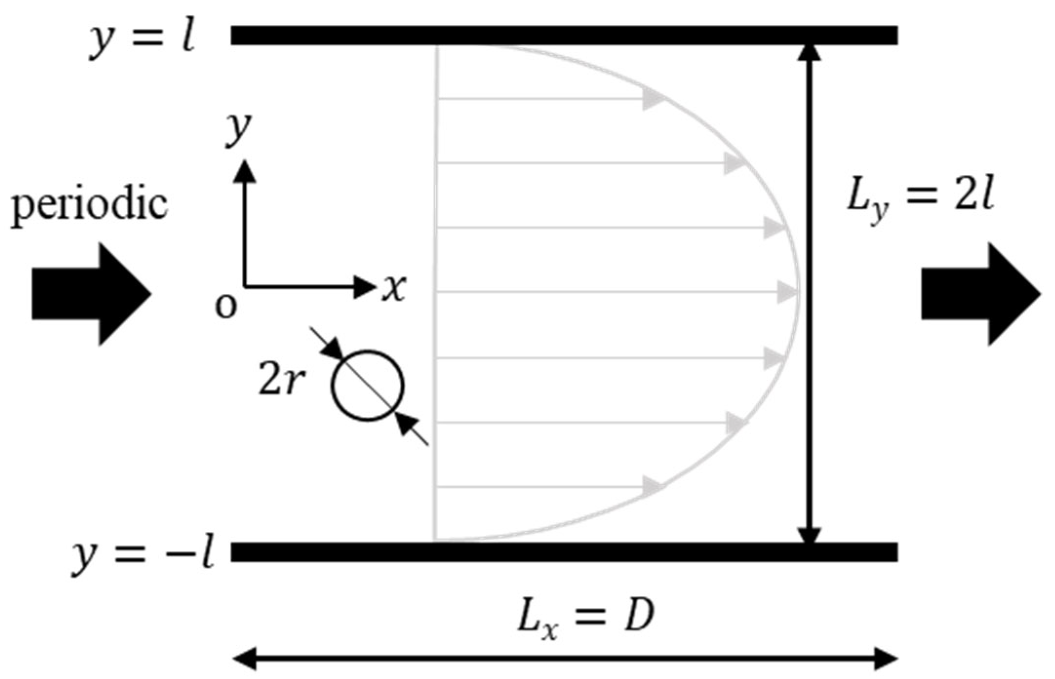
In this study, we analyzed two-dimensional flow using a two-way coupling scheme [17]. Figure 1 shows the numerical model of this study. Channel width is , and channel length is . We made channel width equal to channel length, and the grid resolution was set to . Then, the periodic boundary condition [17] was applied in the flow direction. We used Newtonian fluid, dilatant fluid, pseudoplastic fluid, and Bingham fluid. Regarding Reynolds number, Stickel and Powell indicated that inertial effects are important in the case of the particle Reynolds number [2]. The particle Reynolds number is defined as follows [18]:
where is the particle diameter and is the particle confinement. In this study, in order to consider particle inertial effects, Reynolds number was set to 32, i.e., the particle Reynolds number . These are the same conditions as that of the previous study [12]. We used a circular rigid particle with a diameter of as a suspended particle in this study. The confinement that represents particle size to the channel size , 0.10, 0.20, and 0.25. We used the virtual flux method [18,19,20,21] to express a rigid particle on a Cartesian grid. In this study, simulations were performed until non-dimensional time , and the simulations of lift force and relative viscosity were performed at every -axis position of the particle until non-dimensional time fixed the particle -axis position considering only the -axis translational motion and rotational motion. We did not treat a rigid suspended particle as colloids, and we do not consider the Brownian motion because the particle was sufficiently large and we considered that a particle only receives fluid force.

Figure 1.
Schematic view of a rigid suspended particle in a pressure-driven flow through a 2D channel. The initial position of a particle is changeable.
2.2. Governing Equation for Fluids
In this study, we used the regularized lattice Boltzmann equation [22,23] as a governing equation. One of the advantages of this method is reducing the amount of memory usage in the analysis. In this method, pressure distribution function is expressed using equilibrium pressure distribution function and non-equilibrium part of the pressure distribution function , as in Equation (3).
where is the discrete velocity vector, and is the relaxation time. The non-equilibrium part of the pressure distribution function and are obtained as follows:
where is the weight coefficient, is the speed of sound, is Kronecker’s delta, is the non-equilibrium part of the stress tensor, is the kinematic viscosity and apparent viscosity, is the shear rate, and is the lattice speed. In addition, the relationship between and is defined as . In this study, we chose relaxation time as .
2.3. Herschel–Bulkley Model
In this study, we used the Herschel–Bulkley model as a model that can express a non-Newtonian solvent [13,24]. This model can change solvent properties by changing the power-law index and Bingham number . In this model, the relationship between and is expressed as follows:
where is the yield stress, is the power-law consistency, is the characteristic length, and is the characteristic velocity. The power-law consistency in Equation (6) is derived from the following equation using Reynolds number :
Shear rate is derived from Equation (8) using second invariant of the strain stress tensor , and is derived from Equation (9) using the stress rate tensor :
Kinematic viscosity in Equation (5) is obtained from the following equation using Equation (8):
In Equation (10), when shear stress is less than yield stress, the shear rate is , and kinematic viscosity becomes discontinuous at the center of the channel. In order to eliminate this problem, Papanastasiou [25] proposed the following equation:
where is a constant to eliminate discontinuousness and is expressed as [26]. In this study, relaxation time in each lattice point is derived from Equation (5) using Equation (11).
2.4. Governing Equation for a Suspended Particle
In this study, we used a two-way coupling scheme [17] considering translational motion and rotational motion of suspended particle. Suspended particle motion is expressed by Newton’s second law for translational motion and angular equation for rotation as follows:
where are the external force vectors for particle, particle mass, position vector, torque, moment of inertia, and particle angle, respectively. Equations (12) and (13) are solved using the explicit third-order Adams–Bashforth method [27]. Then, we defined the force acting on a particle in the and directions as and , respectively, as follows:
where are the pressure, viscous stress, and small area, respectively, of the particle. Drag coefficient and lift coefficient are obtained using as follows:
where is the density, and is the particle radius. In this study, particle density is equal to fluid density because we studied a neutrally buoyant particle.
2.5. Relative Viscosity
The mass flow rate of a particle-free fluid in a Poiseuille flow with a well-developed boundary layer is obtained as follows:
where is the viscosity of particle-free fluid, and is the pressure difference over a channel length for particle-free fluid. The mass flow rate of a particle suspension is assumed to be obtained in the following equation in a similar way as Equation (18) [17]:
where is the effective viscosity, and is the pressure difference over a channel length for particle suspension. Therefore, when the relationship between mass flow rate of particle suspension and that of particle-free fluid is , the relative viscosity can be obtained from the following equation:
3. Results and Discussion
3.1. Validation for Velocity Profile and Apparent Viscosity without Particles
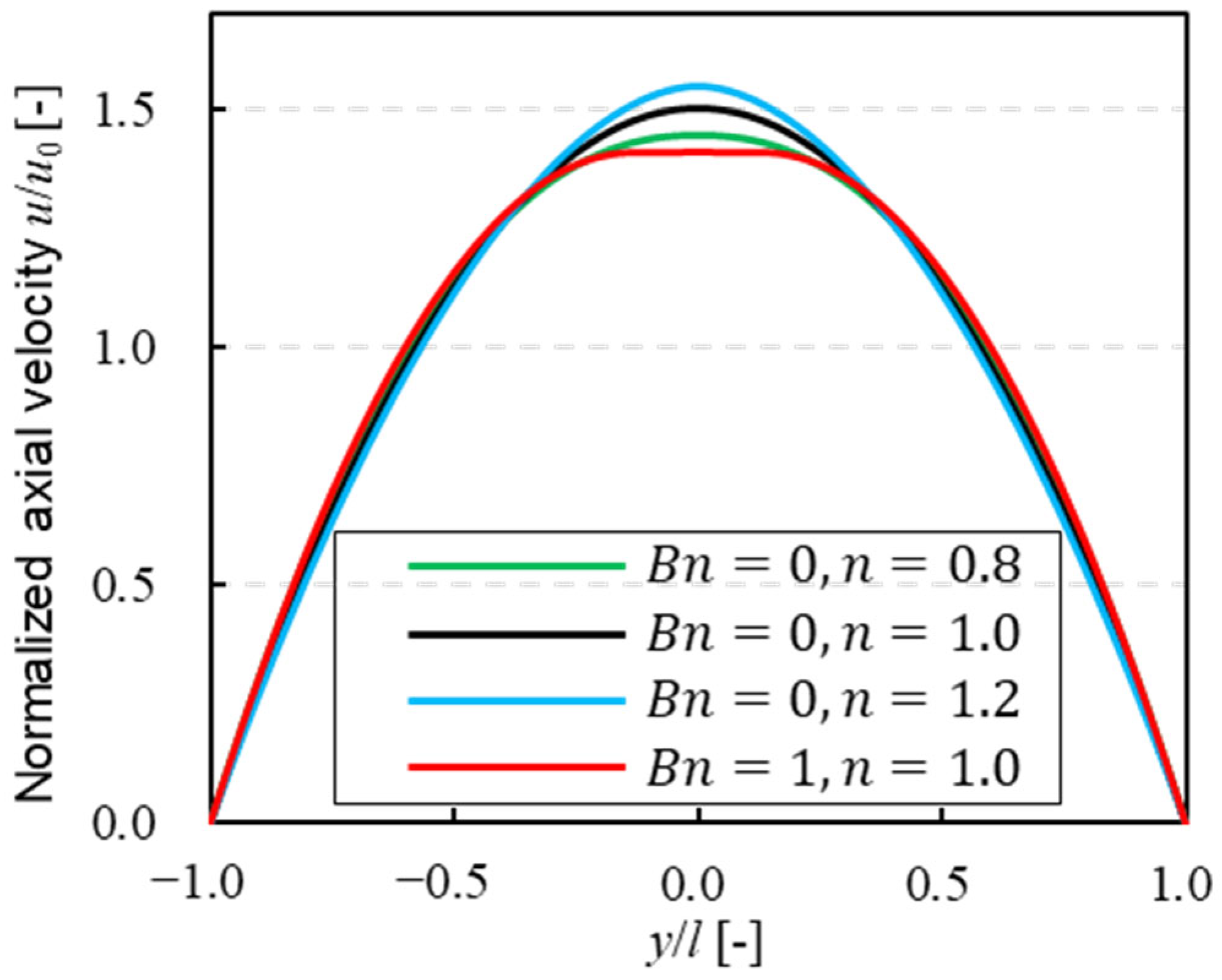
Figure 2 shows the results of the velocity profile of a particle-free fluid for each solvent. The green, black, and blue lines show power-law fluid , and the red line shows Bingham fluid , respectively. The velocity profile for power-law fluid in two-dimensional flow is expressed as follows [28]:
where is the velocity in the direction, and is half of the channel width. The error between the theoretical value and the analysis result was less than 1% for each solvent. In Bingham fluid, plug flow was confirmed near the center of the channel, as found in the previous study [26]. Figure 3 shows the apparent viscosity obtained from Equation (11). The result demonstrated that the apparent viscosity was higher near the channel center because the shear rate at the channel center in the direction was lower. Therefore, the red zone in Figure 3 shows the plug flow area, which was also observed by Mahmood et al. [29].

Figure 2.
Velocity profiles of power-law fluid and Bingham fluid in a channel without particles.
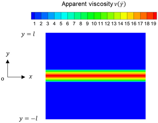
Figure 3.
Apparent viscosity distribution without particles in Bingham fluid .
3.2. Validation for Particle Migration in Power-Law Fluid
We confirmed the validity of the inertial migration of a particle using power-law fluid as a solvent. To compare the equilibrium position of a particle with that of previous studies, the channel length , which is different from that in Figure 1, was set to , Reynolds number was , confinement was , and power-law index took four values; . Reynolds number, confinement, and power-law index were the same as those used in previous studies [10] in order to compare with its results. Figure 4 shows the computed result of inertial migration of a particle, and the vertical and horizontal lines are the -axis position and non-dimensional time , respectively. This result suggested that the equilibrium position of a particle did not depend on the particle’s initial position. Then, we confirmed that the equilibrium position of the particle was closer to the center, as power-law index was higher. Table 1 shows a comparison between the numerical results and those from the previous study [10] and the difference between the two results. We obtained values close to those from previous studies and a similar tendency for each power-law index.
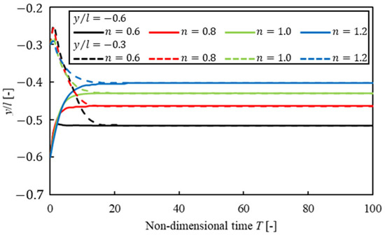
Figure 4.
Suspended particle migration trajectories for different power-law indices.

Table 1.
Equilibrium positions for different power-law indices.
3.3. Inertial Migration of a Suspended Particle Using Herschel–Bulkley Model
3.3.1. Dependence on Solvents
In this section, we investigated how a solvent affected the equilibrium position of a particle when confinement was the same. Figure 5 shows the migration history of a particle for each solvent when a particle started to flow at . The vertical line is the -axis position of a particle, and the horizontal line is non-dimensional time . Particle confinement is . The equilibrium position in Bingham fluid was closer to the wall than that in power-law fluid. The difference in the equilibrium position between pseudoplastic fluid and Bingham fluid was 0.06, which is less than half of a particle. We consider that these results were caused by the similarity of the velocity profile near the wall in pseudoplastic fluid and that in Bingham fluid in Figure 2.
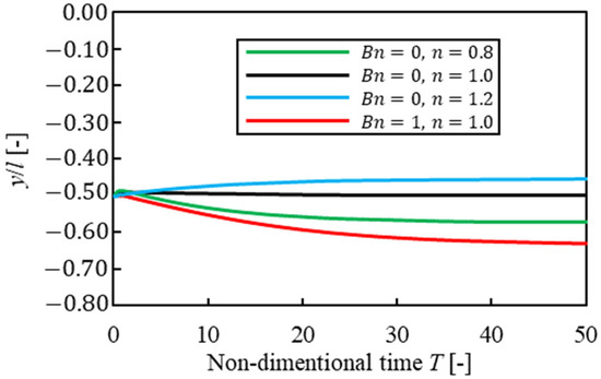
Figure 5.
Suspended particle migration trajectories for different solvents .
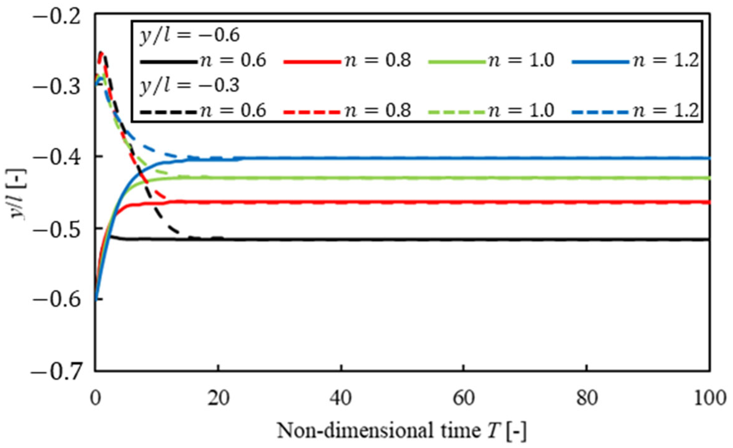
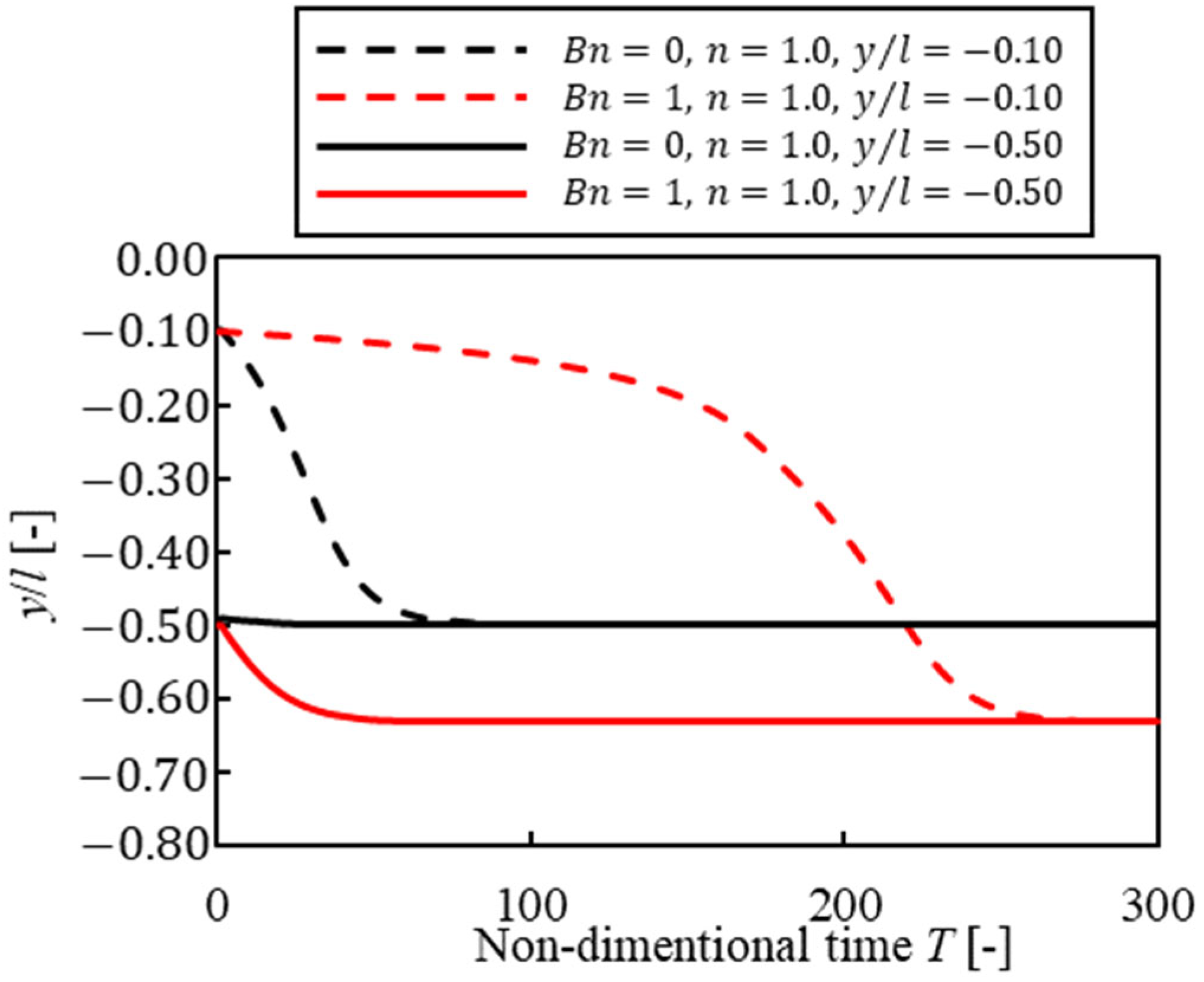
Next, Figure 6 shows the difference in migration history for each initial position. The vertical line is the -axis position of a particle, and the horizontal line is non-dimensional time . The dashed lines and the solid lines show the results of the particle’s initial positions of and , and the black lines and red lines show Newtonian fluid and Bingham fluid, respectively. In Bingham fluid, the equilibrium position did not depend on the initial position of a particle as in the case of Newtonian fluid. However, when a particle started to flow near the center of the channel, the time to reach the equilibrium position in Bingham fluid was three times as long as that in Newtonian fluid. We considered lift force acting on the particle, and the particle was difficult to move in the direction in plug flow that was seen in Figure 2. On the other hand, when a particle started to flow away from the center, the tendency of particle migration in Bingham fluid was similar to that in other solvents because shear rate was not 0 except at the center of the channel. Then, particle confinement was changed, and the particle began to flow near the center, as in . Figure 7 shows the result of , and Figure 8 shows that of . The vertical line is the -axis position of a particle, and the horizontal line is non-dimensional time . These results suggested that it was difficult for the particle to migrate near the center of the channel in Bingham fluid, similar to that of . However, the difference in the time for a particle to reach the equilibrium position was smaller than that of , because it was easier for a high-confinement particle to protrude from plug flow at the center, and it became more difficult for plug flow to affect particle migration. As a result, the equilibrium positions were Bingham, pseudoplastic, Newtonian, and dilatant fluids, in order, starting from the channel wall at each confinement. In other words, solvents had a greater influence on the equilibrium position than particle confinements. Thus, it was suggested that the choice of solvent affected particle migration.

Figure 6.
Suspended particle migration trajectories from different initial positions .
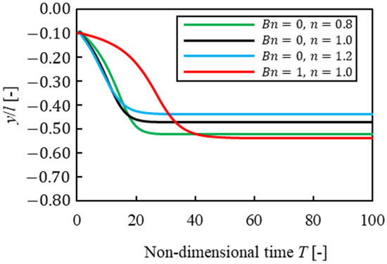
Figure 7.
Suspended particle migration trajectories for different solvents .
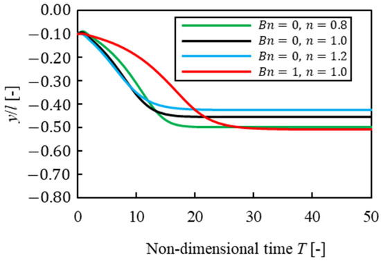
Figure 8.
Suspended particle migration trajectories for different solvents .
3.3.2. Dependence on Confinements
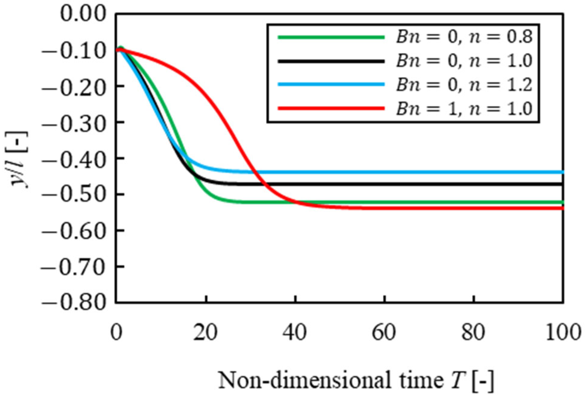
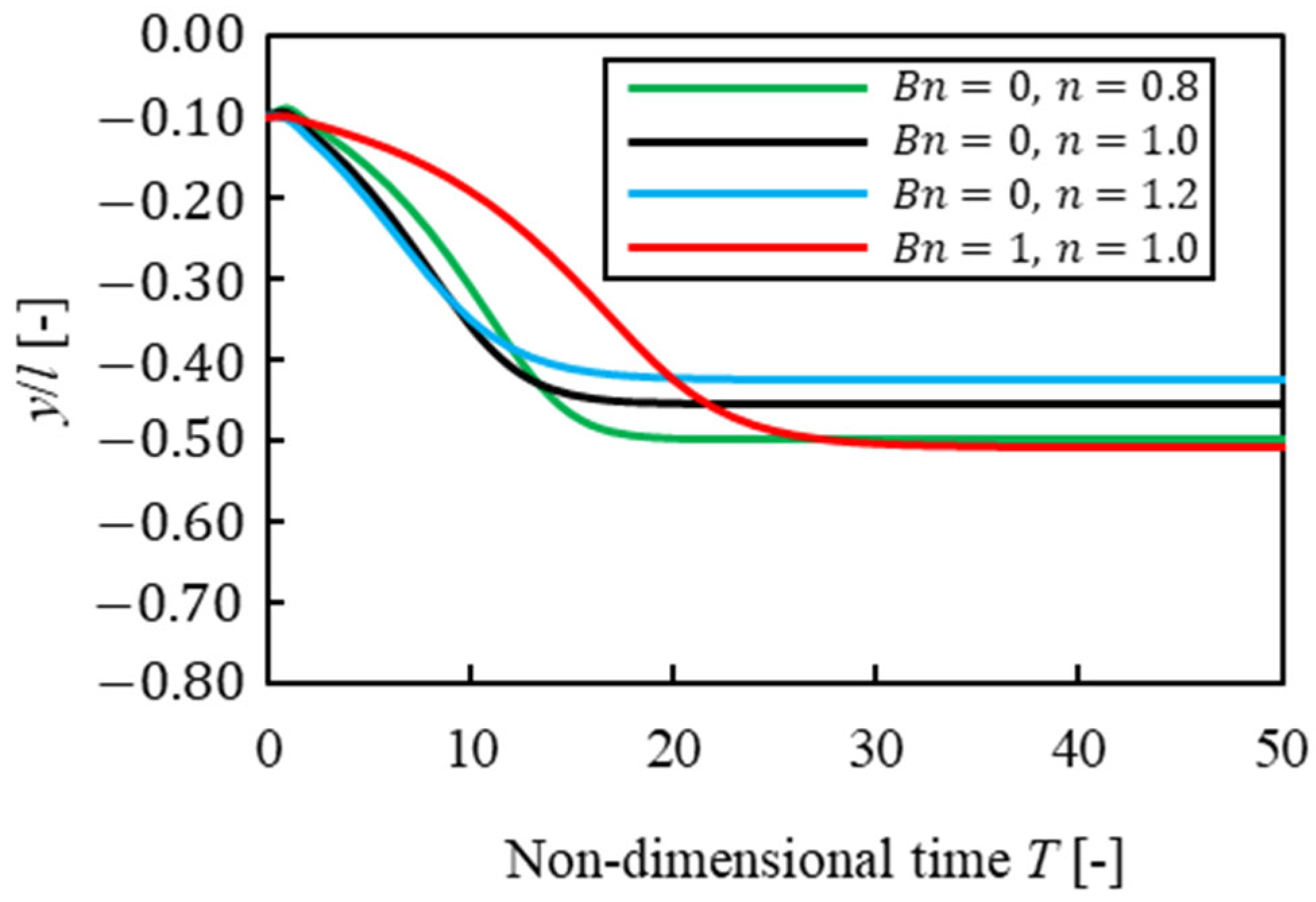
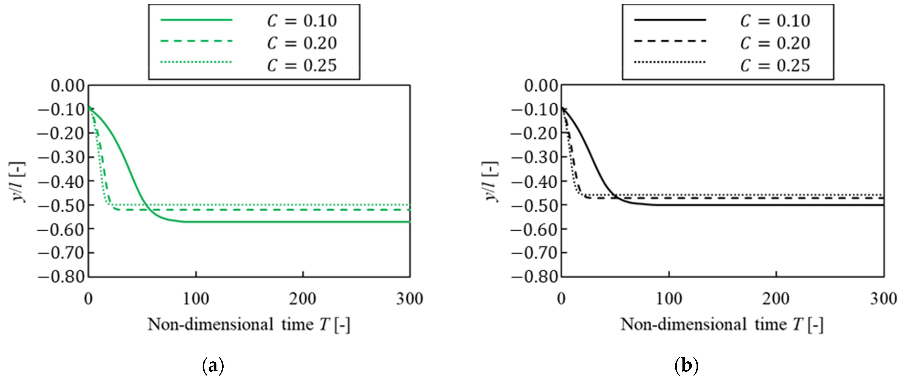
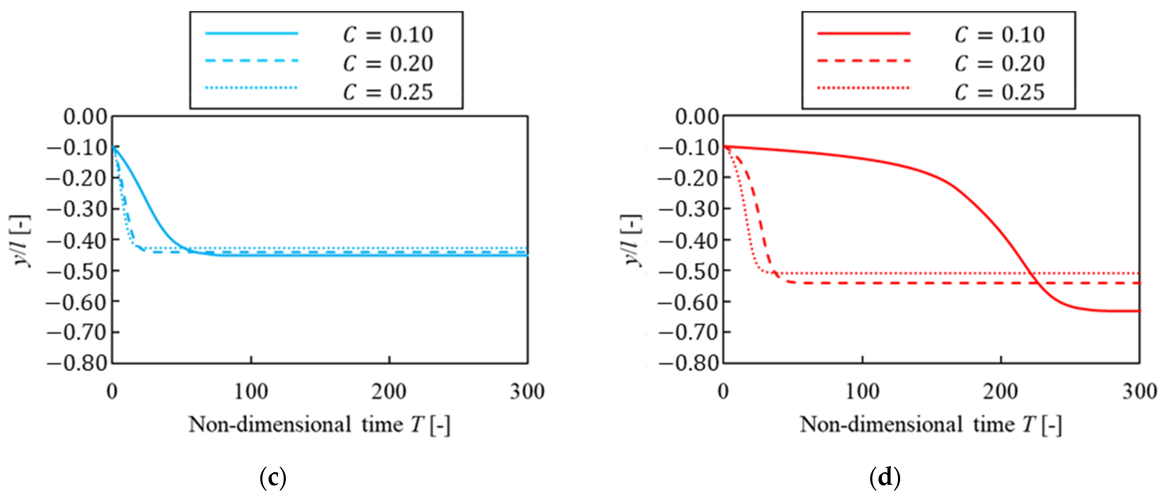
In this section, we investigate how confinement affected the equilibrium position when the solvent was the same. Figure 9 shows the migration history of a particle of three patterns of confinement () for each solvent; the vertical line is the -axis position, and the horizontal line shows non-dimensional time . For each solvent, how to migrate and the time until a particle reached the equilibrium position were not different in Figure 9a–d when confinement was . However, this time was longer in the case of than in . We consider that a particle had difficulty migrating to the equilibrium position because particle confinement was lower and lift force acting on a particle was lower, which means that fluid force acting on a particle was lower as particle confinement became lower. Moreover, as mentioned in Section 3.3.1, the time to reach the equilibrium position for was about three and a half times and seven times, respectively, as long as that for in Figure 9d. Therefore, it was suggested that a lower confinement particle was more affected by plug flow.
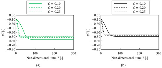
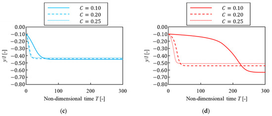
Figure 9.
Suspended particle migration trajectories for different confinements. (a) ; (b) ; (c) ; (d) .
3.4. Lift Force Acting on a Particle
3.4.1. Dependence on Solvents
In this section, we consider the relationship between lift force and the equilibrium position of a particle by investigating how a solvent affected lift force acting on a particle in an inertial flow. The simulation was performed fixing the particle’s -axis position and only translational motion and rotational motion were considered. Figure 10, Figure 11 and Figure 12 show the lift coefficient for each -axis position of a particle when confinement was ; the vertical line is lift coefficient , and the horizontal line shows the axis position. There were two points that had a lift coefficient : at the center of the channel and near the wall for each solvent and confinement. We found that the point that lift coefficient near the wall corresponded with the equilibrium position in Figure 9. The lift coefficient profile in power-law fluid was a convex upward parabola in any confinement. On the other hand, the lift coefficient profile in Bingham fluid was convex downward at and convex upward at . Moreover, the lift coefficient in Bingham fluid was lower at and higher at than that in power-law fluid. We found that in Bingham fluid, it was difficult for a particle was to migrate to the wall when a particle was near the center of the channel and vice versa. We considered that this effect may cause the difference in trajectories from different initial positions of a particle in Figure 6 when confinement . Therefore, it was suggested that plug flow in Bingham fluid also affected lift force acting on a particle and that this effect contributed to particle migration.

Figure 10.
Lift coefficient for different solvents . Note that the straight black line represents .

Figure 11.
Lift coefficient for different solvents . Note that the straight black line represents .
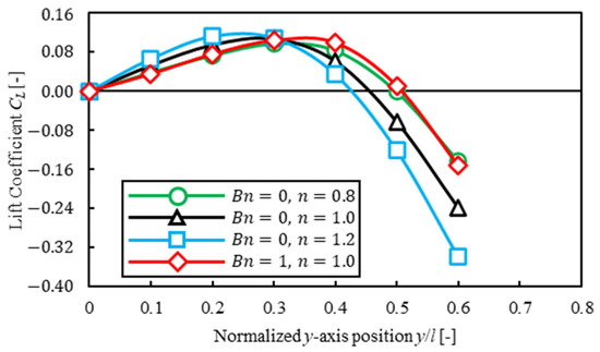
Figure 12.
Lift coefficient for different solvents . Note that the straight black line represents .
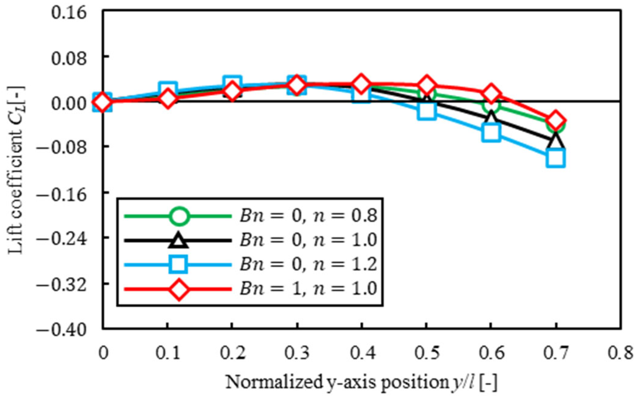
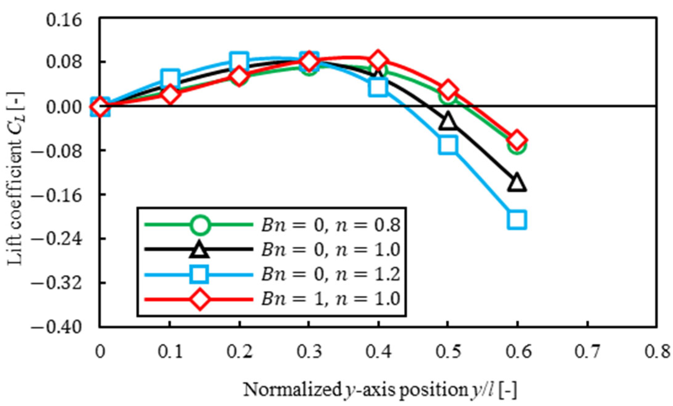
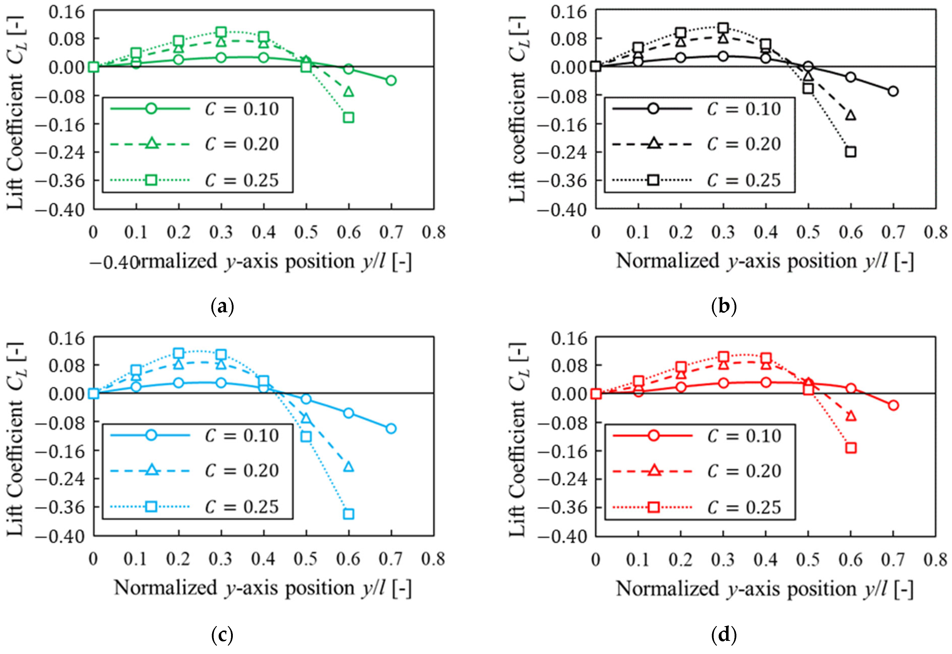
3.4.2. Dependence on Confinements
In this section, we investigated how confinement affected lift force acting on a particle when a solvent was the same. Figure 13 shows the lift coefficient of three patterns of confinement, , for each solvent. The vertical line is the lift coefficient , and the horizontal line shows the -axis position. We found that lift coefficient was higher for each solvent as confinement was higher. This result caused the force from the fluid to become stronger because the particle confinement was higher.

Figure 13.
Lift coefficient for different confinements. (a) ; (b) ; (c) ; (d) . Note that the straight black line represents .
As a result, the position where lift coefficient was closer to the center as confinement was higher. It was suggested that lift force acting on a particle was closely associated with the equilibrium position of a particle because the equilibrium position was closer to the wall as particle confinement was higher in Figure 9.
3.5. Relative Viscosity
3.5.1. Dependence on Solvents
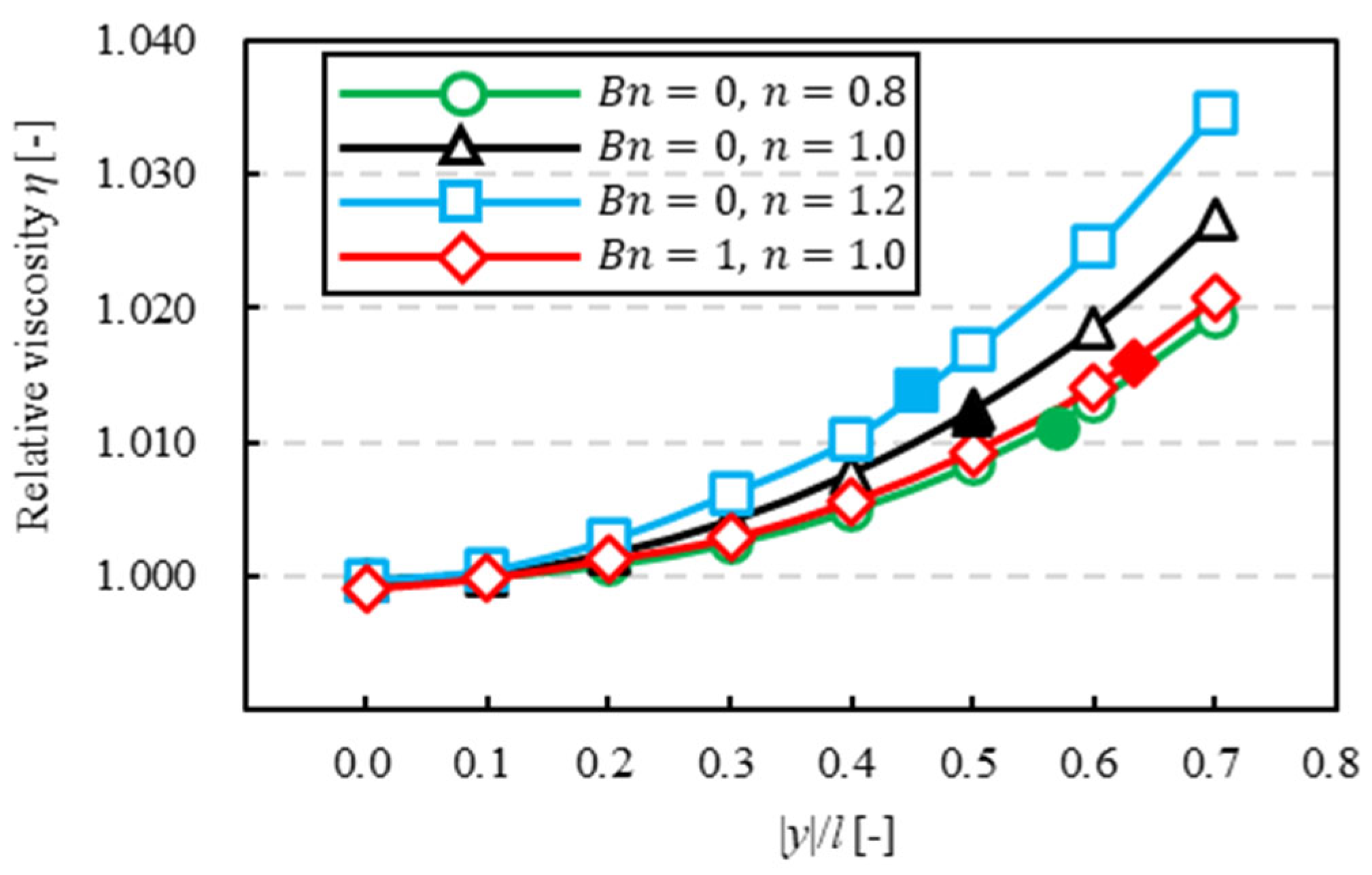
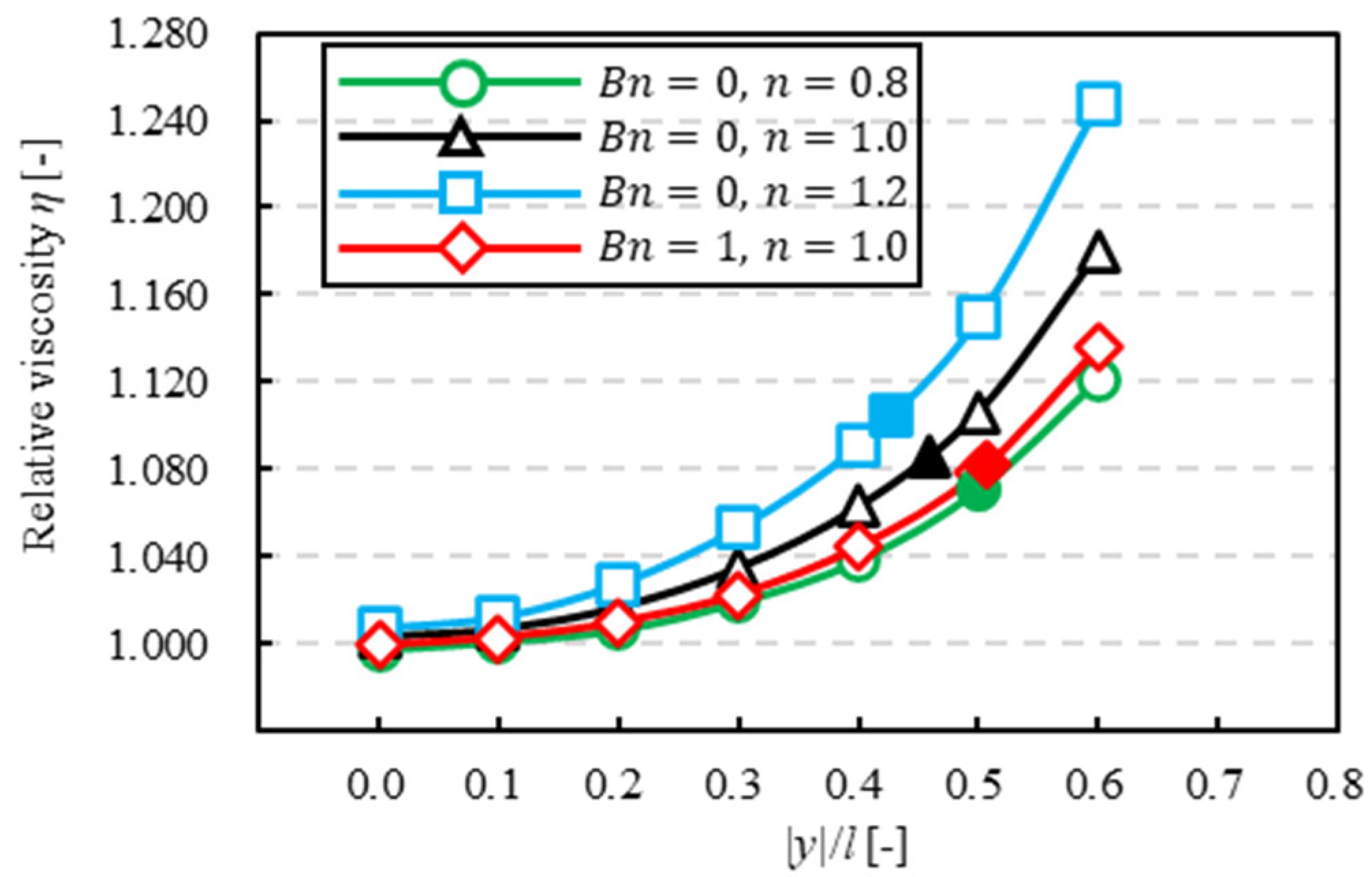
In this section, we investigate how a solvent affected relative viscosity. Figure 14, Figure 15 and Figure 16 show the relationship between the -axis position of a particle and relative viscosity for the same confinement. The vertical line is relative viscosity , and the horizontal line is the -axis position of a particle. In Figure 14, Figure 15 and Figure 16, the closed symbol is relative viscosity when a particle is at the equilibrium position and the open symbols are that when we fixed the -axis position of a particle as the same as that in the analysis of Section 3.4. Relative viscosity, when a particle is at the same -axis position and a solvent was different, was higher in the order of dilatant . Tanaka et al. [11] reported that when particles were regularly distributed using power-law fluid, relative viscosity was higher in the order of dilatant fluid Newtonian fluid Bingham fluid pseudoplastic fluid , and it was suggested that relative viscosity became higher as power-law index was higher when a particle at the same axis position and a solvent was different.
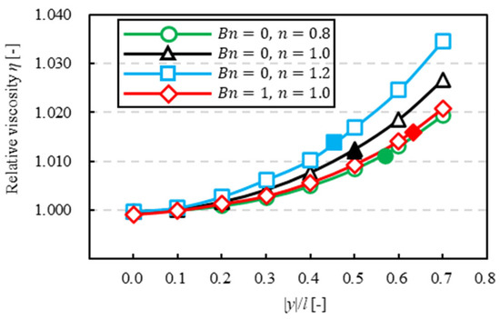
Figure 14.
Relative viscosity for different solvents . Note that the closed symbols are the particle at the equilibrium position.
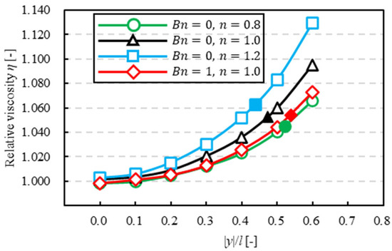
Figure 15.
Relative viscosity for different solvents . Note that the closed symbols are the particle at the equilibrium position.
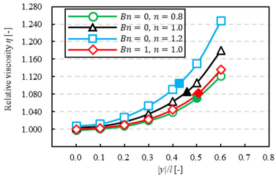
Figure 16.
Relative viscosity for different solvents . Note that the closed symbols are the particle at the equilibrium position.
Then, as a particle flowed farther away from the center of the channel, relative viscosity became higher for each solvent. This result is similar to the previous study using Newtonian fluid by Okamura et al. [7], and we consider that this tendency was seen when a solvent is a non-Newtonian fluid. The value of relative viscosity in Bingham fluid is close to that in pseudoplastic fluid. We consider that these results were caused by similarity of the velocity profile near the channel wall in pseudoplastic fluid and Bingham fluid , which suggests that shear velocity near the channel wall in the direction affected relative viscosity similarly to the particle equilibrium position. On the other hand, velocity profile near the channel center in Bingham fluid was completely different from that in pseudoplastic fluid , but the value of relative viscosity in Bingham fluid is close to that in pseudoplastic fluid near the channel center. We consider that the particle near the channel center did not contribute to the increase in relative viscosity. Thus, these results suggest that plug flow did not affect relative viscosity when the particle was near the channel center.
3.5.2. Dependence on Confinements
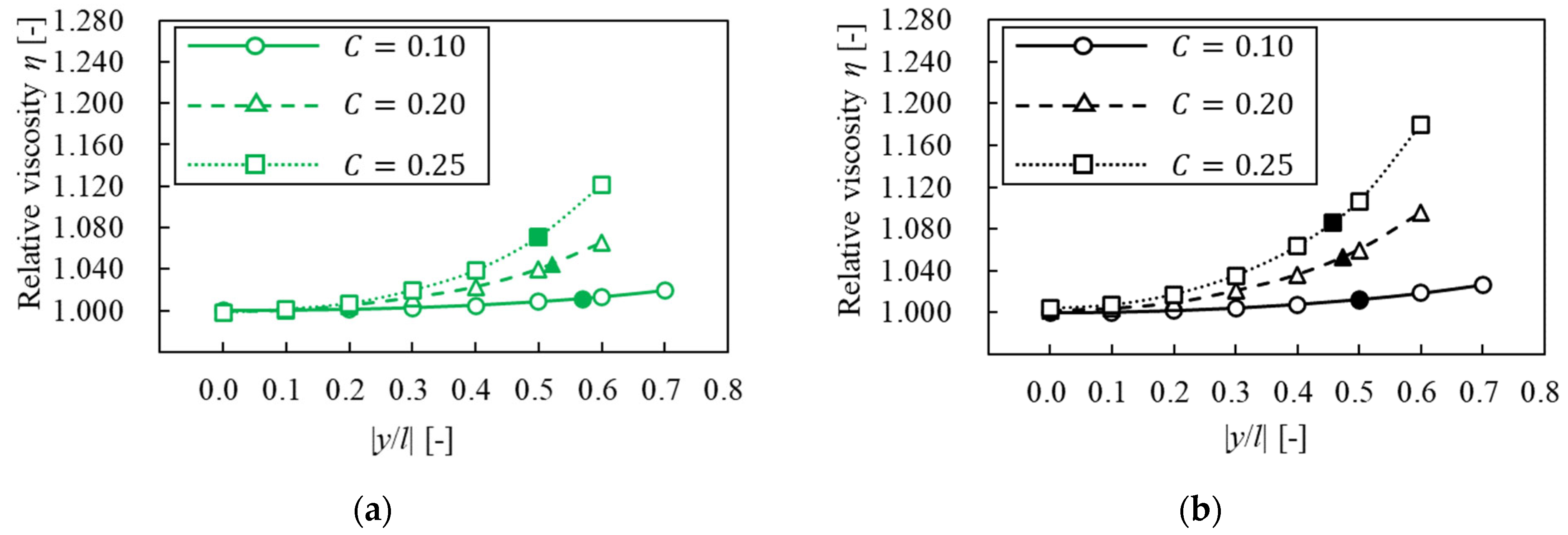
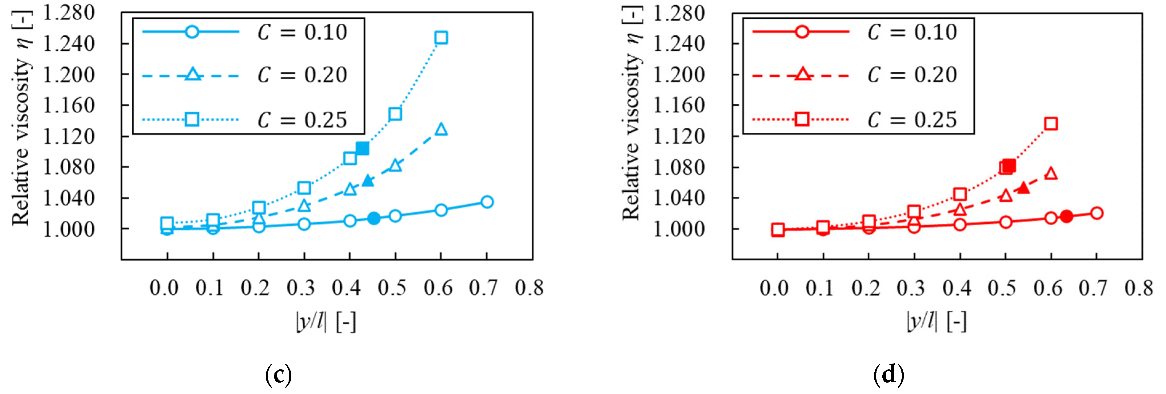
In this section, we investigated how confinement affected relative viscosity when a solvent was the same. Figure 17 shows the relationship between -axis position of a particle and relative viscosity. The vertical line is relative viscosity and the horizontal line is -axis position of a particle, where the closed symbol is relative viscosity when a particle is at the equilibrium position and the open symbols that when we fixed the -axis position of a particle in the same as the analysis in Section 3.4. When a particle was at the same -axis position, relative viscosity became higher for each solvent, as confinement was higher. This result was similar to that of Okamura et al. [7]. Therefore, it was suggested that relative viscosity in a non-Newtonian solvent was higher, as the area was greater with an increase in particle confinement.
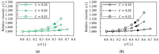
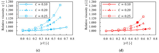
Figure 17.
Relative viscosity for different confinements. (a) ; (b) ; (c) ; (d) . Note that the closed symbols are the particle at the equilibrium position.
4. Conclusions
In this study, we investigated how non-Newtonian properties of a solvent affected the equilibrium position of a suspended particle and relative viscosity in two-dimensional parallel plate flow.
- We confirmed that the equilibrium position in Bingham fluid was closer to the wall than that in power-law fluid. Moreover, when a particle started to flow near the channel center, it was difficult for a particle in Bingham fluid to migrate in the direction and it spend more time reaching the equilibrium position than that in power-law fluid. These results were mainly caused by the velocity profile of a particle-free fluid, which indicates that shear rate near the wall and plug flow at the center of the channel strongly affected particle migration.
- When a particle was near the center, trajectories of migration in Bingham fluid were different from that in power-law fluid because of the different lift coefficient profile for each solvent.
- The tendency of relative viscosity, including that of a suspended particle in Bingham fluid was similar to that in pseudoplastic fluid. However, when the particle was at the equilibrium position, relative viscosity in Bingham fluid was different from that in pseudoplastic fluid.
Thus, it was suggested that the difference in solvents affected particle motion and relative viscosity for each particle position. In the future, based on these results for a single suspended particle, we will consider particle–particle interactions in suspension flow including multiple particles, and investigate complex effects on particle migration and relative viscosity.
Author Contributions
Conceptualization, K.T. and T.F.; methodology, K.T. and T.F.; software, K.T. and T.F.; validation, K.T.; formal analysis, K.T.; investigation, K.T.; resources, T.F.; data curation, K.T.; writing—original draft preparation, K.T.; writing—review and editing, K.T. and T.F.; visualization, K.T.; supervision, T.F.; project administration, T.F.; funding acquisition, T.F. All authors have read and agreed to the published version of the manuscript.
Funding
This work was supported by JSPS KAKENHI Grand Number JP20K04266 and Ihara Science Nakano Memorial Foundation.
Data Availability Statement
Data are contained within the article.
Conflicts of Interest
The authors declare no conflicts of interest.
References
- Gamonpilas, C.; Morris, J.F.; Denn, M.M. Shear and normal stress measurements in non-Brownian monodisperse and bidisperse suspensions. J. Rheol. 2016, 60, 289–296. [Google Scholar] [CrossRef]
- Stickel, J.J.; Powell, R.L. Fluid mechanics and rheology of dense suspensions. Annu. Rev. Fluid Mech. 2005, 37, 129–149. [Google Scholar] [CrossRef]
- Picano, F.; Breugem, W.-P.; Brandt, L. Turbulent channel flow of dense suspensions of neutrally-buoyant spheres. J. Fluid Mech. 2015, 764, 463–487. [Google Scholar] [CrossRef]
- Einstein, A. Eine neue Bestimmung der Moleküldimensionen. Ann. Der Physik 1906, 324, 289–306. [Google Scholar] [CrossRef]
- Brady, J.F. The Einstein viscosity correction in n dimensions. Int. J. Multiph. Flow 1983, 10, 113–114. [Google Scholar] [CrossRef]
- Segré, G.; Silberberg, A. Radial particle displacements in Poiseuille flow of suspensions. Nature 1961, 189, 209–210. [Google Scholar] [CrossRef]
- Okamura, N.; Fukui, T.; Kawaguchi, M.; Morinishi, K. Influence of each cylinder’s contribution on the total effective viscosity of a two-dimensional suspension by a two-way coupling scheme. J. Fluid Sci. Technol. 2021, 16, JFST0020. [Google Scholar] [CrossRef]
- Chen, D.; Lin, J. Steady State of Motion of Two Particles in Poiseuille Flow of Power-Law Fluid. Polymers 2022, 14, 2368. [Google Scholar] [CrossRef] [PubMed]
- Mueller, S.; Llewellin, E.W.; Mader, H.M. The rheology of suspensions of solid particles. Proc. Math. Phys. 2010, 466, 1201–1228. [Google Scholar] [CrossRef]
- Hu, X.; Lin, J.; Ku, X. Inertial migration of circular particles in Poiseuille flow of a power-law fluid. Phys. Fluids 2019, 31, 073306. [Google Scholar] [CrossRef]
- Tanaka, M.; Fukui, T.; Kawaguchi, M.; Morinishi, K. Numerical simulation on the effects of power-law fluidic properties on the suspension rheology. J. Fluid Sci. Technol. 2021, 16, JFST0022. [Google Scholar] [CrossRef]
- Masuyama, N.; Fukui, T. Numerical simulation of the effects of non-Newtonian property of the solvent on particle suspension rheology. Adv. Mech. Eng. 2023, 15, 16878132231198338. [Google Scholar] [CrossRef]
- Sobhani, S.M.J.; Bazargan, S.; Sadeghy, K. Sedimentation of an elliptic rigid particle in a yield-stress fluid: A Lattice-Boltzmann simulation. Phys. Fluids 2019, 31, 081902. [Google Scholar] [CrossRef]
- Chaparian, E.; Ardekani, M.N.; Brandt, L.; Tammisola, O. Particle migration in channel flow of an elastoviscoplastic fluid. J. Non-Newton. Fluid Mech. 2020, 284, 104376. [Google Scholar] [CrossRef]
- Siqueira, I.R.; De Souza Mendes, P.R. On the pressure-driven flow of suspensions: Particle migration in apparent yield-stress fluids. J. Non-Newton. Fluid Mech. 2019, 265, 92–98. [Google Scholar] [CrossRef]
- Herschel, W.H.; Bulkley, R. Konsistenzmessungen von Gummi-Benzollösungen. Kolloid-Z. 1926, 39, 291–300. [Google Scholar] [CrossRef]
- Fukui, T.; Kawaguchi, M.; Morinishi, K. A two-way coupling scheme to model the effects of particle rotation on the rheological properties of a semidilute suspension. Comput. Fluids 2018, 173, 6–16. [Google Scholar] [CrossRef]
- Miura, K.; Itano, T.; Sugihara-Seki, M. Inertial migration of neutrally buoyant spheres in a pressure-driven flow through square channels. J. Fluid Mech. 2014, 749, 320–330. [Google Scholar] [CrossRef]
- Tanno, I.; Morinishi, K.; Matsuno, K.; Nishida, H. Validation of virtual flux method for forced convection flow. JSME Int. J. Ser. B 2006, 49, 1141–1148. [Google Scholar] [CrossRef]
- Morinishi, K.; Fukui, T. An Eulerian approach for fluid -structure interaction problems. Comput. Fluids 2012, 65, 92–98. [Google Scholar] [CrossRef]
- Kawaguchi, M.; Fukui, T.; Morinishi, K. Comparative study of the virtual flux method and immersed boundary method coupled with regularized lattice Boltzmann method for suspension flow method. Comput. Fluids 2022, 246, 105615. [Google Scholar] [CrossRef]
- Izham, M.; Fukui, T.; Morinshi, K. Application of regularized lattice Boltzmann method incompressible flow simulation at high Reynolds number and flow with curved boundary. J. Fluid Sci. Technol. 2011, 6, 812–822. [Google Scholar] [CrossRef]
- Morinishi, K.; Fukui, T. Parallel computation of turbulent flows using moment base lattice Boltzmann method. Int. J. Comput. Fluid Dyn. 2016, 30, 363–369. [Google Scholar] [CrossRef]
- Gsell, S.; D’Ortona, U.; Favier, J. Lattice-Boltzmann simulation of creeping generalized Newtonian flows: Theory and guidelines. J. Comput. Phys. 2021, 173, 6–16. [Google Scholar] [CrossRef]
- Papanastasiou, T.C. Flows of viscoplastic materials: Models and Computations. Comput. Struct. 1997, 64, 677–694. [Google Scholar] [CrossRef]
- Chatzimina, M.; Georgiou, G.C.; Argyropaidas, I.; Mitsoulis, E.; Huilgo, R.R. Cessation of annular Poiseuille flows of Bingham plastics. J. Nonnewton. Fluid Mech. 2005, 129, 117–127. [Google Scholar] [CrossRef]
- Sewell, G. The Numerical Solution of Ordinary and Partial Differential Equations; Academic Press: Cambridge, MA, USA, 1988; pp. 43–50. [Google Scholar]
- Boyd, J.; Buick, J.; Green, S. A Second-Order Accurate Lattice Boltzmann Non-Newtonian Flow Model. J. Phys. A Math. Gen. 2006, 39, 14241–14247. [Google Scholar] [CrossRef]
- Mahmood, R.; Kousar, N.; Usman, K.; Mahmood, A. Finite element simulations for stationary Bingham fluid flow past a circular cylinder. J. Braz. Soc. Mech. Sci. 2018, 40, 459. [Google Scholar] [CrossRef]


Disclaimer/Publisher’s Note: The statements, opinions and data contained in all publications are solely those of the individual author(s) and contributor(s) and not of MDPI and/or the editor(s). MDPI and/or the editor(s) disclaim responsibility for any injury to people or property resulting from any ideas, methods, instructions or products referred to in the content. |
© 2024 by the authors. Licensee MDPI, Basel, Switzerland. This article is an open access article distributed under the terms and conditions of the Creative Commons Attribution (CC BY) license (https://creativecommons.org/licenses/by/4.0/).