


Optimising Physics-Informed Neural Network Solvers for Turbulence Modelling: A Study on Solver Constraints Against a Data-Driven Approach


Abstract
1. Introduction
Formulation of the Problem
2. Periodic Hill
3. Methods
3.1. Data-Driven Model
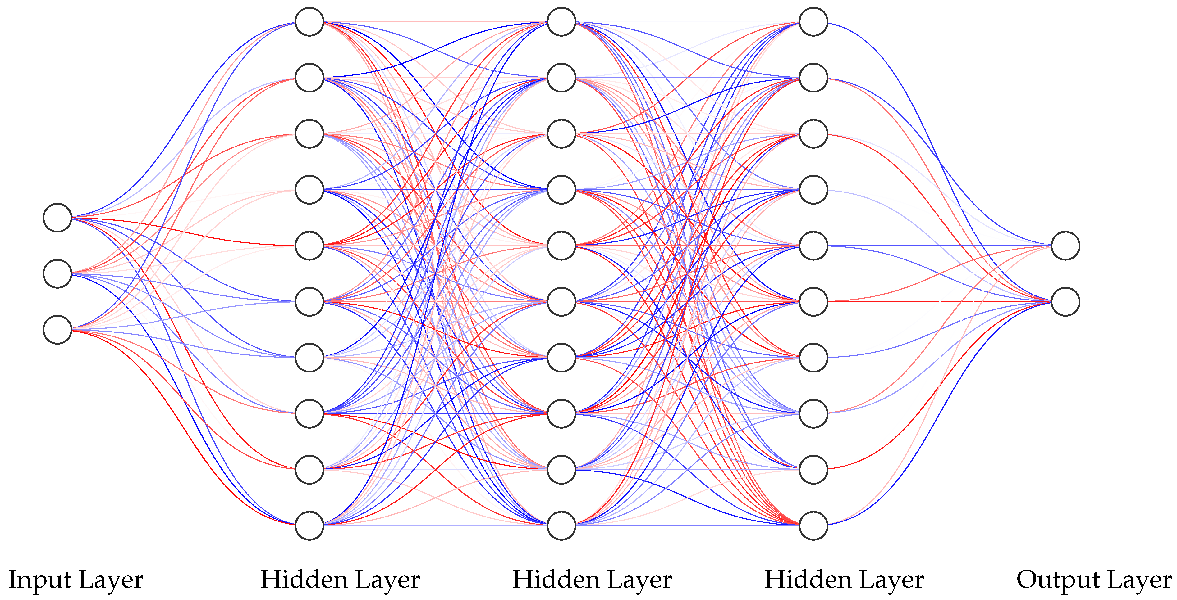
3.1.1. Network Architecture
3.1.2. Loss Function
3.1.3. Training
3.2. Physics-Informed Neural Network
3.2.1. Network Architecture
3.2.2. Loss Function
3.2.3. Training
3.2.4. Direct Reynolds Stress Model
3.2.5. Direct Reynolds Stress Model with Reduced Boundary Enforcement
3.2.6. Continuity Only Model
3.2.7. Mixing Length Model
3.2.8. Turbulent Viscosity Model
3.2.9. Turbulent Viscosity and Turbulent Kinetic Energy Model
3.2.10. Computation
3.3. Summary of PINNs Methods
4. Results
4.1. Data-Driven Model
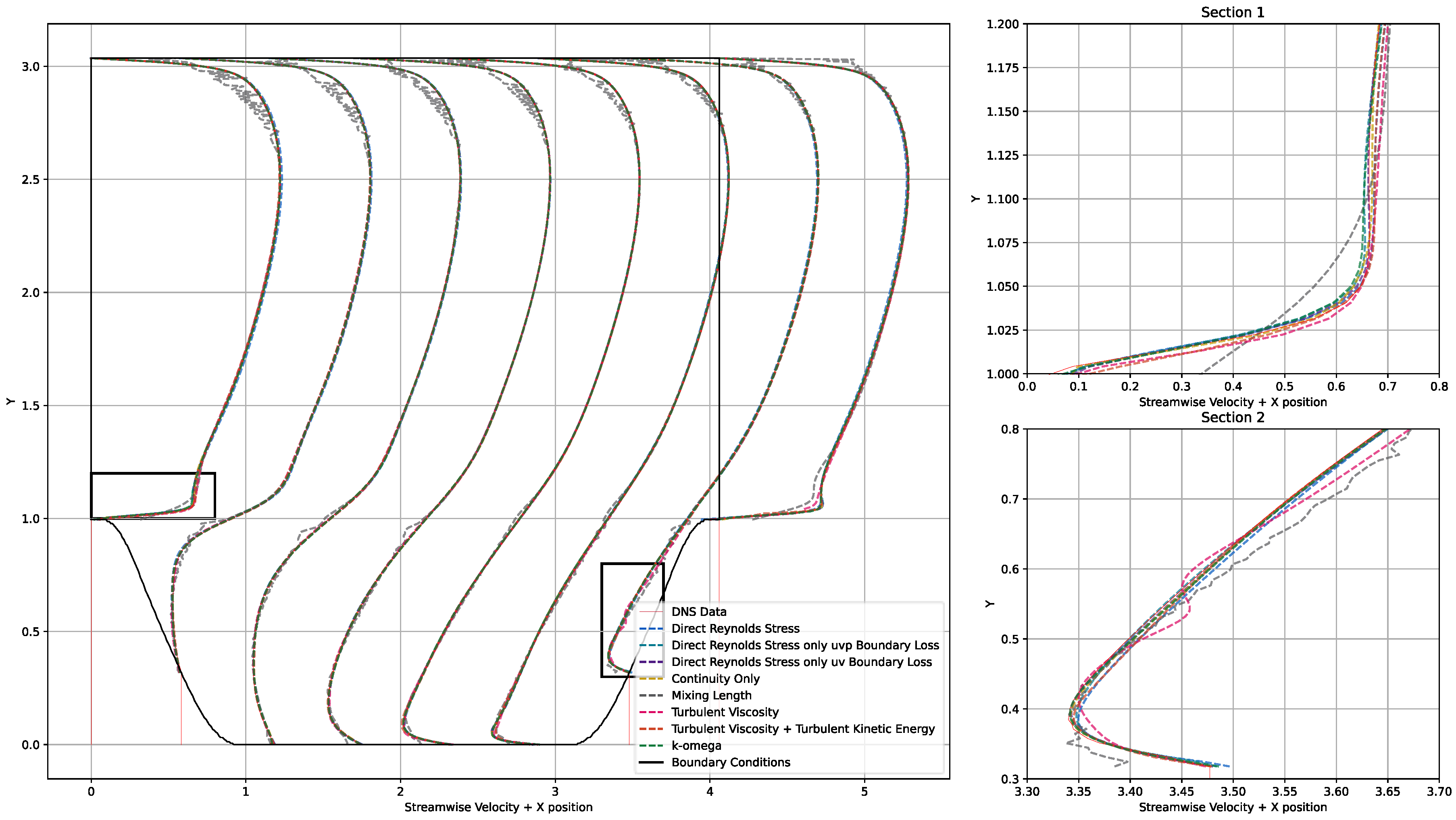
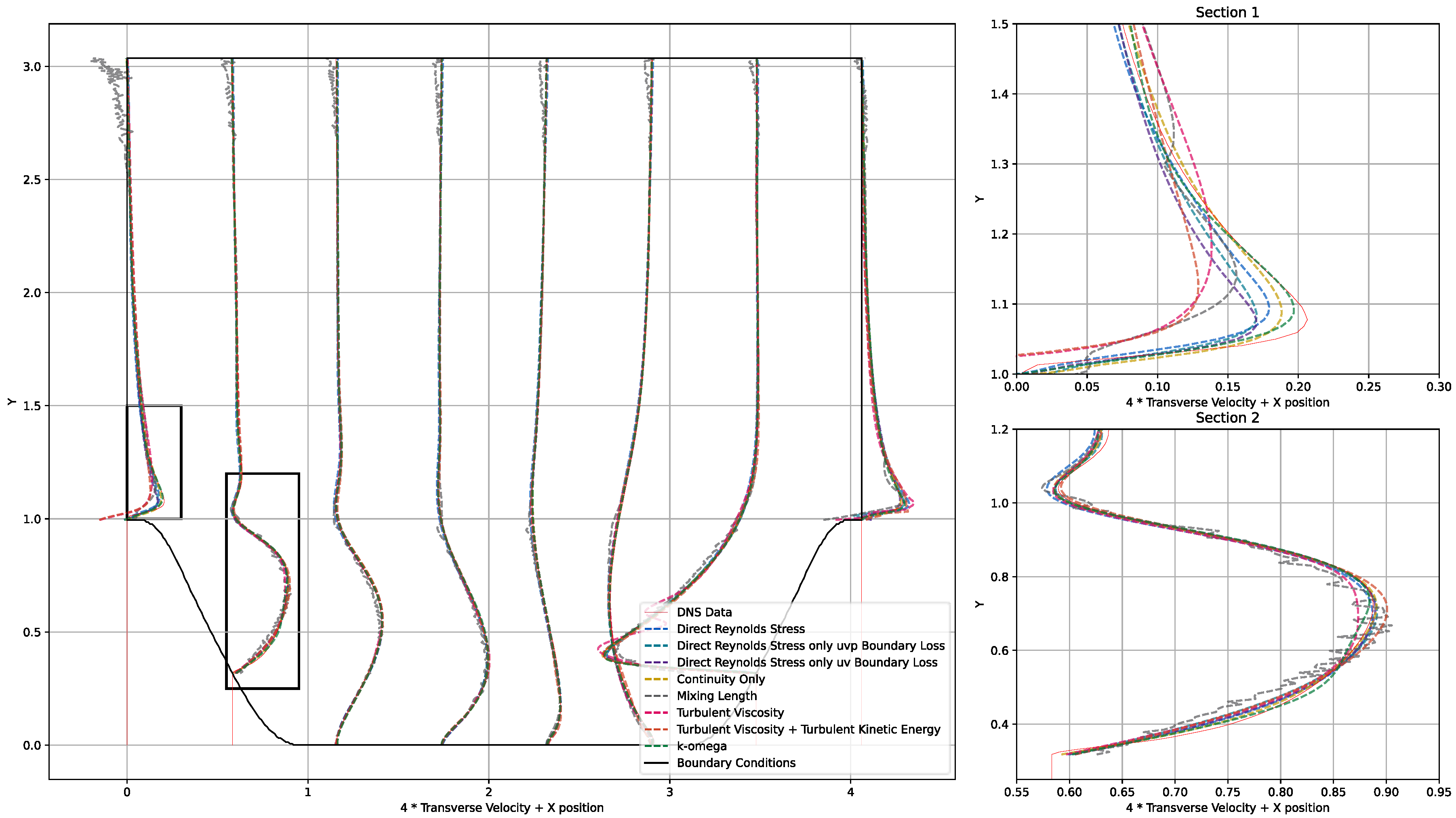
4.2. PINNs Models
5. Discussion
5.1. Data-Driven Model
5.2. PINNs Models
6. Conclusions
Author Contributions
Funding
Data Availability Statement
Conflicts of Interest
Abbreviations
| PINNs | Physics-informed neural network |
| CFD | Computational fluid dynamics |
| DNS | Direct numerical simulation |
| ROM | Reduced-order modelling |
| RANS | Reynold’s averaged Navier–Stokes |
| MLP | Multilayer perceptron |
| MAE | Mean averaged error |
| MSE | Mean squared error |
| DRSM | Direct Reynold’s stress model |
| RBMuvp | Direct Reynold’s stress model with reduced boundary enforcement of only u, v, and p |
| RBMuv | Direct Reynold’s stress model with reduced boundary enforcement of only u and v |
| COM | Continuity only model |
| MLM | Mixing length model |
| TVM | Turbulent viscosity model |
| TVKEM | Turbulent viscosity and turbulent kinetic energy model |
| KOM | K-Omega model |
| Bar indicates time-averaged component | |
| Prime indicates fluctuating component | |
| Time-averaged streamwise velocity | |
| Time-averaged transverse velocity | |
| Density (kg/m3) | |
| Kinematic viscosity (m2/s) | |
| First-order Reynold’s stress wrt. i and j | |
| Geometric slope parameter | |
| h | Domain height (m) |
| l | Domain length (m) |
| Dataset value | |
| Neural network predicted value | |
| Boundary-enforced variables | |
| Non-boundary-enforced variables | |
| Time-averaged pressure | |
| Turbulent viscosity (kg/ms) | |
| Stress tensor | |
| Kronecker delta | |
| k | Turbulent kinetic energy |
| d | Distance from the wall (m) |
| G | Strain tensor |
| Mixing length |
Appendix A
Appendix A.1. 2D Stationary Equations—Continuity
Appendix A.2. 2D Stationary Equations—Momentum in x and y
Appendix A.3. Mixing Length Model
Appendix A.4. K-Omega Model
Appendix B
- where and are normalised horizontal and vertical coordinates, respectively.
Appendix C
Appendix D
Appendix D.1. Methods
Appendix D.2. KOM Model

| Method Name | Neural Network Inputs | Neural Network Outputs | Governing Flow Equations | Enforced Boundaries |
|---|---|---|---|---|
| K-Omega | 2D turbulent kinetic energy stationary: 2D turbulent kinetic energy dissipation stationary: Turbulent viscosity: Turbulent kinetic energy dissipation rate limit: First-order stresses: |
| Neural Network Name | Neural Network Abbreviation | Training Time (s) | Prediction Time | Error (%) * | Error (%) * | Error (%) * | Description |
|---|---|---|---|---|---|---|---|
| K-Omega Model | KOM | 1.83 | - | 0.161 | 2.28 | - | Learning Rate of 1 × 10⁻² required for convergence, compared with 1 × 10⁻³ for rest. Compared with others, time should be slower than shown. |
Appendix D.3. KOM Results
Appendix D.4. KOM Discussion
Appendix E
Appendix F
| Testing Geometry (Filename) | Run 1 Time (hrs) | Run 2 Time (hrs) | Run 3 Time (hrs) | Run 1 Epochs | Run 2 Epochs | Run 3 Epochs |
|---|---|---|---|---|---|---|
| 05-10071-2024 | 4.1465 | 4.8044 | 2.3025 | 64 | 75 | 36 |
| 05-10071-3036 | 4.2917 | 6.0054 | 3.6440 | 71 | 100 | 60 |
| 05-10071-4048 | 6.4153 | 4.5389 | 3.6440 | 100 | 72 | 58 |
| 05-4071-2024 | 6.5736 | 6.5935 | 6.5516 | 100 | 100 | 100 |
| 05-4071-3036 | 3.1383 | 3.3755 | 2.1277 | 51 | 54 | 34 |
| 05-4071-4048 | 6.4042 | 3.8653 | 4.8055 | 98 | 58 | 75 |
| 05-7071-2024 | 6.1510 | 6.2457 | 6.1696 | 100 | 100 | 100 |
| 05-7071-3036 | 6.0619 | 2.7623 | 5.9172 | 100 | 44 | 95 |
| 05-7071-4048 | 6.0049 | 6.1623 | 4.4935 | 98 | 100 | 73 |
| 075-80355-3036 | 2.1614 | 2.0215 | 3.5191 | 35 | 32 | 57 |
| 10-12-2024 | 4.0714 | 2.6690 | 6.3826 | 62 | 41 | 100 |
| 10-12-3036 | 3.3554 | 6.1844 | 3.9754 | 55 | 100 | 66 |
| 10-12-4048 | 3.9153 | 3.6145 | 2.6540 | 62 | 57 | 43 |
| 10-6-2024 | 1.9820 | 6.6085 | 6.2423 | 31 | 100 | 94 |
| 10-6-3036 | 4.1323 | 4.1945 | 6.1153 | 67 | 68 | 100 |
| 10-6-4048 | 2.5583 | 4.5273 | 4.4232 | 40 | 70 | 69 |
| 10-9-2024 | 2.9653 | 6.6347 | 2.7177 | 46 | 100 | 41 |
| 10-9-3036 | 2.1101 | 2.4105 | 2.9650 | 35 | 39 | 48 |
| 10-9-4048 | 3.6485 | 2.6676 | 6.5280 | 59 | 42 | 98 |
| 125-99645-3036 | 6.1283 | 6.2453 | 6.0690 | 100 | 100 | 100 |
| 15-10929-2024 | 4.5933 | 4.5386 | 4.1385 | 74 | 72 | 67 |
| 15-10929-3036 | 1.8833 | 6.0567 | 1.9385 | 31 | 100 | 32 |
| 15-10929-4048 | 2.3954 | 2.1975 | 2.0831 | 40 | 36 | 35 |
| 15-13929-2024 | 3.7073 | 2.3868 | 2.1093 | 59 | 37 | 33 |
| 15-13929-3036 | 2.9063 | 2.2772 | 2.6044 | 48 | 38 | 44 |
| 15-13929-4048 | 1.9373 | 2.0007 | 1.9445 | 31 | 32 | 31 |
| 15-7929-2024 | 2.2224 | 3.0369 | 3.5955 | 34 | 46 | 55 |
| 15-7929-3036 | 2.3923 | 1.9600 | 3.7755 | 39 | 32 | 61 |
| 15-7929-4048 | 3.9381 | 6.1410 | 3.5175 | 61 | 96 | 55 |
| Median Average | 3.6485 | 2.2772 | 3.7755 | 59 | 69 | 61 |
| Testing Geometry | Error (%) | Error (%) | Error (%) | ||||||
|---|---|---|---|---|---|---|---|---|---|
| (Filename) | Run 1 | Run 2 | Run 3 | Run 1 | Run 2 | Run 3 | Run 1 | Run 2 | Run 3 |
| 05-10071-2024 | 10.7 | 8.1 | 7.4 | 53.6 | 39.9 | 36.0 | 107.4 | 108.3 | 107.2 |
| 05-10071-3036 | 3.8 | 2.4 | 3.6 | 25.3 | 16.9 | 19.6 | 109.1 | 111.3 | 110.9 |
| 05-10071-4048 | 2.4 | 2.4 | 3.9 | 23.7 | 15.8 | 30.9 | 117.2 | 115.9 | 114.7 |
| 05-4071-2024 | 9.1 | 10.0 | 10.1 | 69.3 | 61.1 | 68.4 | 157.6 | 166.3 | 146.5 |
| 05-4071-3036 | 2.8 | 4.1 | 3.5 | 67.5 | 66.6 | 64.0 | 213.9 | 222.6 | 215.8 |
| 05-4071-4048 | 2.9 | 3.5 | 6.1 | 60.7 | 64.7 | 84.8 | 253.9 | 241.9 | 251.6 |
| 05-7071-2024 | 5.3 | 5.9 | 6.0 | 39.6 | 36.7 | 44.6 | 110.4 | 110.1 | 111.9 |
| 05-7071-3036 | 2.9 | 3.4 | 2.5 | 30.0 | 33.3 | 23.6 | 123.3 | 125.1 | 122.3 |
| 05-7071-4048 | 2.2 | 1.8 | 1.9 | 23.8 | 24.9 | 23.8 | 135.1 | 133.4 | 130.5 |
| 075-80355-3036 | 19.2 | 15.1 | 13.1 | 127.6 | 109.5 | 94.0 | 130.5 | 127.6 | 112.5 |
| 10-12-2024 | 8226.0 | 33.7 | 34.2 | 5213.0 | 113.8 | 116.5 | 7328.0 | 111.4 | 111.8 |
| 10-12-3036 | 19.3 | 15.6 | 14.9 | 77.7 | 86.9 | 61.3 | 113.0 | 110.9 | 111.8 |
| 10-12-4048 | 18.4 | 15.0 | 18.1 | 103.6 | 84.4 | 92.2 | 114.7 | 113.2 | 113.7 |
| 10-6-2024 | 17.4 | 16.9 | 15.6 | 117.0 | 114.0 | 112.5 | 118.2 | 117.7 | 118.0 |
| 10-6-3036 | 9.8 | 6.2 | 9.7 | 95.4 | 60.9 | 101.4 | 147.0 | 146.9 | 147.4 |
| 10-6-4048 | 10.0 | 9.4 | 9.3 | 146.4 | 133.7 | 135.0 | 174.7 | 175.0 | 178.9 |
| 10-9-2024 | 21.0 | 21.4 | 21.0 | 81.3 | 79.8 | 94.3 | 106.6 | 108.5 | 108.6 |
| 10-9-3036 | 14.8 | 14.0 | 10.0 | 90.0 | 88.4 | 49.9 | 114.9 | 114.0 | 114.6 |
| 10-9-4048 | 10.6 | 9.9 | 6.3 | 83.4 | 81.3 | 56.7 | 119.9 | 120.9 | 119.1 |
| 125-99645-3036 | 1169.5 | 34.7 | 28.6 | 1431.7 | 110.7 | 126.6 | 1372.3 | 96.5 | 102.4 |
| 15-10929-2024 | 12.0 | 10.1 | 10.4 | 39.2 | 33.9 | 39.0 | 103.6 | 103.6 | 103.3 |
| 15-10929-3036 | 18.4 | 5.0 | 4.6 | 87.3 | 29.1 | 26.0 | 106.3 | 106.9 | 106.3 |
| 15-10929-4048 | 5.5 | 5.4 | 5.3 | 30.2 | 26.4 | 31.6 | 106.6 | 107.5 | 108.5 |
| 15-13929-2024 | 31.4 | 7519.2 | 146,994.1 | 109.9 | 86,986.4 | 135,865.8 | 108.9 | 28,905.0 | 417,257.2 |
| 15-13929-3036 | 25.2 | 27.9 | 20.0 | 95.5 | 105.6 | 110.7 | 108.4 | 109.9 | 106.4 |
| 15-13929-4048 | 30.7 | 20.8 | 120.3 | 103.2 | 105.5 | 6150.2 | 110.5 | 110.7 | 184.9 |
| 15-7929-2024 | 25.4 | 25.5 | 23.6 | 98.6 | 98.6 | 91.0 | 104.4 | 104.7 | 105.4 |
| 15-7929-3036 | 17.7 | 18.9 | 18.0 | 97.9 | 97.8 | 99.0 | 111.8 | 110.1 | 111.6 |
| 15-7929-4048 | 14.0 | 14.3 | 14.9 | 110.3 | 94.2 | 98.7 | 119.5 | 118.3 | 116.7 |
| Median Average | 12.0 | 10.0 | 10.0 | 83.4 | 80.5 | 68.4 | 114.7 | 112.3 | 112.5 |
Appendix G

Appendix H
References
- Balakumar, P. Direct Numerical Simulation of Flows over an NACA-0012 Airfoil at Low and Moderate Reynolds Numbers. In Proceedings of the 47th AIAA Fluid Dynamics Conference, Hampton, VA, USA, 5–9 June 2017. [Google Scholar]
- Cenedese, M.; Axas, J.; Bauerlein, B.; Avila, K.; Haller, G. Data-driven modeling and prediction of non-linearizable dynamics via spectral submanifolds. Nat. Commun. 2022, 13, 872. [Google Scholar] [CrossRef] [PubMed]
- Lagaris, I.; Likas, A.; Fotiadis, D. Artificial neural networks for solving ordinary and partial differential equations. IEEE Trans. Neural Netw. 1998, 9, 987–1000. [Google Scholar] [CrossRef]
- Maissi, M.; Perdikaris, P.; Karniadakis, G. Physics Informed Deep Learning (Part I): Data-driven Solutions of Nonlinear Partial Differential Equations. arXiv 2017, arXiv:1711.10561. [Google Scholar]
- Jin, X.; Cai, S.; Li, H.; Karniadakis, G. NSFnets (Navier-Stokes flow nets): Physics-informed neural networks for the incompressible Navier-Stokes equations. J. Comput. Phys. 2021, 426, 109951. [Google Scholar] [CrossRef]
- Eivazi, H.; Tahani, M.; Schlatter, P.; Vinuesa, R. Physics-informed neural networks for solving Reynolds-averaged Navier-Stokes equations. Phys. Fluids 2022, 34, 07511. [Google Scholar] [CrossRef]
- Pioch, F.; Harmening, J.; Muller, A.; Peitzmann, F.; Schramm, D.; el Moctar, O. Turbulence Modeling for Physics-Informed Neural Networks: Comparison of Different RANS Models for the Backward-Facing Step Flow. Fluids 2023, 8, 43. [Google Scholar] [CrossRef]
- Lucas, H.; Bollhöfer, M.; Römer, U. Statistical reduced order modelling for the parametric Helmholtz equation. arXiv 2024, arXiv:2407.04438. [Google Scholar] [CrossRef]
- Fu, J.; Xiao, D.; Fu, R.; Li, C.; Zhu, C.; Arcucci, R.; Navon, I.M. Physics-Data Combined Machine Learning for Parametric Reduced-Order Modelling of Nonlinear Dynamical Systems in Small-Data Regimes; Zienkiewicz Centre for Computational Engineering, Swansea University: Swansea, UK, 2022. [Google Scholar]
- Brunton, S.L.; Proctor, J.L.; Kutz, J.N. Discovering Governing Equations from Data: Sparse Identification of Nonlinear Dynamical Systems. arXiv 2015, arXiv:1509.03580. [Google Scholar] [CrossRef] [PubMed]
- Martina, B.; Manojlović, I.; Muha, B.; Vlah, D. Deep Learning Reduced Order Modelling on Parametric and Data-driven Domains. arXiv 2024, arXiv:2407.17171. [Google Scholar] [CrossRef]
- Vinuesa, R.; Brunton, S.L. Enhancing Computational Fluid Dynamics with Machine Learning. FLOW, Engineering Mechanics; KTH Royal Institute of Technology: Stockholm, Sweden; Swedish e-Science Research Centre (SeRC): Stockholm, Sweden; Department of Mechanical Engineering, University of Washington: Seattle, WA, USA, 2022. [Google Scholar]
- Rudy, D.H.; Bushnell, D.M. A Rational Approach to the use of Prandtl’s Mixing Length Model in Free Turbulent Shear Flow Calculations. Nasa Langley Res. Cent. 1973, 1. [Google Scholar]
- Chipongo, K.; Khiadani, M.; Sookhak Lari, K. Comparison and verification of turbulence Reynolds-averaged Navier—Stokes closures to model spatially varied flows. Sci. Rep. 2020, 10, 19059. [Google Scholar] [CrossRef] [PubMed]
- Breuer, M.; Peller, N.; Rapp, C.; Manhart, M. Flow over periodic hills—Numerical and experimental study in a wide range of Reynolds numbers. Comput. Fluids 2009, 28, 433–457. [Google Scholar] [CrossRef]
- Mellen, C.; Froehlich, J.; Rodi, W. Large eddy simulation of the flow over periodic hills. In Proceedings of the 16th IMACS World Congress, Lausanne, Switzerland, 21–25 August 2000. [Google Scholar]
- Temmerman, L.; Leschziner, M. Large Eddy Simulation of Separated Flow in a Streamwise Periodic Channel Constriction. In Second Symposium on Turbulence and Shear Flow Phenomena; Begel House Inc.: Stockholm, Sweden, 2001. [Google Scholar]
- Xiano, H.; Wu, J.-L.; Laizet, S.; Duan, L. Flows over periodic hills of parameterized geometries: A dataset for data-driven turbulence modeling from direct simulations. Comput. Fluids 2020, 200, 104431. [Google Scholar]
- Laizet, S. Github. Available online: https://github.com/xcompact3d/Incompact3d (accessed on 11 March 2024).
- Laizet, S.; Lamballais, E. High-order compact schemes for incompressible flows: A simple and efficient method with quasi-spectral accuracy. J. Comput. Phys. 2009, 228, 5989–6015. [Google Scholar] [CrossRef]
- Huang, L.; Qin, J.; Zhou, F.; Liu, L.; Shao, L. Normalization Techniques in Training DNNs: Methodology, Analysis and Application. IEEE Trans. Pattern Anal. Mach. Intell. 2023, 45, 10173–10196. [Google Scholar] [CrossRef] [PubMed]
- Aksu, G.; Guzeller, C.O.; Eser, M.T. The Effect of the Normalization Method used in Different Sample Sizes on the Success of Artificial Neural Network Model. Int. J. Assess. Tools Educ. 2019, 6, 170–192. [Google Scholar] [CrossRef]
- Xu, C.; Coen-Pirani, P.; Jiang, X. Empirical Study of Overfitting in Deep Learning for Predicting Breast Cancer Metastasis. Cancers 2023, 15, 1969. [Google Scholar] [CrossRef] [PubMed]
- Hennigh, O.; Narasimhan, S.; Nabian, M.A.; Subramaniam, A.; Tangasali, K.; Rietmann, M.; del Aguila Ferrandis, J.; Byeon, W.; Fang, Z.; Choudhry, S. NVIDIA SimNet™: An AI-Accelerated Multi-Physics Simulation Framework. arXiv 2020, arXiv:2012.07938. [Google Scholar]
- Wadcock, A.J. Simple Turbulence Models and Their Application to Boundary Layer Separation; NASA Contractor Report 3283; Contract NAS2-10093; NASA: Washington, DC, USA, 1980.
- Volpiani, P.S.; Meyer, M.; Franceschini, L.; Dandois, J.; Renac, F.; Martin, E.; Marquet, O.; Sipp, D. Machine learning-augmented turbulence modeling for. Phys. Rev. Fluids 2021, 6, 064607. [Google Scholar] [CrossRef]
- Versteeg, H.; Malalasekera, W. An Introduction to Computational Fluid Dynamics, The Finite Volume Method; Pearson: London, UK, 2007. [Google Scholar]
- Hutchinson, A.J.; Hale, N.; Mason, D.P. Prandtl’s extended mixing length model applied to the two-dimensional turbulent classical far wake. Math. Phys. Eng. Sci. 2021, 477, 20200875. [Google Scholar] [CrossRef]
- Available online: https://github.com/willfox1/PINNS_Turbulence (accessed on 11 March 2024).


| Layer Type | Output Shape | Activation Function | Batch Normalisation |
|---|---|---|---|
| Input Layer | (6,) | – | – |
| Dense | (128,) | ReLU | Yes |
| Dense | (64,) | ReLU | Yes |
| Dense | (64,) | ReLU | Yes |
| Dense | (32,) | ReLU | Yes |
| Dense | (32,) | ReLU | Yes |
| Dense | (16,) | ReLU | Yes |
| Dense | (16,) | ReLU | Yes |
| Dense | (8,) | ReLU | Yes |
| Dense | (8,) | ReLU | Yes |
| Output Layer | (6,) | – | – |
| Layer Type | Output Shape | Activation Function | Batch Normalisation |
|---|---|---|---|
| Input Layer | (input shape,) | – | – |
| Dense | (20,) | tanh | No |
| Dense | (20,) | tanh | No |
| Dense | (20,) | tanh | No |
| Dense | (20,) | tanh | No |
| Dense | (20,) | tanh | No |
| Dense | (20,) | tanh | No |
| Dense | (20,) | tanh | No |
| Dense | (20,) | tanh | No |
| Output Layer | (output shape,) | – | – |
| Computer | AORUS 15P XD Laptop (Singapore, Rep. Singapore) |
|---|---|
| Processor | 11th Gen Intel ® Core i7-11800H (Intel, Santa Clara, CA, USA) |
| RAM | 32 GB |
| OS | Windows 11 23H2 |
| Modules | TensorFlow 2.14.0 |
| pyDOE 0.3.8 | |
| keras 2.14.0 | |
| numpy 1.26.0 | |
| matplotlib 3.8.0 | |
| scipy 1.11.3 | |
| Instruction Set | CPU |
| Method Name | Neural Network Inputs | Neural Network Outputs | Governing Flow Equations | Enforced Boundaries |
|---|---|---|---|---|
| Direct Reynolds Stress | 2D incompressible Continuity, Momentum in x, Momentum in y | |||
| Direct Reynolds Stress with Reduced Boundary Enforcement | 2D incompressible Continuity, Momentum in x, Momentum in y | |||
| Continuity Only Model | 2D incompressible Continuity | |||
| Mixing Length | 2D incompressible Continuity, Momentum in x, Momentum in y, First-order Stresses, Turbulent Viscosity, Mixing Length, Strain Tensor | |||
| Turbulent Viscosity | 2D incompressible Continuity, Momentum in x, Momentum in y, First-order Stresses, Turbulent Viscosity, Mixing Length, Strain Tensor | |||
| Turbulent Viscosity and Turbulent Kinetic Energy | 2D incompressible Continuity, Momentum in x, Momentum in y, First-order Stresses, Turbulent Viscosity, Mixing Length, Strain Tensor |
| Slope Parameter | Domain Length (m) | Domain Height (m) | Solve Time (hrs) | Epochs to Converge | Error (%) | Error (%) | Error (%) |
|---|---|---|---|---|---|---|---|
| 5 | 10.0710 | 2.0240 | 4.14 | 64 | 10.7 | 53.6 | 107.4 |
| 5 | 10.0710 | 3.0360 | 4.30 | 71 | 3.8 | 25.3 | 109.1 |
| 5 | 10.0710 | 4.0480 | 6.43 | 100 | 2.4 | 23.7 | 117.2 |
| 5 | 4.0710 | 2.0240 | 6.57 | 100 | 9.1 | 69.3 | 157.6 |
| 5 | 4.0710 | 3.0360 | 3.14 | 51 | 2.8 | 67.5 | 215.9 |
| 5 | 4.0710 | 4.0480 | 6.40 | 98 | 2.9 | 60.7 | 253.9 |
| 5 | 7.0710 | 2.0240 | 6.15 | 100 | 5.3 | 39.6 | 110.4 |
| 5 | 7.0710 | 3.0360 | 6.07 | 100 | 2.9 | 30.0 | 123.3 |
| 5 | 7.0710 | 4.0480 | 6.00 | 98 | 2.2 | 23.8 | 135.1 |
| 7.5 | 8.0355 | 3.0360 | 2.16 | 35 | 19.2 | 127.6 | 130.5 |
| 10 | 12.0000 | 2.0240 | 4.07 | 62 | 8226.0 | 52,713.0 | 7328.0 |
| 10 | 12.0000 | 3.0360 | 3.36 | 55 | 19.3 | 77.7 | 113.0 |
| 10 | 12.0000 | 4.0480 | 3.91 | 62 | 18.4 | 103.6 | 114.7 |
| 10 | 6.0000 | 2.0240 | 1.98 | 31 | 17.4 | 117.0 | 118.2 |
| 10 | 6.0000 | 3.0360 | 4.14 | 67 | 9.8 | 95.4 | 147.0 |
| 10 | 6.0000 | 4.0480 | 2.56 | 40 | 10.0 | 146.4 | 174.7 |
| 10 | 9.0000 | 2.0240 | 2.97 | 46 | 21.0 | 81.3 | 106.6 |
| 10 | 9.0000 | 3.0360 | 2.11 | 35 | 14.8 | 90.0 | 114.9 |
| 10 | 9.0000 | 4.0480 | 3.65 | 59 | 10.6 | 83.4 | 119.9 |
| 12.5 | 9.9645 | 3.0360 | 6.13 | 100 | 1169.5 | 1431.7 | 1372.3 |
| 15 | 10.9090 | 2.0240 | 4.59 | 74 | 12.0 | 39.2 | 103.6 |
| 15 | 10.9090 | 3.0360 | 1.89 | 31 | 18.4 | 87.3 | 106.3 |
| 15 | 10.9090 | 4.0480 | 2.40 | 40 | 5.5 | 30.2 | 106.6 |
| 15 | 10.9090 | 2.0240 | 3.70 | 59 | 31.4 | 109.9 | 108.9 |
| 15 | 13.9290 | 3.0360 | 2.90 | 48 | 25.2 | 95.5 | 108.4 |
| 15 | 13.9290 | 4.0480 | 1.94 | 31 | 30.7 | 103.2 | 110.5 |
| 15 | 7.9290 | 2.0240 | 2.22 | 34 | 25.4 | 98.6 | 104.4 |
| 15 | 7.9290 | 3.0360 | 2.39 | 39 | 17.7 | 97.9 | 111.8 |
| 15 | 7.9290 | 4.0480 | 3.93 | 61 | 14.0 | 110.3 | 119.5 |
| Median Average | 3.70 ± 1.51 | 59 ± 25 | 12.0 ± 8.73 | 83.4 ± 34.5 | 114.7 ± 35.6 |
| Neural Network Name | Neural Network Abbreviation | Training Time (hrs) | Prediction Time | Error (%) * | Error (%) * | Error (%) * | Description |
|---|---|---|---|---|---|---|---|
| Dense MLP Data Driven | Data Driven | 3.14 | 11.0 | 2.85 | 67.512 | 215.897 | See Section 3.1 |
| Direct Reynold’s Stress Model | DRSM | 1.61 | - | 0.613 | 9.244 | 4.78 | See Section 3.2.4 |
| Direct Reynold’s Stress Model—Reduced Boundary Enforcement, Enforcement | RBMuvp | 1.36 | - | 0.309 | 3.487 | 5.783 | See Section 3.2.5 |
| Direct Reynold’s Stress Model—Reduced Boundary Enforcement, enforcement | RBMuv | 1.82 | - | 0.233 | 3.28 | 253.675 | See Section 3.2.5 |
| Continuity Only Model | COM | 0.74 | - | 0.147 | 2.563 | - | See Section 3.2.6 |
| Mixing Length Model | MLM | 0.83 | - | 6.923 | 15.692 | 15.255 | See Section 3.2.7 |
| Turbulent Viscosity Model | TVM | 2.38 | - | 0.636 | 9.394 | 9.52 | See Section 3.2.8 |
| Turbulent Viscosity and Turbulent Kinetic Energy Model | TVKEM | 1.63 | - | 0.47 | 5.616 | 6.186 | See Section 3.2.9 |
Disclaimer/Publisher’s Note: The statements, opinions and data contained in all publications are solely those of the individual author(s) and contributor(s) and not of MDPI and/or the editor(s). MDPI and/or the editor(s) disclaim responsibility for any injury to people or property resulting from any ideas, methods, instructions or products referred to in the content. |
© 2024 by the authors. Licensee MDPI, Basel, Switzerland. This article is an open access article distributed under the terms and conditions of the Creative Commons Attribution (CC BY) license (https://creativecommons.org/licenses/by/4.0/).
Share and Cite
Fox, W.; Sharma, B.; Chen, J.; Castellani, M.; Espino, D.M. Optimising Physics-Informed Neural Network Solvers for Turbulence Modelling: A Study on Solver Constraints Against a Data-Driven Approach. Fluids 2024, 9, 279. https://doi.org/10.3390/fluids9120279
Fox W, Sharma B, Chen J, Castellani M, Espino DM. Optimising Physics-Informed Neural Network Solvers for Turbulence Modelling: A Study on Solver Constraints Against a Data-Driven Approach. Fluids. 2024; 9(12):279. https://doi.org/10.3390/fluids9120279
Chicago/Turabian StyleFox, William, Bharath Sharma, Jianhua Chen, Marco Castellani, and Daniel M. Espino. 2024. "Optimising Physics-Informed Neural Network Solvers for Turbulence Modelling: A Study on Solver Constraints Against a Data-Driven Approach" Fluids 9, no. 12: 279. https://doi.org/10.3390/fluids9120279
APA StyleFox, W., Sharma, B., Chen, J., Castellani, M., & Espino, D. M. (2024). Optimising Physics-Informed Neural Network Solvers for Turbulence Modelling: A Study on Solver Constraints Against a Data-Driven Approach. Fluids, 9(12), 279. https://doi.org/10.3390/fluids9120279