Hybrid Computation of the Aerodynamic Noise Radiated by the Wake of a Subsonic Cylinder

Abstract

The noise radiated by the flow around a cylinder in the subcritical regime at $R{e}_D=1\times {10}^4$ and at a subsonic Mach number of $M=0.5$ is here studied. The aerodynamic sound radiated by a cylinder has been studied with a wide range of Reynolds numbers, but there are no studies about how the Mach number affects the acoustic field in the subsonic regime. The flow field is resolved by means of large-eddy simulations of the compressible Navier–Stokes equations. For the study of the noise propagation, formulation 1C of the Ffowcs Williams–Hawkings analogy is used. The fluid flow results show good agreement when comparing the surface pressure coefficient, the recirculation length, the vortex shedding frequency and the force coefficients against other studies performed under similar conditions. The dynamic mode decomposition of the pressure fluctuations is used to relate them with the far-field noise. It is shown that, in contrast to what happens for low Mach numbers, quadrupoles have a significant impact mainly in the observers located in the streamwise direction. This effect leads to a global monopole directivity pattern as the shear fluctuations compensate for the lower value of the aeolian tone away from the cross-stream direction.

1. Introduction

Aerodynamic noise is an undesirable by-product of wind electricity generation [1,2,3], as well as vehicles [4]. According to the World Health Organisation, noise exposure is responsible for a wide range of health effects, such as cardiovascular diseases and sleep disturbances [5]. On account of this, there is increasing demand in the aerospace (within the FlightPath 2050 [6] roadmap), automotive and wind-energy industries for aeroacoustic analysis to reduce acoustic pollution and address the strict directives imposed by institutions.

The above concerns have raised interest in noise reduction during the development loop for vehicles and wind turbines. As in any study involving aerodynamics, bluff bodies play a key role in aeroacoustics research, and among them, the cylinder has attracted the most attention. Cylinders are part of many vehicle structures with a high impact on aerodynamics and aeroacoustics, such as train pantographs (see, for instance, [7,8,9]) and aircraft landing gears (as exemplified in [10,11,12]).

In the case of low-Mach ($M=U_0/c_0$) cylinders in the subcritical regime, the flow motion is completely dominated by the von Kármán street of vortices [13]. Their shedding frequency ($S{t}_{VS}=f_{VS}D/U_0$) controls the lift force oscillation and is also the aeolian tone that dominates the radiated sound [14]. As justified by Curle [15], the presence of a solid boundary that generates a force fluctuation results in a dipole noise source aligned with the force direction.

The first attempts at characterizing the noise radiated by an airflow surrounding a cylinder only considered the dipoles’ distribution resulting from the force fluctuations and neglected any other possible noise source [16]. Etkin et al. [17] verified that the main tone was heard by the microphones located in the perpendicular direction of the fluid flow and followed the vortex shedding frequency. Moreover, they also proved that the microphones in the parallel flow direction received an additional tone radiated at the second harmonic of $S{t}_{VS}$, the drag fluctuation frequency. However, their experimental results showed that there was a high-frequency wide-band noise related to the quadrupoles that appeared due to the shear fluctuations in the wake that the model failed to predict.

Today, the increase in computational power available and the advances in flow scale-resolving techniques have made it possible to use computational aeroacoustics to gain insight into sound generation. As documented by Wagner et al. [18], computational aeroacoustics can be addressed by solving the compressible Navier–Stokes equations directly. However, this is still unfeasible for far-field noise resolution due to the scale differences between the acoustic and the aerodynamic problems.

On the other hand, hybrid methodologies make it possible to decouple the aerodynamic problem from the acoustic one. They can be classified into partial differential equation (PDE) methods and acoustic analogies or integral methods, but both cases use the results of computational fluid dynamics simulations as sound sources for far-field noise computation. Sir James Lighthill [19] was the first to introduce the concept of an acoustic analogy by rearranging the expression of continuity and momentum equations so as to obtain an inhomogeneous wave equation that describes the acoustic field. In order to consider the influence of static solid boundaries in aerodynamic sound generation, Curle [15] extended Lighthill’s analogy with an additional dipole source distribution on the solid surface due to the momentum fluctuations.

The most general acoustic analogy published to date is the Ffowcs Williams and Hawkings analogy [20]. It is an evolution of Lighthill’s [19] and Curle’s [15] analogies that takes into account not only the solid surfaces but also their motion. The Ffowcs Williams–Hawkings (FWH) analogy provides the possibility of using computational aeroacoustics for most industrial applications, as it can predict the sound generated by moving surfaces, such as helicopter blades [21] or car wheels. In the particular case of the aeroacoustic noise from bluff bodies, the FWH analogy has been used either with low-Mach cases, as in the work by Cianferra et al. [22], Yao et al. [23] and Khalighi et al. [24]; transient flows, as in the study by Cai et al. [25]; or highly compressible environments (i.e., high subsonic or supersonic Mach numbers), as in the work by Alhawwary and Wang [26], Shur et al. [27], Morris et al. [28] and Uzun et al. [29].

As stated by Moreau [30], all these advances in computational aeroacoustics, together with additional experimental studies, have helped to shed light on the characterization of the noise field emitted by a cylinder under different flow conditions. For instance, Cox and Kenneth [31] studied the aeroacoustics with a range of Reynolds numbers going from a laminar to a transcritical flow and Liu et al. [32] focused more deeply on the evolution inside the subcritical and critical flows using a similar approach to the one used in this paper. Moreover, there are several studies that have used specific $R{e}_D$ in the subcritical regime with low Mach numbers (i.e., $M<0.2$), such as those by Khalighi et al. [24] or Orselli et al. [33]. Other works in the literature focus on the study of different external conditions, such as the effect of the yaw angle in the radiated sound (see, for instance, E. Latorre Iglesias et al. [34]), the influence of the cross-section shape on the aeolian tone [35], the possible noise reduction with the addition of porous media around the cylinder (such as Sueki et al. [36] or Geyer et al. [37]) and the effect of the cylinder oscillations on the radiated sound [38].

Despite the number of works devoted to characterizing cylinder aeroacoustics, to the best of the authors’ knowledge, there are few studies about how the sound sources change with the Mach number. Among these, Inoue and Hatakeyama [39] compared the noise sources from the laminar flow around a circular cylinder at $M=0.1,0.2,0.3$, whereas King and Pfizenmaier [40] evaluated the sound levels of different cross-section cylinders at $M=0.09-0.2$ in the subcritical regime. However, these studies focused on rather low Mach numbers with which the hypothesis of incompressible flow might still be valid and quadrupole noise sources are still negligible.

The main objective of this work was to identify the sound generation mechanisms of a subcritical flow past a cylinder at $R{e}_D$ = 10,000 and $M=0.5$ in which, despite the flow being subsonic, the compressibility effects cannot be neglected. To do this, large eddy simulations of the compressible Navier–Stokes equations were performed and the far-field noise was computed with the Ffowcs Williams–Hawkings analogy [20]. The near-field pressure fluctuations were related to the sound propagated in the far field by using the dynamic mode decomposition [41] of the pressure field.

2. Case Definition and Methodology

Figure 1 illustrates the fluid flow domain studied in this work. The cylinder is centered at the coordinates’ origin and its diameter, D, is taken as the reference length. The computational domain for the fluid flow resolution has a semicircular inlet of radius $r=30D$ and is also centered at the coordinates’ origin. The domain extends up to a length of $50D$ behind the center of the cylinder. However, there is a sponge zone of size $10D$ all around the domain bounds, which limits the effective area of resolution to one with an inlet of radius $r=20D$ and a length of $40D$ behind the center of the cylinder.

Besides the domain seen in Figure 1, the far-field acoustic pressure can be computed at any position as a postprocess of the computational fluid dynamics results. All the sound propagation studies in the far field presented in this paper were undertaken considering a circular array of microphones centered on the cylinder and located a distance r from its center.

The flow Reynolds number was of the order $R{e}_D=\left(\rho U_{0}D\right)/\mu =1\times {10}^4$, where $\rho$ is the fluid density, $U_0$ the free-stream velocity, D is the cylinder diameter, and $\mu$ is the dynamic viscosity. To study the compressibility effects in the subsonic regime, the Mach number was set to $M=0.5$.

2.1. Mathematical Model

The filtered compressible Navier–Stokes equations can be written as

$$\begin{array}{cc}\hfill \frac{\partial \overline{\rho }}{\partial t}+\frac{\partial }{\partial x_i}\overline{\rho }{\tilde{u}}_i=0& \hfill \left(1\right)\\ \hfill \frac{\partial \overline{\rho }{\tilde{u}}_i}{\partial t}+\frac{\partial }{\partial x_j}\left(\overline{\rho }\widetilde{u_i}\widetilde{u_j}\right)=-\frac{\partial \overline{p}}{\partial x_i}+\frac{\partial }{\partial x_j}\widetilde{{\mathcal{T}}_{ij}}-\frac{\partial }{\partial x_j}{\mathcal{T}}_{SGS}& \hfill \left(2\right)\\ \hfill \frac{\partial \overline{E}}{\partial t}+\frac{\partial }{\partial x_i}(\overline{E}+\overline{p})\widetilde{u_i}-\frac{\partial }{\partial x_i}\left(\widetilde{{\mathcal{T}}_{ij}}\widetilde{u_i}\right)+\frac{\partial }{\partial x_i}\left(\kappa \frac{\partial \overline{T}}{\partial x_i}\right)=-\frac{\partial }{\partial x_i}\left({\kappa }_{SGS}\frac{\partial \overline{T}}{\partial x_i}\right)+\frac{\partial \left({\mathcal{T}}_{SGS}\widetilde{u_i}\right)}{\partial x_i}& \hfill \left(3\right)\end{array}$$

where the stress tensor is written as

$$\widetilde{{\mathcal{T}}_{ij}}=-\frac{2}{3}\mu \frac{\partial \widetilde{u_k}}{\partial x_k}{\delta }_{ij}+\mu \left(\frac{\partial \widetilde{u_i}}{\partial x_j}+\frac{\partial \widetilde{u_j}}{\partial x_i}\right)$$

(4)

In the above equations, $\left(\overline{·}\right)$ represents the spatial filtered variables, whereas $\left(\widetilde{·}\right)$ refers to the Favre filtered variable ($\tilde{\varphi }=\overline{\rho \varphi }/\overline{\rho }$) [42]. $x_i$ with $i=1,2,3$ (or $x,y,z$) stands for the streamwise, cross-stream and span-wise directions, respectively; $u_i$ (or $u,v,w$) represents the velocity vector components in these directions; p is the pressure scalar field; $\rho$ is the density; E is the total energy; and ${\delta }_{ij}$ is the Kronecker delta. $\kappa$ is the thermal conductivity and $\mu$ the molecular dynamic viscosity; the molecular Prandtl number relates them both $Pr=C_p\mu /\kappa$, where $C_p$ is the specific heat at constant pressure. Throughout this work, an ideal mono-atomic gas with $\gamma =C_p/C_v=1.4$ and Prandtl number $Pr=0.71$ was considered. Notice that the dependence of the dynamic viscosity ($\mu$) on temperature was computed here using Sutherland’s law

$$\mu \left(\overline{T}\right)=1.458\times {10}^{-6}\frac{{\overline{T}}^{3/2}}{\overline{T}+110.4}$$

(5)

Finally, the temperature $\overline{T}$ was related to the density and the pressure by the ideal gas law $\overline{T}=\overline{p}/\left(R\overline{\rho }\right)$, with R being the specific gas constant.

In Equations (2) and (3), ${\mathcal{T}}_{SGS}$ is evaluated as in Equation (4) with the subgrid-scale (SGS) viscosity ${\mu }_{SGS}$ instead of $\mu$. Subgrid-scale models rely on an additional closure equation to compute the subgrid-scale viscosity. Considering the successful results obtained by Lehmkuhl et al. [43] for subcritical cases with a strong separation, the chosen SGS viscosity model was the local formulation of the integral length-scale approximation (ILSA) model presented by Rouhi et al. [44] as an improvement of the original ILSA model introduced by Piomelli et al. [45]. The ILSA model assumes that ${\mu }_{SGS}$ is proportional to the product of the integral length scale l and the filtered strain-rate magnitude $|{\tilde{S}}_{ij}|$, with ${\tilde{S}}_{ij}=1/2(\partial {\tilde{u}}_i/\partial x_j+\partial {\tilde{u}}_j/\partial x_i)$ and $|{\tilde{S}}_{ij}|={(2{\tilde{S}}_{ij}{\tilde{S}}_{ij})}^{1/2}$,

$${\mu }_{SGS}=C_k^2{l}^2|{\tilde{S}}_{ij}|=C_k^2\frac{{〈{\mathcal{K}}_{\mathrm{res}}〉}_T^3}{{〈2\left(\mu +{\mu }_{SGS}\right){\tilde{s}}_{ij}^{\prime }{\tilde{s}}_{ij}^{\prime }〉}_T^2}|{\tilde{S}}_{ij}|$$

(6)

where $C_k$ is the model parameter, ${\mathcal{K}}_{\mathrm{res}}$ is the resolved turbulent kinetic energy (TKE), ${\tilde{s}}_{ij}^{\prime }$ is the fluctuating part of the resolved strain-rate tensor and ${〈·〉}_T$ represents time-averaging in a moving window. The subgrid-scale conductivity ${\kappa }_{SGS}$ is thus related to ${\mu }_{SGS}$ by the turbulent Prandtl number $P{r}_t=C_p{\mu }_{SGS}/{\kappa }_{SGS}$. According to Huang et al. [46], it is reasonable to assume that $P{r}_t=0.9$.

2.2. Numerical Method

The given equations were numerically solved using SOD2D [47], a low-dissipation spectral element method (SEM) code. In SOD2D, a spectral-element version of Galerkin’s finite-element-method continuous model with a modified version of Guermond’s entropy viscosity stabilization [48] was implemented. Additionally, the skew-symmetric splitting presented by Kennedy and Gruber [49] was used to counter the aliasing effects of the reduced order integration caused by employing the SEM model for convective terms. The time-advancement algorithm was based on an explicit fourth-order Runge–Kutta method.

The computations were performed on the computational domain shown in Figure 1. Notice that the far-field boundary downstream was placed at 50D, whereas in the other directions, it was placed at 30D. The domain was considered large enough to ensure the far-field treatment of the boundary condition. In the far field (outlet and inlet boundaries), a non-reflective buffer zone to damp waves was imposed [50]. At the cylinder surface, a no-slip boundary condition was applied, whereas a periodic treatment was used in the homogeneous (z) direction.

For solving the case, a semi-structured computational mesh composed of third-order hexahedrons with 64 nodes per element was used. It was generated by extruding a two-dimensional grid in the spanwise direction. The resulting grid had about 27.3 million nodes with 66 grid points in the spanwise direction. This mesh size was about three times larger than the one used by Khalighi et al. [24] to compute the compressible flow around a circular cylinder at the same Reynolds number and $M=0.2$. To ensure the accuracy of the present computations, the mesh was refined in the near-wall region to guarantee that, at every point of the wall, the non-dimensional wall-normal distance was $y^{+}<1$. Here, $y^{+}=u_{\tau }y/\nu$, the skin friction velocity being $u_{\tau }=\sqrt{{\tau }_w/\rho }$ with ${\tau }_w=\nabla \mathbf{u}·n$. In the streamwise and spanwise directions, the non-dimensional element length on the surface of the cylinder was always below $x^{+}<13$ and $z^{+}<19$, respectively.

Moreover, in order to verify that the grid resolution for the present computations was adequate, the ratio of the grid size to the Kolmogorov scales was evaluated in an a posteriori analysis. The resulting ratio was within 12–14 in the cylinder wake. Taking into account that the peak in the dissipation spectrum was around $h/\eta \approx 24$ [51], the present grid resolution might be considered satisfactory for the present Reynolds number.

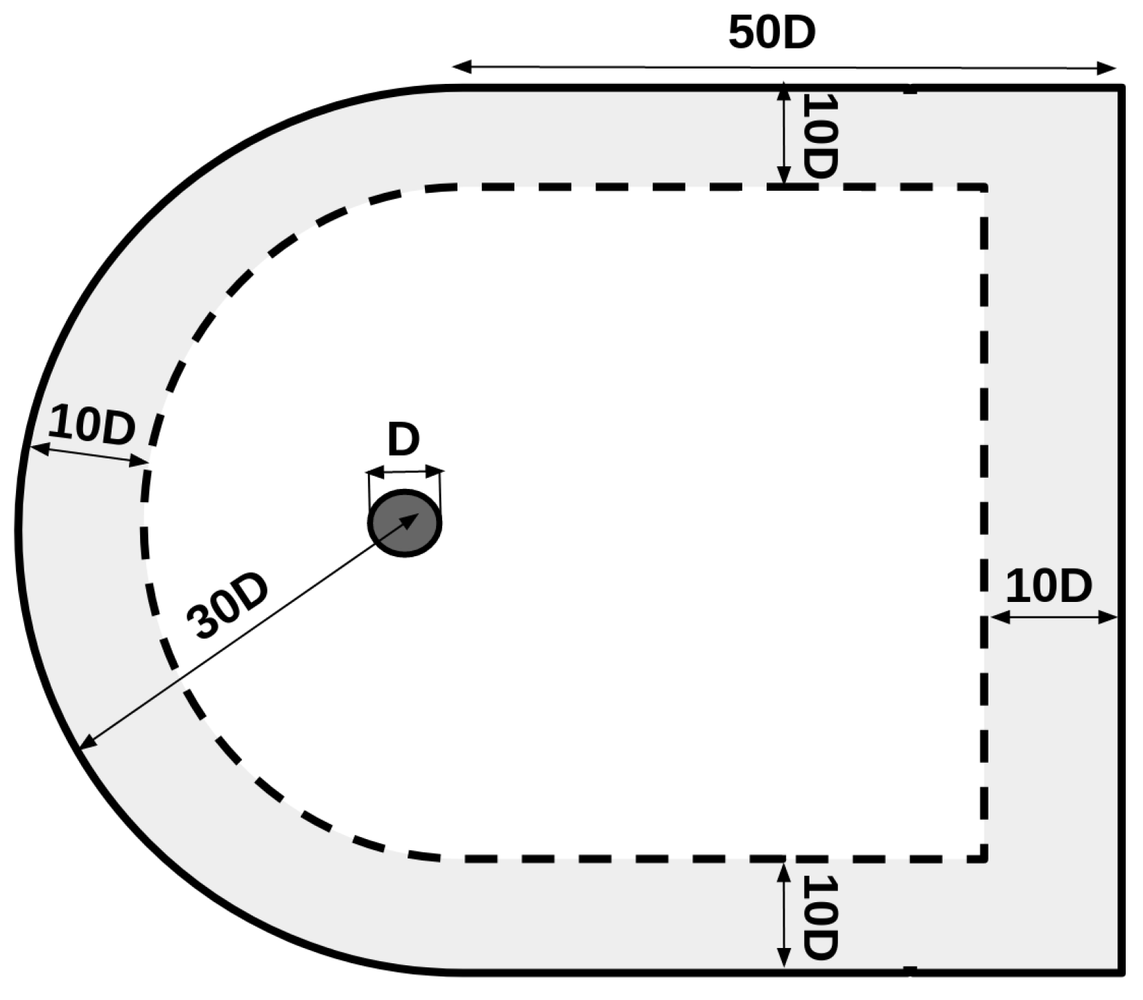
2.3. Far-Field Noise Prediction

The computation of the far-field noise was carried out using the Ffowcs Williams–Hawkings (FWH) acoustic analogy [20], which consists of an exact rearrangement of the Navier–Stokes equations into the form of an inhomogeneous wave equation. By using the theory of distributions [52], the pressure perturbations can be expressed as a function of quadrupole sound sources in the volume surrounding the body and monopole and dipole sound sources on the body surface (f) [21]:

$${\square }^2\left(p^{\prime }(\mathbf{x},t)\right)H\left(f\right)=\frac{\partial }{\partial t}\left[{\rho }_0{u}_i{n}_i\delta \left(f\right)\right]-\frac{\partial }{\partial x_i}\left[p_{ij}{n}_j\delta \left(f\right)\right]+\frac{{\partial }^2{T}_{ij}H\left(f\right)}{\partial x_i\partial x_j}$$

(7)

where ${\square }^2$ is the d’Alembert operator,

$${\square }^2=\frac{{\partial }^2}{\partial x_i^2}-\frac{1}{a_0^2}\frac{{\partial }^2}{\partial t^2}$$

(8)

$p^{\prime }(\mathbf{x},t)$ accounts for the acoustic pressure evaluated at the microphone point $\mathbf{x}$ and at the receiving time t. $H\left(f\right)$ is the Heaviside step function (the Heaviside function, or unit step function, is a step function that has a value of 0 for negative arguments and 1 for positive arguments) and $\delta \left(f\right)$ is the Dirac delta function (the Dirac delta distribution, or unit impulse, is a generalized function that has a value of 0 everywhere except at 0; its integral over the entire real line is equal to 1), which were used to denote whether the terms were to be evaluated on the body surface or in the external volume. $n_i=\mid \nabla f\mid$ are the components of the outward unit normal vector, and the Lighthill stress tensor is represented by

$$T_{ij}=\rho u_i{u}_j+p_{ij}-a_0^2\rho {\delta }_{ij}$$

(9)

The volume evaluation of the Lighthill stress tensor, which accounts for the quadrupole sources, is by far the most expensive term of the Ffowcs–Williams Hawkings analogy and it is usually neglected for low-Mach-number flows as their power relative to the dipole sources increases with the square of the Mach number [15].

For those applications where quadrupoles are relevant (see, for instance, the studies on the noise radiated by wakes of subsonic flows by Wolf et al. [53,54]), Di Francescantonio [55] proposed changing f to a permeable moving surface moving at a velocity $v_i=0$ that encloses all the volumetric sources producing non-negligible noise instead of using the body surface.

Equation (7) can then be rearranged to include the terms accounting for the evaluation of the noise sources in the permeable surface:

$${\square }^2\left(p^{\prime }(\mathbf{x},t)\right)H\left(f\right)=\frac{\partial }{\partial t}\left[Q_i{n}_i\delta \left(f\right)\right]-\frac{\partial }{\partial x_i}\left[L_{ij}{n}_j\delta \left(f\right)\right]+\frac{{\partial }^2{T}_{ij}H\left(f\right)}{\partial x_i\partial x_j}$$

(10)

with

$$\begin{array}{cc}\hfill Q_i& =\rho \left(u_i-v_i\right)+{\rho }_0{v}_i\hfill \\ \hfill L_{ij}& =\rho u_i\left(u_j-v_j\right)+p_{ij}\hfill \end{array}$$

(11)

After changing the evaluation surface, the term

$$\frac{{\partial }^2{T}_{ij}H\left(f\right)}{\partial x_i\partial x_j}$$

(12)

can be neglected as its contribution is already included in the terms evaluated on the permeable surface. Hence, the total acoustic pressure can be computed with the sum of the thickness and loading contributions,

$$p^{\prime }(\mathbf{x},t)=p_{\mathrm{T}}^{\prime }(\mathbf{x},t)+p_{\mathrm{L}}^{\prime }(\mathbf{x},t)$$

(13)

for which we have

$$\begin{array}{cc}\hfill 4\pi p_t^{\prime }(\mathbf{x},t)=& \frac{\partial }{\partial t}{\int }_{f=0}\frac{Q_i(\mathbf{y},\tau )n_i}{4\pi r}\mathrm{d}S\hfill \\ \hfill 4\pi p_l^{\prime }(\mathbf{x},t)=& -\frac{\partial }{\partial x_i}{\int }_{f=0}\frac{L_{ij}(\mathbf{y},\tau )n_j}{4\pi r}\mathrm{d}S\hfill \end{array}$$

(14)

with $Q_i$ and $L_{ij}$ evaluated at the source point $\mathbf{y}$ and at the emission time $\tau$. The relationship between the emission and receiving time is given by $\tau =t-r/a_0$, where r is the distance between the source and the microphone points and $a_0$ represents the free-stream speed of sound waves.

This formulation has been extended by Najafi-Yazdi et al. [56], who particularized the formulation for moving sources in uniformly moving media (also known as FWH formulation 1C), taking into account the presence of a mean flow. Furthermore, they also particularized formulation 1C for the wind tunnel scenario where the source and the observer are static and converted all spatial derivatives to time derivatives to make the equation more suitable for numerical integration:

$$4\pi p_T^{\prime }={\int }_{f=0}{\left[\left(1-M_0\right)\frac{{\dot{Q}}_i{n}_i}{r^{\ast }}-U_0\frac{{\tilde{r}}_1^{\ast }{Q}_i{n}_i}{r^{{\ast }^2}}\right]}_{\tau }dS$$

(15)

$$4\pi p_L^{\prime }={\int }_{f=0}{\left[\frac{1}{a_0}\frac{{\dot{L}}_{ij}{n}_j{\tilde{r}}_i}{r^{\ast }}+\frac{L_{ij}{n}_j{\tilde{r}}_i^{\ast }}{r^{{\ast }^2}}\right]}_{\tau }dS$$

(16)

where the ∗, ′ and · superscripts indicate a wind-tunnel quantity, a perturbation quantity (e.g., ${\rho }^{\prime }=\rho -{\rho }_0$) and a source-temporal derivative. $U_0$ and $M_0$ are the wind-tunnel velocity and Mach number, r is the distance from the source on the data surface to the observer and ${\tilde{r}}_i$ is the radiation vector components (i.e., the vector pointing from the source to the observer).

The terms containing ${r^{\ast }}^2$ vanish quickly in the far field as $r^{\ast }\to \infty$ and thus they are significant only in the near-field region. It should be noted that the amplitude of the thickness term’s contribution to the far-field noise decreases with an increasing mean flow Mach number. Therefore, loading noise becomes the dominant source term in flows with high Mach numbers [56].

Figure 2 shows the permeable surface used in the present work and how it encloses all the vortical structures. There are several approaches to avoid the spurious sound sources that appear due to the effect of the permeable surface location; for instance, Zhou et al. [57] reported that they can be suppressed using a correction model. In this work, the surface was defined following a similar criterion to the one used by Yao et al. [23]. It was designed considering that it has to enclose all the non-dimensionless vorticity isocontours larger than 4.

The surface must be far enough from the wake so that no spurious sources cross its faces and as close as possible to the source to avoid dissipation by mesh coarsening and numerical methods [58]. If designed appropriately, the surface can be incomplete in case the volume sources must go across it. Ricciardi et al. [59] proved that results are still accurate if it is necessary to open this gap to avoid truncating the sound sources.

As a result, far-field acoustic computation can be reduced to solving two surface integrals. This approach is commonly used due to its lower computational cost and robustness, and it is valid provided that the surface moves with a subsonic regime.

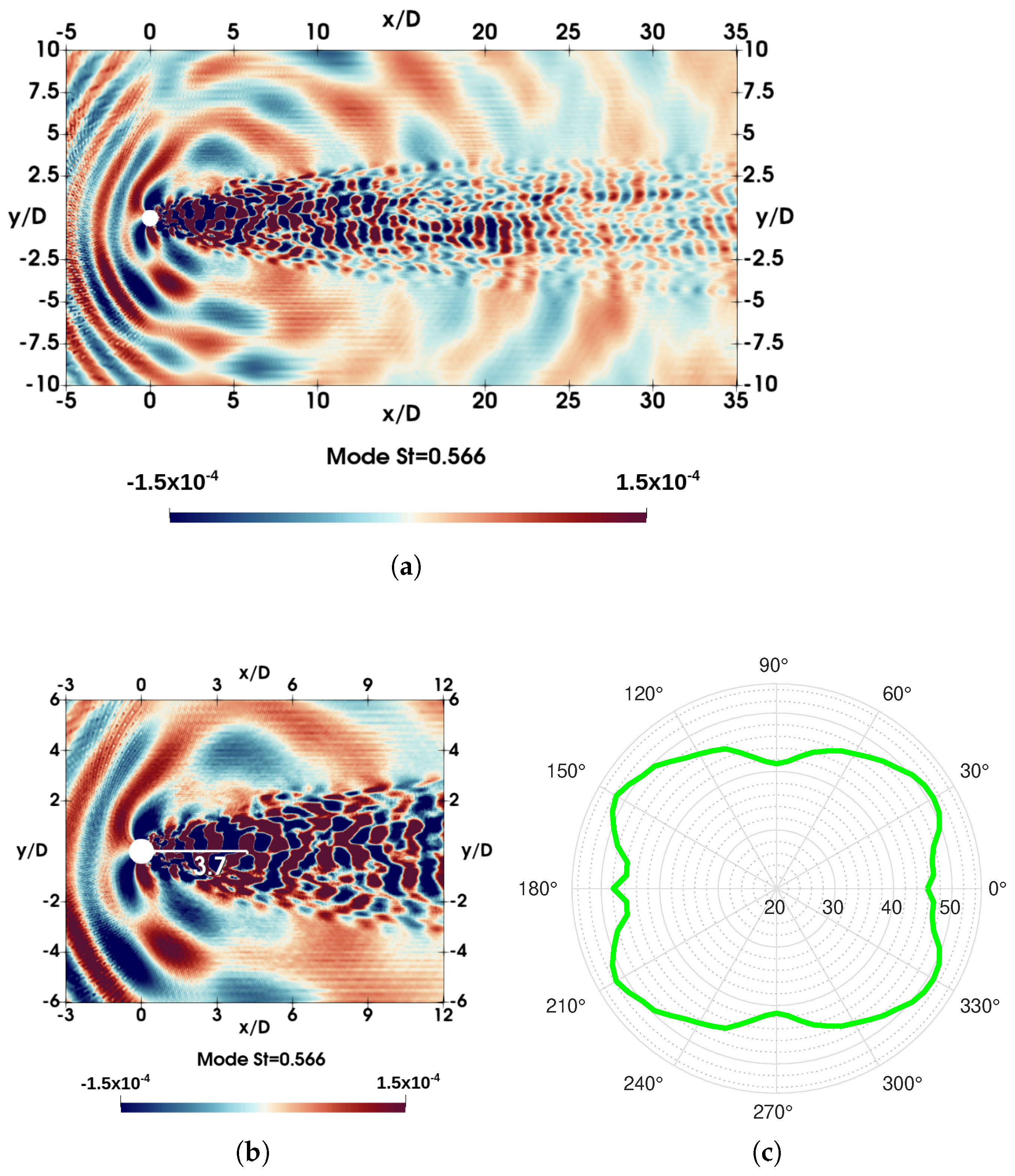
2.4. Dynamic Mode Decomposition (DMD)

Dynamic mode decomposition (DMD) is a frequency-based modal decomposition introduced by Schmid [41]. It arose from the need for snapshot-based decomposition that does not rank the flow structures according to their energy. DMD modes can be interpreted as structures with a linear tangent approximation to the underlying flow and describe fluid elements that have dominant dynamic behavior inside the captured data. The fact that the modes extracted from DMD are part of a dynamic system implies that they are not a spatial correlation with a time signal but a coherent structure with an associated frequency, amplitude and damping ratio.

DMD is a data-based procedure and ignores any other information for the system besides the flow-field data, which have to be presented in a snapshot sequence given by the matrix ${\mathcal{D}}_1^N$:

$${\mathcal{D}}_1^N=\left[d_1,d_2,d_3,\dots ,d_N\right]$$

(17)

where $d_i$ stands for the ith flow field. Following the original formulation from Schmid [41], the first step is to assume that there exists a linear mapping A that connects the field $d_i$ to the next field $d_{i+1}$:

$$d_{i+1}=A{d}_i$$

(18)

If A is assumed as constant, it is possible to formulate the sequence of flow fields as a Krylov sequence:

$${\mathcal{D}}_1^N=\left[d_1,A{d}_1,A^2{d}_1,\dots ,A^{N-1}{d}_1\right]$$

(19)

In this work, A was computed following the algorithm presented by Tu et al. [60], and then the characteristics of the dynamical process described by A were extracted with the eigenvalue decomposition. As the final step of the dynamic mode decomposition, the amplitude of each mode was computed with the method introduced by Jovanovic et al. [61].

3. Results

3.1. Flow Field Validation

The fluid flow validation was undertaken by comparing the obtained results against available data from the literature. Despite there not being any other study of the same conditions, multiple works have studied the aerodynamics of a cylinder with the subcritical regime under the incompressibility hypothesis [62,63,64] or with $M=0.5$ at higher Reynolds numbers [65]. In order to ensure statistical convergence, after discarding the initial transient, all the results were time-averaged along 400TU and spanwise-averaged along the 66 planes of the numerical grid.

In

Table 1. Aerodynamic flow quantities: non-dimensional vortex shedding frequency, average drag coefficient, RMS lift coefficient and mean recirculation length $Lc/D$. If the Mach number is not indicated, it is referred to incompressible flow conditions.

Case	${\mathit{St}}_{\mathit{VS}}$	$\overline{{\mathit{C}}_{\mathit{d}}}$	${\mathit{C}}_{\mathit{L}}^{\mathit{rms}}$	${\mathit{L}}_{\mathit{c}}/\mathit{D}$
Abrahamsen et al. ($R{e}_D=1.31\times {10}^4$, LES) [64]	—	—	—	0.712
Dong and Karniadakis ($R{e}_D=1\times {10}^4$, DNS) [63]	0.203	1.143	—	0.820
Wieselsberger (exp.) [68]	—	1.143	—	—
Gopalkrishnan (exp.) [69]	0.193	1.186	—	—
Norberg ($R{e}_D=8.1\times {10}^3$, exp.) [70]	—	—	—	1.022
Norberg ($R{e}_D=8.1\times {10}^3$, exp.) [62]	0.202	—	—	—
Khalighi et al. ($R{e}_D=1\times {10}^4$, $M=0.2$, LES) [24]	0.192	1.290	0.630	0.680
O. Rodríguez ($R{e}_D=8\times {10}^4$, $M=0.55$, exp.) [71]	—	1.455	—	—
Murthy and Rose ($R{e}_D=8.3\times {10}^4$, $M=0.4$, exp.) [67]	0.183	1.430	—	—
Present LES	0.194	1.388	0.487	0.840

, a summary of the available results from the literature for the Strouhal number, $St=f_{VS}D/U_0$; the average drag coefficient, $\overline{C_D}$; the root mean square value of the lift coefficient, $C_L^{rms}$; and the recirculation length, $L_c/D$, is presented. In general, the average flow parameters obtained were within the ranges of those reported in the literature. It should be pointed out that the drag coefficient, and thus the recirculation length, is affected by compressibility effects, as reported in the literature (see, for instance, the works by Welsh [66] and Murthy and Rose [67]), whereas almost no dependence for the non-dimensional vortex shedding frequency has been observed [67].

Additionally, in Figure 3, the spectrum of the pressure fluctuations of a numerical probe located in the shear layer at $x/D=0.30$ and $y/D=0.55$ is depicted. The energy spectrum exhibits a narrow-band peak located at $St=0.194$, which matches the vortex shedding frequency, and a broad-band peak centered at $St=1.972$, which corresponds with the passage of the Kelvin–Helmholtz (KH) instabilities. If the ratio of this frequency to that of the vortex shedding is evaluated, it yields $f_{KH}/f_{VS}=10.16$, in good agreement with the value predicted by Prasad and Williamson correlation [72]: $f_{KH}/f_{VS}=0.0235R{e}^{0.67}=11.24$.

To conclude the fluid flow validation, Figure 4 compares the surface pressure coefficient ($C_P=(p-p_0)/\left(0.5{\rho }_0{U}_0\right)$) along the cylinder surface with results from the literature under comparable conditions. As the flow is in the subcritical regime, despite the differences in Reynolds number, the pressure distribution shows very good agreement with the experimental results obtained by Gowen and Perkins [65] at the same Mach number. Moreover, a fair agreement can be observed when comparing with the results for the incompressible flow (see the work by Norberg [62] and Dong and Karniadakis [63]), although a small deviation in the base pressure zone can be observed. These differences were expected owing to the increase in the drag coefficient with the Mach number (see, for instance, the work by Murthy and Rose [67]).

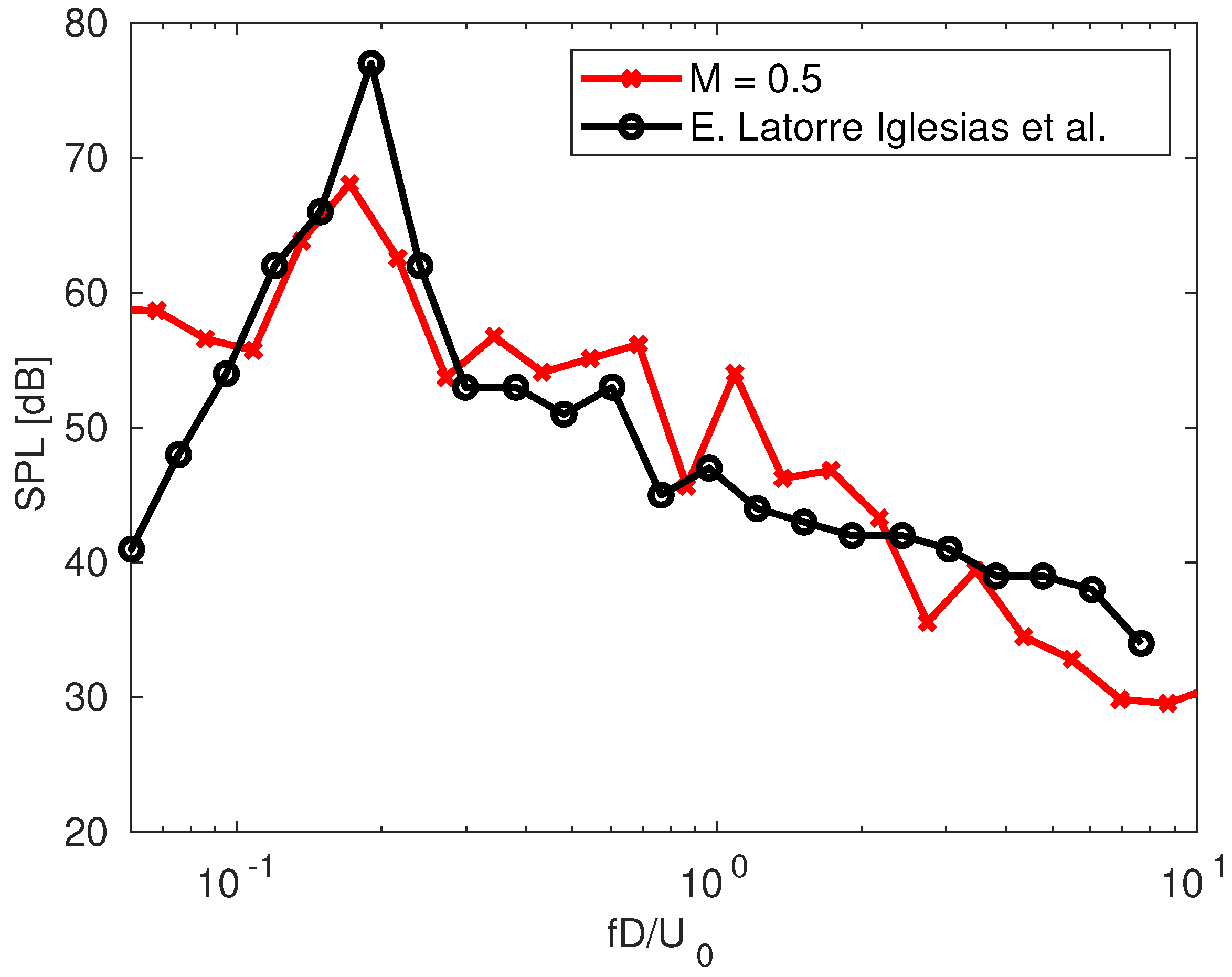
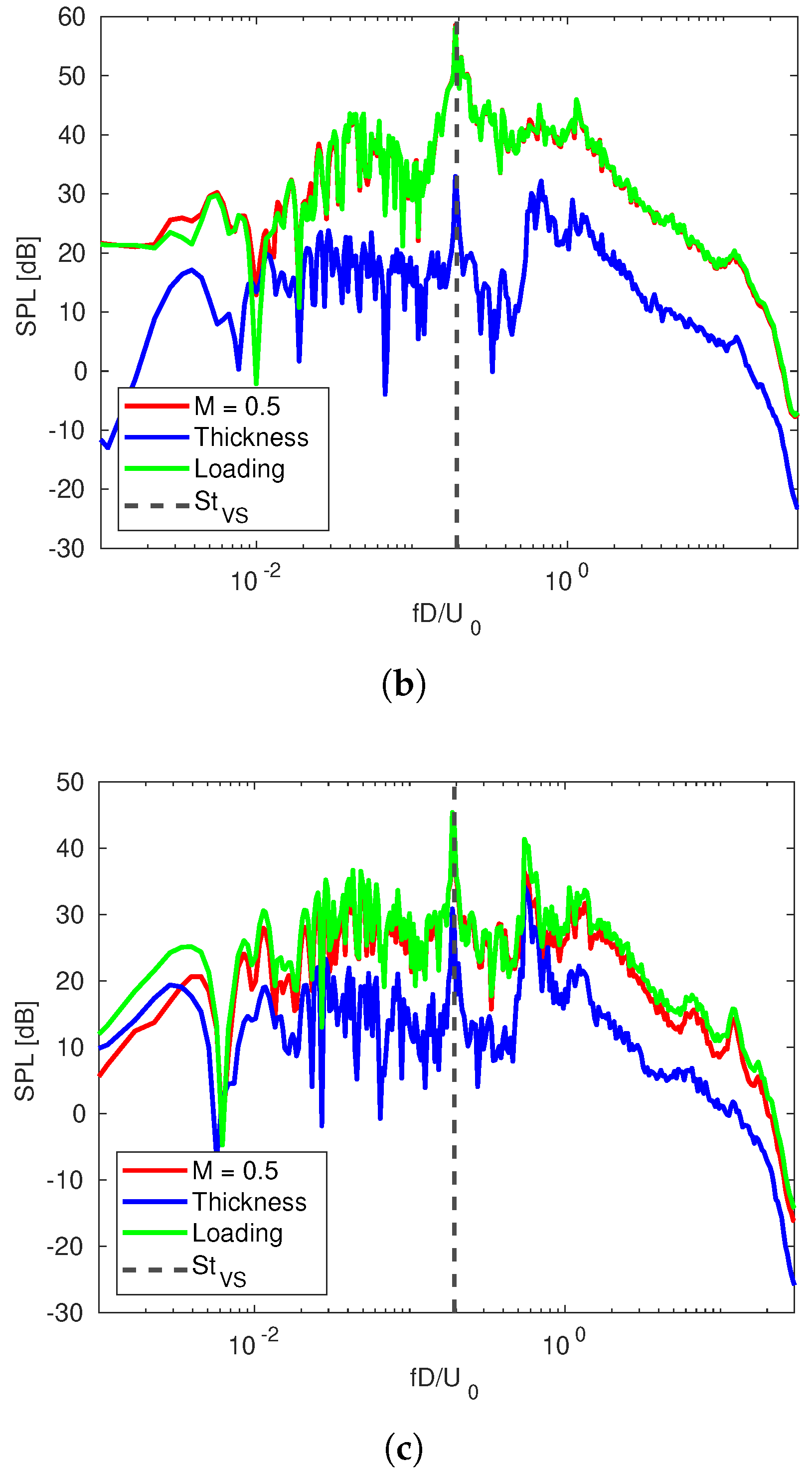
3.2. Noise Field Results

In Figure 5, a comparison between the acoustic pressure for an observer located at a distance $r/D=100$ in the cross-stream direction and the results obtained by E. Latorre Iglesias et al. [34] for an observer located in the same direction at $r/D=116$ is presented. The experiments undertaken by E. Latorre Iglesias et al. were conducted at $Re=2.59\times {10}^4$ and at a Mach number of $M=0.09$. In general, a rather good agreement can be observed, and the main difference is in the magnitude of the peak value of the aeolian tone. This difference can be attributed to the different flow conditions, especially the different Mach numbers, between the present computations and the experiments.

Figure 6 shows an instantaneous snapshot of the wake and its radiated noise. The wake is dominated by the von Kármán vortex street and its structures are illustrated using the Q criterion isocontours [73] colored with the spanwise vorticity. The dilatation field, defined as $\nabla ·\left(\rho \mathbf{u}\right)$, illustrates the sound wave propagation and shows that all the noise is generated in the vicinity of the cylinder.

Dynamic mode decomposition (DMD) [41] was applied to the pressure fluctuations in order to identify the noise sources. To do so, 370 snapshots spaced with a $dt=0.166$ TU along a total timespan of 61.5 TU were used. Figure 7a shows the plot of the amplitude of the DMD modes against their non-dimensional frequency. The mode with the highest amplitude was the one that took place at the vortex shedding frequency and the rest of the amplitudes were scaled according to this value. The spectra of the lift and drag forces (Figure 7b) indicate three distinct frequency domains that correspond to the significance of the respective force fluctuations. The lift fluctuations dominate at frequencies lower than $fD/U_0<0.32$. On the other hand, at $0.32<fD/U_0<0.45$, the fluctuations of the drag force have more relevance in the flow, and finally, at $fD/U_0>0.45$, neither force exhibits relevant fluctuations anymore. This yielded a division of the DMD modes into three different groups (colored in red, blue and green in Figure 7a) depending on the most relevant force fluctuation.

Figure 8a shows the spatial correlation of 1 of the 26 modes with a frequency lower than ($fD/U_0<0.32$). In particular, it depicts the mode at the vortex shedding frequency ($f_{VS}D/U_0=0.194$). All the modes in this group highlight the cross-stream pressure fluctuations in the wake of the cylinder and the sound waves that they generate. Figure 8b provides a closer look of the wave generation area of the vortex shedding mode to show the position of the noise source. In this mode, the center of the sound waves is located at $x/D=1.25$ ($0.75D$ behind the cylinder).

Figure 8c plots the evolution of the DMD mode in the streamwise direction using a horizontal line at $y/D=0$ going from $x/D=-0.5$ to $x/D=-12$ (colored in black). The plot in the cross-stream direction was produced using two vertical lines at $x/D=1.25$ going from $y/D=0$ to $y/D=-15$ (colored in red) and to $y/D=15$ (colored in blue). This plot makes evident that the sound waves mostly radiated in the direction perpendicular to the flow with a wavelength of $\lambda =8.31D$ and that the waves propagated from the top and bottom side had a phase-shift of $\varphi =\pi /2$.

The rest of the modes in the group had a very similar pattern in the wake pressure fluctuations; however, the wavelength of the sound changed according to the frequency of the mode. Moreover, the position of the center of the noise source was slightly different from the one depicted in Figure 8b, but it never went behind the endpoint of the recirculation bubble ($x/D=1.34$). In all cases, the waves radiated in the direction perpendicular to the flow with a phase shift of $\varphi =\pi /2$.

To see how these modes affect the far-field noise, the acoustic pressure was computed for a circular array of 72 equispaced virtual microphones arranged concentrically with the cylinder at a radius of $r=100D$. Figure 9 shows the OASPL integrated in the range of frequencies of this set of modes ($0<fD/U_0<0.32$). The resulting directivity pattern was dipole-oriented in the cross-stream direction and comparable to the one obtained by Liu et al. [32] at the same distance for an incompressible flow at $R{e}_D=26,700$. Considering that dipoles are characteristic of momentum fluctuations, that all the modes in this group took place at frequencies where the lift force fluctuations had a dominant effect and that the waves were generated by cross-stream fluctuations, it can be confirmed that Figure 8a shows the noise source related to the lift force fluctuations.

Figure 10a shows the mode at the first harmonic of the vortex shedding frequency, $fD/U_0=2S{t}_{VS}=0.389$. This spatial correlation is used to illustrate all the 12 modes that had a frequency in the range $0.32<fD/U_0<0.45$, where the drag force fluctuations had a dominant effect. In all the modes in this range, the wake was driven by the streamwise pressure fluctuations and the sound waves that they generated. As shown in Figure 10b, the center of the soundwaves in this mode was located at $x/D=3.7$ ($3.2D$ behind the cylinder), further downstream than the modes linked to the lift force fluctuations.

Figure 10c shows the resulting line plots in the streamwise and cross-stream directions using the same criteria as in Figure 8c. In this case, the origin of the vertical lines was shifted to $x/D=3.7$ to make it coincide with the center of the noise source. The main difference compared to the modes linked to the lift fluctuations was the appearance of sound waves in the streamwise direction at a wavelength of $\lambda =2.56D$. Regarding the cross-stream direction, the wavelength of this mode was reduced to nearly half of the one in the vortex shedding mode, $\lambda =4.22D$, and the waves propagated to the top of the cylinder were in phase with the bottom ones.

Although the radiation intensity was quite similar in the two directions, the different wavelengths led to a dipole distribution in the far field (Figure 11). It can thus be concluded that the noise source in Figure 10a and the rest of the modes inside the range $0.32<fD/U_0<0.45$ were related to the drag force fluctuations. Additionally, Figure 11 compares the relevance of the drag dipole with the lift dipole presented in Figure 9, showing that the drag dipole only has a small effect in the streamwise direction.

The 320 modes that occurred at frequencies higher than $fD/U_0>0.45$ were no longer linked with force fluctuations. Hence, their spatial correlations did not present a common pattern in the wake fluctuations as none of the modes contained features related to the streamwise or cross-stream pressure fluctuations. Figure 12a represents the mode with a higher amplitude in that region at a frequency of $fD/U_0=0.566$. Figure 12b provides a closer look at the sound wave generation area of the mode to show that the center of the waves was located at $x/D=4.2$, $3.7D$ behind the cylinder. The directivity pattern at $r/D=100$ of this frequency (Figure 12c) shows that this mode emitted sound to the far field as a quadrupole source. The points with a higher sound pressure level were the ones located at ${30}^{\circ }$, ${150}^{\circ }$, ${210}^{\circ }$ and ${330}^{\circ }$. The observers in the cross-stream direction were the ones that received a lower sound signal, followed by the ones aligned with the direction of the flow.

This was an expected result because the momentum fluctuations were really weak at $fD/U_0>0.45$, and only the shear fluctuations, which led to a quadrupole distribution, could be responsible for sound generation. Although the rest of the modes at this range of frequencies might present significant differences in the wake pressure correlations, the individual directivity pattern for each frequency in the far field results in a quadrupole. Its shape, intensity and orientation depend on the emission point of the sound waves, the wavelengths, the radiation direction and the phase shifts of each of the modes.

Figure 13 shows the OASPL of the addition of the lift and drag dipoles ($fD/U_0<0.45$), the OASPL of the modes that led to quadrupole noise sources ($fD/U_0>0.45$) and the global OASPL integrated in the range $\left[0.01<fD/U_0<10\right]$. The quadrupole sources had a small effect in the cross-stream direction but gained intensity as the observer came closer to the parallel direction of the flow. All these results were compared with the directivity pattern obtained for an incompressible flow by Liu et al. [32], showing that the compressibility effects, which mainly lead to the appearance of quadrupole sources, are higher in the streamwise direction than in the cross-stream one. It should also be mentioned that the directivity pattern of the global OASPL showed that the sound intensity radiated in the streamwise direction was only 5 dB lower than the intensity in the perpendicular direction. This yielded an overall directivity pattern that was close to being a monopole due to the superposition of the lift and drag dipoles together with the quadrupoles.

The final analysis of the far-field sound radiation was undertaken with the sound pressure level (SPL) spectra at the observers in the streamwise and cross-stream directions (Figure 14). The spectra of the three observers presented a narrow band peak at the vortex shedding frequency as it was the most relevant tone for all of them. However, its value was much higher at the cross-stream observer (up to 62 dB) than at the streamwise one, where it only reached 46 dB. None of the observers presented a significant peak at the second harmonic of the vortex shedding frequency nor in the range where the drag force fluctuations dominated ($0.32<fD/U_0<0.45$). This observation confirmed that these fluctuations had minimal impact on the far-field sound. The streamwise observers exhibited a broad peak within the frequency range where the quadrupole sources had been identified. This clearly demonstrated their significance in the streamwise direction.

In addition to the total sound pressure level values, Figure 14 also presents the spectra for the thickness (Equation (15)) and loading (Equation (16)) terms of the 1C formulation of the Ffowcs Williams–Hawkings analogy. The thickness term accounts for the contribution of monopoles, and their effect was comparable to the loading term in the high-frequency wide-band peak present at the observers in the streamwise direction.

4. Summary

The present study investigated the noise generated by the flow around a cylinder in the subcritical regime at $R{e}_D=1\times {10}^4$ and a subsonic Mach number of $M=0.5$. Large-eddy simulations of the compressible Navier–Stokes equations were employed to resolve the flow field and analyze near-field noise generation directly. The flow field was validated with experimental and numerical studies performed under similar conditions and the noise field results exhibited good agreement with the studies under similar conditions by E. Latorre Iglesias et al. [34] and Liu et al. [32].

The dynamic mode decomposition [41] of the pressure field was used to detect the noise sources in the near field and the wind-tunnel version of formulation 1C of the Ffowcs Williams–Hawkings analogy [56] was used to determine the effect of each of the sources in the far field at a distance of $r/D=100$. The DMD modes were grouped in three different frequency ranges depending on which of the forces had a more dominant fluctuation. Lift fluctuations were more relevant at $fD/U_0<0.32$, the drag fluctuations dominated at $0.32<fD/U_0<0.45$ and neither force had relevant fluctuations beyond $fD/U_0>0.45$.

The sound waves of the modes in the first range radiated in the cross-stream direction with a phase shift of $\varphi =\pi /2$. They generated a dipole distribution in the far field, which was comparable to the OASPL of the incompressible flow studied by Liu et al. [32]. The most relevant mode in the range was the one at the vortex shedding frequency and all the sound radiated by the 26 modes was linked to the lift fluctuations.

The 12 modes in the second frequency range were linked to the drag fluctuations. In this case, the waves radiated in all directions but at different wavelengths in the streamwise ($\lambda =2.56$) and the cross-stream directions ($\lambda =4.22D$). This led to a dipole directivity pattern in the far field. When compared with the dipole generated by the lift sound sources, its contribution was only relevant to the observers located parallel to the flow.

The modes at the frequencies where the momentum fluctuations were not relevant ($fD/U_0>0.45$) led to quadrupole sources of different shapes, intensities and orientations. The integral of the sound pressure level in this range of frequencies, however, showed that its effect was remarkable in far-field observers located in the streamwise direction, while it had a small impact in the direction perpendicular to the flow.

The OASPL of the superposition of the three types of sources identified led to a directivity pattern that was close to being a monopole, as the sound pressure level in the streamwise direction was only 5 dB lower than the sound radiated in the cross-stream one.

The spectral analysis of the sound pressure level (SPL) computed at the microphones located at $0^{\circ }$, ${90}^{\circ }$ and ${180}^{\circ }$ revealed a dominant peak at the non-dimensional vortex shedding frequency ($fD/U_0=0.194$), the highest value (62 dB) being at the observer placed at ${90}^{\circ }$. This related the peak with the dipole contribution of the lift force fluctuations. Moreover, a wide-band peak that extended from $fD/U_0=0.566$ to $fD/U_0=1.987$ was observed at the microphones located at $0^{\circ }$ and ${180}^{\circ }$. This peak accounted for the influence of quadrupole sources radiating noise in the direction parallel to the flow. The contributions of the thickness and loading terms illustrated that the monopole contributions were less important than the addition of the dipole and quadrupole sources, especially at ${90}^{\circ }$, where they barely had an impact.

All in all, this work helps to identify how the aerodynamic noise radiated by a cylinder changes with the increase in the Mach number inside the subsonic regime by shedding light on the frequency, pattern and intensity of each of the noise sources in the far field, as well as the originating pressure fluctuations in the near field.

References

1. Hanning, C.D.; Evans, A.D. Wind turbine noise. BMJ Br. Med. J. 2012, 344. [Google Scholar] [CrossRef] [PubMed]
2. Van den Berg, F. Wind turbine noise: An overview of acoustical performance and effects on residents. Proc. Acoust. 2013. Available online: http://docs.wind-watch.org/AAS-2013-p108-van-den-Berg.pdf (accessed on 1 February 2022).
3. Deshmukh, S.; Bhattacharya, S.; Jain, A.; Paul, A.R. Wind turbine noise and its mitigation techniques: A review. Energy Procedia 2019, 160, 633–644. [Google Scholar] [CrossRef]
4. Fritschi, L.; Brown, L.; Kim, R.; Schwela, D.H.; Kephalopolous, S. Burden of Disease from Environmental Noise: Quantification of Healthy Life Years Lost in Europe; World Health Organization: Geneva, Switzerland, 2011. [Google Scholar]
5. Eriksson, C.; Pershagen, G.; Nilsson, M. Biological Mechanisms Related to Cardiovascular and Metabolic Effects by Environmental Noise; Technical Documents; WHO: Geneva, Switzerland, 2018; Volume 3, p. 13. [Google Scholar]
6. Knörzer, D.; Szodruch, J. (Eds.) Flightpath 2050: Europe’s vision for aeronautics. In Innovation for Sustainable Aviation in a Global Environment: Proceedings of the Sixth European Aeronautics Days, Madrid; IOS Press: Amsterdam, The Netherlands, 2012; Volume 30. [Google Scholar]
7. Xiao-Ming, T.; Zhi-Gang, Y.; Xi-Ming, T.; Xiao-Long, W.; Jie, Z. Vortex structures and aeroacoustic performance of the flow field of the pantograph. J. Sound Vib. 2018, 432, 17–32. [Google Scholar] [CrossRef]
8. Zhang, Y.; Zhang, J.; Li, T.; Zhang, L. Investigation of the aeroacoustic behavior and aerodynamic noise of a high-speed train pantograph. Sci. China Technol. Sci. 2017, 60, 561–575. [Google Scholar] [CrossRef]
9. Ikeda, M.; Mitsumoji, T. Evaluation method of low-frequency aeroacoustic noise source structure generated by Shinkansen pantograph. Q. Rep. RTRI 2008, 49, 184–190. [Google Scholar] [CrossRef]
10. Keating, A.; Dethioux, P.; Satti, R.; Noelting, S.; Louis, J.; Van de Ven, T.; Vieito, R. Computational aeroacoustics validation and analysis of a nose landing gear. In Proceedings of the 15th AIAA/CEAS Aeroacoustics Conference (30th AIAA Aeroacoustics Conference), Miami, FL, USA, 11–13 May 2009; p. 3154. [Google Scholar]
11. Lockard, D.; Khorrami, M.; Li, F. Aeroacoustic analysis of a simplified landing gear. In Proceedings of the 9th AIAA/CEAS Aeroacoustics Conference and Exhibit, Hilton Head, SC, USA, 12–14 May 2003; p. 3111. [Google Scholar]
12. Redonnet, S.; Khelil, S.B.; Bulté, J.; Cunha, G. Numerical characterization of landing gear aeroacoustics using advanced simulation and analysis techniques. J. Sound Vib. 2017, 403, 214–233. [Google Scholar] [CrossRef]
13. Williamson, C.H. Vortex dynamics in the cylinder wake. Annu. Rev. Fluid Mech. 1996, 28, 477–539. [Google Scholar] [CrossRef]
14. Leehey, P.; Hanson, C. Aeolian tones associated with resonant vibration. J. Sound Vib. 1970, 13, 465–483. [Google Scholar] [CrossRef]
15. Curle, N. The influence of solid boundaries upon aerodynamic sound. In Proceedings of the Royal Society of London. Series A. Mathematical and Physical Sciences; The Royal Society: London, UK, 1995; Volume 231, pp. 505–514. [Google Scholar]
16. Phillips, O.M. The intensity of Aeolian tones. J. Fluid Mech. 1956, 1, 607–624. [Google Scholar] [CrossRef]
17. Etkin, B.; Korbacher, G.K.; Keefe, R.T. Acoustic Radiation from a Stationary Cylinder in a Fluid Stream (Aeolian Tones). J. Acoust. Soc. Am. 1957, 29, 30–36. [Google Scholar] [CrossRef]
18. Wagner, C.; Hüttl, T.; Sagaut, P. Large-Eddy Simulation for Acoustics; Cambridge Aerospace Series; Cambridge University Press: Cambridge, UK, 2007; Volume 20. [Google Scholar] [CrossRef]
19. Lighthill, M.J. On sound generated aerodynamically I. General theory. Proc. R. Soc. London Ser. A Math. Phys. Sci. 1952, 211, 564–587. [Google Scholar]
20. Williams, J.F.; Hawkings, D.L. Sound generation by turbulence and surfaces in arbitrary motion. In Philosophical Transactions for the Royal Society of London. Series A Mathematical and Physical Sciences; The Royal Society: London, UK, 1969; pp. 321–342. [Google Scholar]
21. Brentner, K.S.; Farassat, F. Modeling aerodynamically generated sound of helicopter rotors. Prog. Aerosp. Sci. 2003, 39, 83–120. [Google Scholar] [CrossRef]
22. Cianferra, M.; Ianniello, S.; Armenio, V. Assessment of methodologies for the solution of the Ffowcs Williams and Hawkings equation using LES of incompressible single-phase flow around a finite-size square cylinder. J. Sound Vib. 2019, 453, 1–24. [Google Scholar] [CrossRef]
23. Yao, H.D.; Davidson, L.; Eriksson, L.E. Noise radiated by low-Reynolds number flows past a hemisphere at Ma = 0.3. Phys. Fluids 2017, 29, 076102. [Google Scholar] [CrossRef]
24. Khalighi, Y.; Mani, A.; Ham, F.; Moin, P. Prediction of Sound Generated by Complex Flows at Low Mach Numbers. AIAA J. 2010, 48, 306–316. [Google Scholar] [CrossRef]
25. Cai, J.C.; Pan, J.; Kryzhanovskyi, A.; E, S.J. A numerical study of transient flow around a cylinder and aerodynamic sound radiation. Thermophys. Aeromechanics 2018, 25, 331–346. [Google Scholar] [CrossRef]
26. Alhawwary, M.; Wang, Z. Implementation of a FWH approach in a high-order LES tool for aeroacoustic noise predictions. In AIAA Scitech 2020 Forum; American Institute of Aeronautics and Astronautics: Reston, VA, USA, 2020; Volume 1. [Google Scholar] [CrossRef]
27. Shur, M.L.; Spalart, P.R.; Strelets, M.K. Noise prediction for increasingly complex jets. Part II: Applications. Int. J. Aeroacoustics 2005, 4, 247–266. [Google Scholar] [CrossRef]
28. Morris, P.J.; Long, L.N.; Scheidegger, T.E.; Boluriaan, S. Simulations of Supersonic Jet Noise. Int. J. Aeroacoustics 2002, 1, 17–41. [Google Scholar] [CrossRef]
29. Uzun, A.; Lyrintzis, A.S.; Blaisdell, G.A. Coupling of Integral Acoustics Methods with LES for Jet Noise Prediction. Int. J. Aeroacoustics 2004, 3, 297–346. [Google Scholar] [CrossRef]
30. Moreau, S. The third golden age of aeroacoustics. Phys. Fluids 2022, 34, 031301. [Google Scholar] [CrossRef]
31. Cox, J.S.; Brentner, K.S.; Rumsey, C.L. Computation of vortex shedding and radiated sound for a circular cylinder: Subcritical to transcritical Reynolds numbers. Theor. Comput. Fluid Dyn. 1998, 12, 233–253. [Google Scholar] [CrossRef]
32. Liu, X.; Thompson, D.J.; Hu, Z. Numerical investigation of aerodynamic noise generated by circular cylinders in cross-flow at Reynolds numbers in the upper subcritical and critical regimes. Int. J. Aeroacoustics 2019, 18, 470–495. [Google Scholar] [CrossRef]
33. Orselli, R.; Meneghini, J.; Saltara, F. Two and three-dimensional simulation of sound generated by flow around a circular cylinder. In Proceedings of the 15th AIAA/CEAS Aeroacoustics Conference (30th AIAA Aeroacoustics Conference), Miami, FL, USA, 11–13 May 2009; p. 3270. [Google Scholar]
34. Iglesias, E.L.; Thompson, D.; Smith, M. Experimental study of the aerodynamic noise radiated by cylinders with different cross-sections and yaw angles. J. Sound Vib. 2016, 361, 108–129. [Google Scholar] [CrossRef]
35. Margnat, F.; da Silva Pinto, W.J.G.; Noûs, C. Cylinder aeroacoustics: Experimental study of the influence of cross-section shape on spanwise coherence length. Acta Acust. 2023, 7, 4. [Google Scholar] [CrossRef]
36. Sueki, T.; Ikeda, M.; Takaishi, T. Aerodynamic noise reduction using porous materials and their application to high-speed pantographs. Q. Rep. RTRI 2009, 50, 26–31. [Google Scholar] [CrossRef]
37. Geyer, T.F.; Sarradj, E. Circular cylinders with soft porous cover for flow noise reduction. Exp. Fluids 2016, 57, 30. [Google Scholar] [CrossRef]
38. Yu, P.; Xu, J.; Xiao, H.; Bai, J. Numerical Analysis of Aeroacoustic Characteristics around a Cylinder under Constant Amplitude Oscillation. Energies 2022, 15, 6507. [Google Scholar] [CrossRef]
39. Inoue, O.; Hatakeyama, N. Sound generation by a two-dimensional circular cylinder in a uniform flow. J. Fluid Mech. 2002, 471, 285–314. [Google Scholar] [CrossRef]
40. King, W.; Pfizenmaier, E. An experimental study of sound generated by flows around cylinders of different cross-section. J. Sound Vib. 2009, 328, 318–337. [Google Scholar] [CrossRef]
41. Schmid, P.J. Dynamic mode decomposition of numerical and experimental data. J. Fluid Mech. 2010, 656, 5–28. [Google Scholar] [CrossRef]
42. Favre, A.J. The Equations of Compressible Turbulent Gases. In Technical Report AD622097; Institut de Mecanique Statlstique de la Turbulence: Marseille, France, 1965. [Google Scholar]
43. Lehmkuhl, O.; Piomelli, U.; Houzeaux, G. On the extension of the integral length-scale approximation model to complex geometries. Int. J. Heat Fluid Flow 2019, 78, 108422. [Google Scholar] [CrossRef]
44. Rouhi, A.; Piomelli, U.; Geurts, B.J. Dynamic subfilter-scale stress model for large-eddy simulations. Phys. Rev. Fluids 2016, 1, 044401. [Google Scholar] [CrossRef]
45. Piomelli, U.; Rouhi, A.; Geurts, B.J. A grid-independent length scale for large-eddy simulations. J. Fluid Mech. 2015, 766, 499–527. [Google Scholar] [CrossRef]
46. Huang, P.; Coleman, G.; Bradshaw, P. Compressible turbulent channel flows: DNS results and modelling. J. Fluid Mech. 1995, 305, 185–218. [Google Scholar] [CrossRef]
47. Gasparino, L.; Muela, J.; Lehmkuhl, O. SOD2D Repository. Available online: https://gitlab.com/bsc_sod2d/sod2d_gitlab (accessed on 1 February 2022).
48. Guermond, J.L.; Pasquetti, R.; Popov, B. Entropy viscosity method for nonlinear conservation laws. J. Comput. Phys. 2011, 230, 4248–4267. [Google Scholar] [CrossRef]
49. Kennedy, C.A.; Gruber, A. Reduced aliasing formulations of the convective terms within the Navier–Stokes equations for a compressible fluid. J. Comput. Phys. 2008, 227, 1676–1700. [Google Scholar] [CrossRef]
50. Wasistho, B.; Geurts, B.J.; Kuerten, J.G. Simulation techniques for spatially evolving instabilities in compressible flow over a flat plate. Comput. Fluids 1997, 26, 713–739. [Google Scholar] [CrossRef]
51. Pope, S.B. Turbulent Flows; Cambridge University Press: Cambridge, MA, USA, 2000; Chapter 6. [Google Scholar]
52. Barros-Neto, J. An Introduction to the Theory of Distributions; M. Dekker: Weston, CT, USA, 1973; Volume 14. [Google Scholar]
53. Wolf, W.R.; Azevedo, J.L.F.; Lele, S.K. Convective effects and the role of quadrupole sources for aerofoil aeroacoustics. J. Fluid Mech. 2012, 708, 502–538. [Google Scholar] [CrossRef]
54. Wolf, W.R.; Cavalieri, A.V.G.; Backes, B.; Morsch-Flho, E.; Azevedo, J.L. Sound and Sources of Sound in a Model Problem with Wake Interaction. AIAA J. 2015, 53, 2588–2606. [Google Scholar] [CrossRef]
55. Di Francescantonio, P. A new boundary integral formulation for the prediction of sound radiation. J. Sound Vib. 1997, 202, 491–509. [Google Scholar] [CrossRef]
56. Najafi-Yazdi, A.; Brès, G.A.; Mongeau, L. An acoustic analogy formulation for moving sources in uniformly moving media. Proc. R. Soc. A Math. Phys. Eng. Sci. 2011, 467, 144–165. [Google Scholar] [CrossRef]
57. Zhou, Z.; Wang, H.; Wang, S.; He, G. Lighthill stress flux model for Ffowcs Williams–Hawkings integrals in frequency domain. AIAA J. 2021, 59, 4809–4814. [Google Scholar] [CrossRef]
58. Mitchell, B.E.; Lele, S.K.; Moin, P. Direct computation of the sound generated by vortex pairing in an axisymmetric jet. J. Fluid Mech. 1999, 383, 113–142. [Google Scholar] [CrossRef]
59. Ricciardi, T.R.; Wolf, W.R.; Spalart, P.R. On the Application of Incomplete Ffowcs Williams and Hawkings Surfaces for Aeroacoustic Predictions. AIAA J. 2022, 60, 1971–1977. [Google Scholar] [CrossRef]
60. Tu, J.H. Dynamic Mode Decomposition: Theory and Applications. Ph.D. Thesis, Princeton University, Princeton, NJ, USA, 2013. [Google Scholar]
61. Jovanović, M.R.; Schmid, P.J.; Nichols, J.W. Sparsity-promoting dynamic mode decomposition. Phys. Fluids 2014, 26. [Google Scholar] [CrossRef]
62. Norberg, C. Fluctuating lift on a circular cylinder: Review and new measurements. J. Fluids Struct. 2003, 17, 57–96. [Google Scholar] [CrossRef]
63. Dong, S.; Karniadakis, G.E. DNS of flow past a stationary and oscillating cylinder at Re = 10,000. J. Fluids Struct. 2005, 20, 519–531. [Google Scholar] [CrossRef]
64. Prsic, M.A.; Ong, M.C.; Pettersen, B.; Myrhaug, D. Large Eddy Simulations of flow around a smooth circular cylinder in a uniform current in the subcritical flow regime. Ocean. Eng. 2014, 77, 61–73. [Google Scholar] [CrossRef]
65. Gowen, F.E.; Perkins, E.W. Drag of circular cylinders for a wide range of Reynolds numbers and Mach numbers. In Technical Report NACA RM A52C20; NASA: Washington, DC, USA, 1952. [Google Scholar]
66. Welsh, C.J. The Drag of Finite-Length Cylinders Determined from Flight Tests at High Reynolds Numbers for a Mach Number Range from 0.5 to 1.3. In Technical Report NACA TN 2941; NASA: Washington, DC, USA, 1953. [Google Scholar]
67. Murthy, V.; Rose, W. Detailed measurements on a circular cylinder in cross flow. AIAA J. 1978, 16, 549–550. [Google Scholar] [CrossRef]
68. Wieselsberger, C. New data on the laws of fluid resistance. In Technical Report NACA TN84; NASA: Washington, DC, USA, 1922. [Google Scholar]
69. Gopalkrishnan, R. Vortex-Induced Forces on Oscillating Bluff Cylinders, Technical Report 12539. Ph.D. Thesis, Massachusetts Institute of Technology, Cambridge, MA, USA, 1993. [Google Scholar]
70. Norberg, C. LDV-measurements in the near wake of a circular cylinder. In ASME Paper No. FEDSM98-521; Lund Institute of Technology: Lund, Sweden, 1998; Volume 41. [Google Scholar]
71. Rodriguez, O. The circular cylinder in subsonic and transonic flow. AIAA J. 1984, 22, 1713–1718. [Google Scholar] [CrossRef]
72. Prasad, A.; Williamson, C.H. The instability of the separated shear layer from a bluff body. Phys. Fluids 1996, 8, 1347–1349. [Google Scholar] [CrossRef]
73. Jeong, J.; Hussain, F. On the identification of a vortex. J. Fluid Mech. 1995, 285, 69–94. [Google Scholar] [CrossRef]
Figure 1. Definition of the numerical domain. The gray area delimited by the dashed lines represents the non-reflective buffer zone.
Fluids 08 00236 g001
Figure 2. Permeable surface for the far-field noise computation enclosing the wake. Vortical structures are represented with non-dimensional vorticity isocontours at 4 (blue) and 10 (red).
Fluids 08 00236 g002
Figure 3. Spanwise−averaged spectrum of the pressure fluctuations at x / D = 0.30 , y / D = 0.55 .
Fluids 08 00236 g003
Figure 4. Surface pressure coefficient, C P : comparison with Norberg [62], Dong and Karniadakis [63] and Gowen and Perkins [65].
Fluids 08 00236 g004
Figure 5. Comparison of the 1/3 octave bin−averaged sound pressure level in the cross−stream direction with the experimental data obtained by E. Latorre Iglesias et al. [34] at R e = 2.59 × 10 4 and M = 0.09 .
Fluids 08 00236 g005
Figure 6. Representation of the dilatation field, · ( ρ u ) , in the range [ 0.02 ,   0.02 ] and the flow field using Q isocontours [73] at Q = Q / U 0 2 = 0.2 . The isocontours are colored with the spanwise vorticity in the range [ 2 ,   2 ] .
Fluids 08 00236 g006
Figure 7. (a) Amplitude at each frequency of the DMD modes in three different regions: f D / U 0 < 0.32 (red), 0.32 < f D / U 0 < 0.45 (blue) and f D / U 0 > 0.45 (green). (b) Spectra of the lift (red) and drag (blue) forces.
Fluids 08 00236 g007
Figure 8. Spatial DMD mode at the vortex shedding frequency (a), sound waves’ origin (b) and sound waves’ radiation (c) with a horizontal line at y / D = 0 going from x / D = 0.5 to x / D = 12 (colored in black) and two vertical lines at x / D = 3.7 going from y / D = 0 to y / D = 15 (colored in red) and from y / D = 0 to y / D = 15 (colored in blue).
Fluids 08 00236 g008
Figure 9. OASPL at a radius of r = 100 D integrated at 0 < f D / U 0 < 0.32 compared with the results from the work by Liu et al. [32] at the same distance for an incompressible flow at R e D = 26 , 700 .
Fluids 08 00236 g009
Figure 10. Spatial DMD mode at first harmonic of the vortex shedding frequency (a), sound waves’ origin (b) and sound waves’ radiation (c) with a horizontal line at y / D = 0 going from x / D = 0.5 to x / D = 12 (colored in black) and two vertical lines at x / D = 3.2 going from y / D = 0 to y / D = 15 (colored in red) and from y / D = 0 to y / D = 15 (colored in blue).
Fluids 08 00236 g010
Figure 11. OASPL at a radius of r = 100 D integrated at 0 < f D / U 0 < 0.32 (red, lift dipole), 0.32 < f D / U 0 < 0.45 (blue, drag dipole) and 0 < f D / U 0 < 0.45 (black, the addition of both dipoles). The results are compared with the ones from the work by Liu et al. [32] at the same distance for an incompressible flow at R e D = 26 , 700 .
Fluids 08 00236 g011
Figure 12. Spatial DMD mode at the vortex shedding frequency (a), sound waves’ origin (b) and sound directivity at r / D = 100 for the frequency at f D / U 0 = 0.566 (c).
Fluids 08 00236 g012
Figure 13. OASPL at a radius of r = 100 D integrated at 0 < f D / U 0 < 0.45 (red, lift and drag dipoles), < f D / U 0 > 0.45 (green, sum of quadrupoles) and 0 < f D / U 0 < 10 (black, global OASPL) compared with the results from the work by Liu et al. [32] at the same distance for an incompressible flow at R e D = 26 , 700 .
Fluids 08 00236 g013
Figure 14. Sound pressure level of the radiated noise compared with the contributions of the thickness and loading terms from formulation 1C of the FWH (see Equations (15) and (16)) for the microphones at 0 (a), 90 (b) and 180 (c).
Fluids 08 00236 g014aFluids 08 00236 g014b