Abstract
The hydrodynamics of steam–water two-phase flows under the effects of shearing, swirling, and large-scale discrete boundary conditions were investigated on an experimental basis. The steam was injected in a swirling configuration into concurrently flowing water. Both the steam and water were injected at gauge pressures of 1.0 and 2.0 bars, whereas the swirling was caused by a propeller moving at rotational speeds of 60 and 300 rpm. The ensembled normalized amplitudes of the velocity fluctuations across a layer defined by spatial positions along the radial and axial directions inhibited the swirling steam–water two-phase flows. This ensembled nature and the normalized amplitudes of the velocity fluctuations were investigated under the action of the above-stated operating conditions, and it was found that the swirling steam–water two-phase body of the flow showed proportionally varying percentages of ensembled-normalized amplitudes of the velocity fluctuations.
1. Introduction
In the processes related to combustion chamber hydrodynamics [1], chemical process flow rigs, as well as environmental fluid mechanics [2], the mutual interaction between the fluids gives rise to flow-induced instabilities [3]. The interaction between the fluids may take place in any orientation (e.g., in a co-current or concurrently, in an inclined or vertical orientation, or via swirl injection), with the swirl injection being a more efficient way of injecting fuels into the combustion chambers in IC engines. It has been shown by a number of studies [4,5,6] that with a swirling fluid moving along the concurrently flowing fluid, the fluid flowing in the surroundings of the swirling fluid will shred or nibble the outer core of the swirling body of fluid. The process of shredding and nibbling erodes the outer surface of the swirling body of fluid. If the whole swirling body of fluid is divided into two parts, i.e., before the most swollen part of the swirling body and after the most swollen part of the swirling body, the effect of shredding and nibbling is more dominant on the latter downstream part of the swirling body of fluid, whereas in the upstream fluid domain, the shear due to the concurrently flowing fluid acts to stabilize the jet [4]. The topic of vortex interaction with shearing flow has been investigated with a great deal of attention from the scientific community [7,8,9]; however, within the topics related to the combustion, myriad facets of these studies still need attention and focus towards the swirl section’s generation and its breakdown, axisymmetric flows and their break down, and instabilities [10,11,12,13]. There are few phenomena that contradict the laws of conservation, e.g., the whirlpool inside the sink does not obey the laws of conservation of angular momentum; however, it occurs and is investigated based on the symmetry breaking [14]. Studies such as these shed light on the interactions between two fluids, e.g., the interaction of a vortex with a shearing flow. However, to date, a study that discusses the interaction between the swirling subsonic steam with the concurrently flowing water with a special emphasis on the effect of the variations in the operating conditions to quest for the ensembled normalized amplitudes of the velocity fluctuations has never been cited in the literature to our knowledge.
The present manuscript is divided into four sections. The first section deals with the introduction of the mentioned topic, in which the interactions among fluids are discussed with the help of the cited literature. The second section provides details of the experimental setup. In Section 3, the experimental results are presented and discussed, while Section 4 presents the conclusions that are drawn from this study. The details of the experimental setup are given in the following section.
2. Experimental Setup
The experimental setup comprised a cylindrical rig allowing steam–water two-phase flows through it, as shown in Figure 1a,b. The experimental rig was manufactured from 316 stainless steel (gauge-13), which had both horizontal (length 3000 mm, internal diameter 0.457 mm) and downward bend sections, without compromising the diameter of the flow rig. The downward bend was at 45° to the horizontal, as shown in Figure 1b. Initially, the whole rig was filled with water, which retained this status after the injection of the water from the left-hand side through a perforated plate that had 20 injection ports (Figure 1b). Steam was injected via a specially designed nozzle that had a chamber diameter of 50 mm, length of 150 mm, throat diameter of 10 mm, and exit diameter of 3.5 cm. A propeller was placed at the exit point of the nozzle, which was attached to a shaft with a diameter of 2.5 mm, extending from the exit point of the nozzle to the back end of bevel gear, which was attached to an electric motor to revolve it. The rated rpm applied by the electric motor was corrected and adjusted with a tachometer [15] to ensure the authenticity of the rated and applied rpm on the steam–water two-phase flows. The objectives of the propeller are two-fold; firstly, to ensure the swirling injection of the steam into the mass of the water; secondly, to recover the pressure loss due to the physical geometry of the system comprising the nozzle and propeller assembly. Both steam and water were injected at varying inlet gauge pressures of 1–2 bars, whereas the propeller was rotated at varying rpm rates of 60–300 rpm. The whole system was closed from the outside environment, while the water injected and filled inside it was kept at 15 °C. The whole rig was wrapped heavily with Teflon tape and a sponge coating to prevent variations in the temperature of the water inside the rig from the outside environment. The velocity fluctuations were measured with the help of the 30 hot film anemometers (Dantec HFA-D55R11 series) [16], as shown in Figure 1a. All anemometers were mounted on a perforated rod with a provision to adjust the spacing between them. LM35 temperature sensors [17] were used for the temperature measurements, and each of the LM35 temperature sensors was installed along with an HFA sensor in the same orientation. The perforated structure of the mounting rod, the spacing between the HFA sensors, as well as the height (4 cm) of each HFA probe from the body of the rod served to avoid flow disturbances between any two adjacent sensors on the mounting rod. There have been previous studies [18,19] where HFA sensors have been used for velocity measurements in steam–water two-phase flows. The HFA sensors were calibrated for the known inlet pressures (i.e., 1–2 bars) of the water and steam mixture, with the total diameter of the inlet ports used for the injection of both fluids. The relation used for the velocity calculation using the present conditions is as follows:
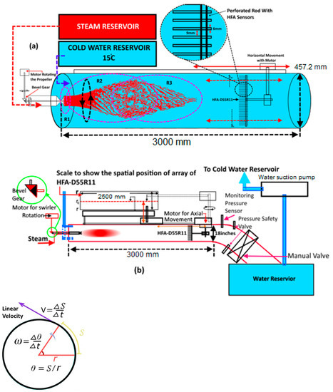
Figure 1.
A schematic of the experimental setup: (a) flow rig; (b) complete system along with linear and tangential velocities.
The value of the local density was estimated from temperature measurements of the fluid present at the specified time and spatial location with the help of the LM35 temperature sensors attached to each HFA sensor during calibration. For comparison, the average velocity was estimated using the relation as given below [20], using the fluctuations in data from each of the HFA sensors:
where is the water average velocity, is the probability density function, and is the signal amplitude. Relative errors existed in the measurements obtained by the sensors, which were in the range of 3–3.2%, corresponding to the velocity fluctuations against the inlet pressures of the steam and water (1–2 bars) at the 5 kHz sampling rate of the sensors, whereas the measurements were repeated 5 times (sampling duration, 5 min) in each phase of the experimentation to confirm the value of the relative error. The value of the corresponding error was subtracted from each measurement by each sensor before drawing the results.
The LM35 sensor’s relative errors range is from −0.750 °C to +0.750 °C, as mentioned in the manual for these sensors [17]. The wall-to-wall spacing between each pair of sensors is 9 mm, thereby leaving minor gaps on the top and bottom sides, where the velocity measurement facility through these sensors is not addressed, as the fluid flow profiles are inhibited by these regions, which is of no importance to our present goals. The data were acquired at a sample rate of 5 kHz and the total measurement time for each experimental phase was 5 min, with each phase being repeated 5 times to acquire the data with the most repetitions. The rod was traversed from the point ~50 cm apart from the nozzle exit at a rate of 0.5 cm towards the nozzle exit. The spatial resolution was changed to 0.1 cm in the second round of experiments, where the varying hydrodynamic nature of these flows was measured. Based on the nature of the velocity fluctuations and their derived amplitudes, the whole volume of the fluid domain was considered an ellipsoidal region, which was sub-divided into three small ellipsoidal regions, i.e., R1, R2, and R3 (Figure 1a). Region R1, comprising the two-dimensional space (based on the measurement strategy via vertical mounted HFA sensors), has a major axis length of ~10 cm. The half-length of this region is ~5 cm, which is between the point at the geometric center of the nozzle exit and 5 cm away from it. R2 comprises the ellipsoidal region, which has a major axis length of ~20 cm (i.e., extending from the nozzle exit to ~5 cm beyond the most swollen part of the swirling ellipsoidal volume). Region R3 has a major axis length of ~25 cm (which extends from the point ~5 cm before the most swollen part of the swirling body of the steam–water mixture to the point located just beyond the end of the swirling body of the steam–water mixture). There are overlapping regions that may arise due to this segregation of the whole region, which arises just to ensure that no space in the whole region should be left without characterization through the HFA sensor array. In the results, measurements of overlapping regions were not considered. As mentioned before, the motor was regulated and the transformer was used to rotate the propeller, which was calibrated for the frictional and inertial losses using the tachometer [15]. It was observed that inside the water at 15 °C, the errors in the rpm values measured by the tachometer ranged from 0.05 to 0.06% (3–18 rpm) at varying rotational speeds of 60–300 rpm, which were corrected by applying additional rpm from the motor in corresponding experimental phases to rotate the mixture of the steam and water at the mentioned rpm (Table 1).

Table 1.
Operating conditions.
The endpoint for this swirling body of the mixture of steam and water was inside the fluid region based on the amplitudes of the velocity fluctuations, which were measured prior to the injection of steam. The maximum normalized amplitude of the velocity fluctuations with the injection of cold water at 15 °C, as well as the rotation of the propeller at 300 rpm, corresponded to around ~0.5 cm. This amplitude was subtracted from each measurement to represent a true picture of the normalized amplitudes of the velocity fluctuations due to the swirling steam’s injection into the water only. The axial movement of the rod was controlled by another motor that had an axial shaft along which the rod was mounted with an array of HFA sensors. The sensors traversed the distance inside the flow rig. The operating conditions along with their respective ranges are presented in Table 1.
Since the whole of the flow rig was shut from the outside, to prevent pressure buildup inside the rig, a pressure safety valve, a pressure sensor, as well as a manually operated flow valve were provided at the start of the bent section. The amount of water added into the flow rig through the cold water injection at 15 °C as well as the condensation of the steam were equated with the help of the mentioned manual flow valve, through which the drained water was collected into a drain water reservoir, as shown in Figure 1b. The water was retained and injected at 15 °C into the flow rig from the cold water reservoir to prevent disturbances in the measurements of the HFA sensors due to the local boiling of the water at the sensor’s measurement face.
3. Results and Discussion
Both steam and water were injected at varying inlet gauge pressures of 1–2 bars, whereas the propeller was used to generate the swirling steam, which was rotated at rotational speeds of n = 60 and n = 300 rpm.
3.1. Ensembled Nature of the Normalized Amplitudes of the Velocity Fluctuations
In the current experimental setup, steam is injected in a swirling configuration into the water, which flows concurrently. The concurrently flowing water acts to impart shear force on the swirling steam body of the steam–water mixture, which leads to velocity fluctuations at the interface between the swirling steam and water flowing concurrently as a mixture, and this can be found from the attenuation of the normalized amplitudes of the velocity fluctuations. However, before looking into the results that were drawn from the observations, it is useful to briefly discuss the methodology that was used for the processing of the data. As outlined before, the data were acquired at a sampling rate of 5 kHz over 0.5 cm of the axial distance for 5 min across regions R1, R2, and R3. Therefore, a total of 15 million data points were recorded within R1, 45 million within region R2, and 60 million within region R3. The data were processed from each sensor based on the respective mean in each region (i.e., R1, R2, and R3) separately. The velocity fluctuations measured by each of the HFA sensors and their respective amplitudes were normalized by the respective mean amplitude of each HFA sensor in each region separately. The normalized amplitudes of these velocity fluctuations were found to decrease along the axial direction. This decrease was observed up to a certain point, corresponding to the vicinity of the most swollen portion of the steam–water swirling body along the axial axis, afterwards which point the trend changed and the velocity started increasing and then decreasing up to the end of the body of the swirling steam–water flow. This may have either been due to the contribution of the concurrently flowing water or due to the loss of strength (pressure drop along the axial direction) of the swirling steam–water volume inside the flow rig. Along the radial direction, these fluctuations increased, as measured by each of the HFA sensors with respect to their positions along the radial direction. This increase in the normalized velocity amplitudes shifted to large-scale fluctuations, which depicted that the sensors showing this trend were located across the steam–water swirling fluid’s interface with the concurrently flowing water. Thus, these measurements from the HFA sensors consolidate the idea that the velocity fluctuations and their respective normalized amplitudes exist inside a layer between the volumes of the two co-axial ellipsoidal areas, with one lying inside the other. The first (small) ellipsoidal volume is defined by the approximate proportionality or linearity of the variations in the velocity fluctuations along the radial direction inside the core ellipsoidal volume, while the second (larger) ellipsoidal volume is defined by the higher amplitude velocity fluctuations in the respective positions, thereby defining the layer in terms of the difference between their volumes. The thickness of this layer under the action of shear force by the concurrently flowing water decreases, which shows the attenuation of the normalized amplitudes under various operating conditions (as shown in Table 1). The attenuation of the velocity fluctuations is due to the decrease in thickness of the inhibiting layer across all regions in the absence and in the presence of the concurrently acting shear force at a maximum of 300 rpm, as can be seen in Figure 2a–c. Under the action of shear force, the thickness of the layer inhibiting flow instabilities cannot be decreased if the density of the fluid within the layer along the vertical axis is constant. In the present case, the density varies, so the thickness of the layer will also vary. These results are summarized further in terms of the variations in the volumes and surface areas of the respective ellipsoidal volumes, as shown by Figure 3. The first and fourth bar chart in Figure 3 support the conditions of no shear, whereas the rest of the bar charts depict the effects of the operating hydrodynamic conditions induced by shearing on the thickness of this layer, as well as the volume and surface areas.
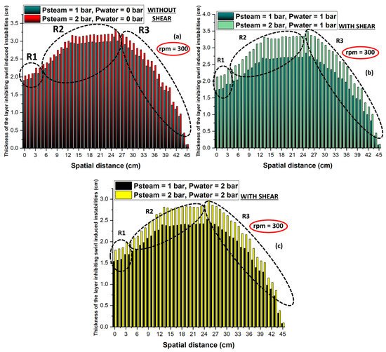
Figure 2.
(a) The thickness of the layer inhibiting the steam–water two-phase flow-induced velocity fluctuations. (a) The absence of concurrently acting shear forces and (b,c) the presence of concurrently acting shear forces under different steam and water pressures.
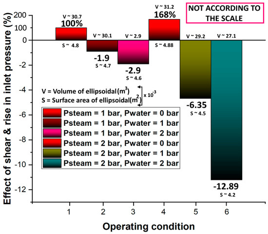
Figure 3.
Percentage reductions in the thickness of the layer inhibiting the steam–water two-phase flow-induced velocity fluctuations under the action of shearing from concurrently flowing water.
It has been observed that across some length scales, the shear force from the concurrently flowing water imparts a similar effect on these amplitudes, decreasing their values uniformly. Alternatively, the normalized amplitudes corresponding to the velocity fluctuations behave in an ensembled manner to the shear force, acting on the co-current swirling steam–water body across the length scale, where their originating velocity fluctuations are recorded. A possible reason for the observation of this behavior across some spatial positions, across which the uniform attenuation of the velocity fluctuations by the concurrently flowing water and shear force occurs, is presented as follows. A mixing layer between the two fluids that interact with each other in any orientation can be regarded as a Rayleigh layer [21,22,23], in which the velocity of the injected fluid itself sometimes becomes a source of filamentation of small scales at the outer surface of the injected fluid [24]. This concept helps us to understand the dynamics of the cascading turbulence. The inner core velocities are connected to the outer core mixing layer velocities linearly, wherein the mixing Rayleigh layer is composed of small unstable coherent structures with a fine filamentary nature [25]. Thus, if we consider the boundaries of the fluid layer exerting shear forces as static boundaries, the mixing Rayleigh layer interaction with the outer flowing fluid layers can be defined by the Rossby waves [26,27,28].
According to the picture portrayed by Bains and Mitsudra [29], the interaction of the mixing layers with the outer layers occurs in counter-propagation, which presents the possibility of enhanced constructive interaction and a phase-locking between these layers; on a contrary basis, any other flow orientation differing from the counter-propagation could inhibit the possibility of the non-constructive interaction, whereby the propagation due to the enhanced constructive interaction could be attenuated in an ensemble manner across a control plane. Thus, we can say that in such control planes under the length scale as defined previously, the rotational effects of the swirling fluids can perform a vital role to an extent, as contributed by the buoyancy and gravity waves, which impart a dominant influence on the evolution of the flow under certain shear forces [30]. The uniform attenuation effect imparted by the shear force from the concurrently flowing water has been shown in a similar manner before [24,30], as the shearing affects the stability of the flow in the vicinity of the rotating volume of fluids on a large scale; the filaments rapidly become aligned; and when constantly applying shear force, the instabilities are suppressed on a uniform basis.
The shear force acts to suppress the growth rate and reduce the range of unstable wave numbers. Such behavior sheds light on the cascading turbulence in terms of local interactions, thereby bringing down the shearing from the global scale to the small filament scale. The initial stretching of the length scale along the radial direction can lead into a control plan; however, when this scale is traversed to a certain length along the axial direction, ensembled normalized amplitudes of the velocity fluctuations occur. The effect of the non-dimensional swirl intensity (where is the horizontal distance from the nozzle outlet and is the diameter of the rig) against the initial swirl intensity (given by Equations (3) and (4)) [31] on the location of the control plane is shown in Figure 4:
where is the radius of the swirl and is the density of the fluid; in this case, we calculate the approximate density of the fluid at the respective spatial position with the help of the temperature of the fluid, i.e., either steam or water, using the LM35 temperature sensor [17]. Here, is the tangential velocity, which is determined using Equation (4), and is the axial velocity. It should be noted that the velocity fluctuations are measured across the flow rig, whereas Ux is the axial velocity, which is merely confined to the axial measurements. It should be noted that not only was the existence of the control plane confirmed by the repetition of the experiments. Changing the rpm of the propeller as well as replacing the base plate for the cold water injection with the new base plate, which had a different orientation of the water injection ports on the left-hand side of the rig, led to the value for the non-dimensionalized swirl intensity being equal to the value of the initial swirl intensity at the spatial location within the control plane. This point is referred to as the critical point where both swirl intensities are equal. The possible reasons for this critical point where the values of the are approximately equal to the S0 are illustrated in the following paragraph.
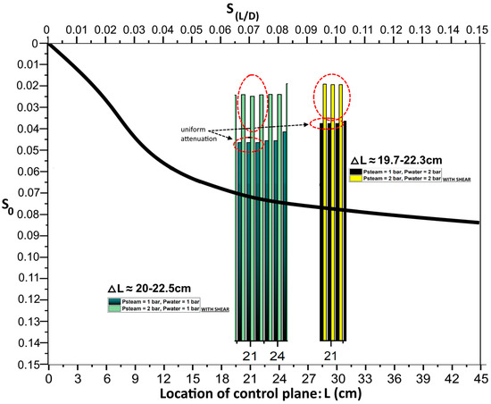
Figure 4.
Uniform attenuation of the swirl-induced flow instabilities by the shearing inside the control volume.
The Brunt–Väisälä frequency or buoyancy frequency is a measure of the stability of the fluid to the vertical displacements. In the present case, the swirl intensity S0 is measured at the position in the proximity of the steam nozzle and is measured along the axial axis, so this can be attributed to the frequency of the steam bubble’s inception and collapse inside the water domain. If this frequency is weak as compared to the rotational frequency, this will permit large amplitudes of the flow fluctuations. On a contrary basis, when the frequency of the buoyancy is more rapid than the frequency of the rotation, the amplitudes of the disturbances are not so significant [32,33] and the fluid layers can become stratified. In the present case, across all three regions, R1, R2, and R3, the equality of these two frequencies may be due to the delay in the propagation of the velocity fluctuations until those spatial positions at which , S0 ≈ 0.07. This equality condition exists within the uniform attenuation control plane length scale, so the role being played by the equality of these two frequencies in the uniform attenuation cannot be ignored in view of equating the effects of stabilizing and non-stabilizing factors.
3.2. Hydrodynamics of the Swirling Steam–Water Two-Phase Flow
The existence of spatial positions across which the swirling steam–water two-phase flow-induced velocity-fluctuation-based normalized amplitudes behave in an ensembled way was observed at varying inlet gauge pressure levels of the steam and water, i.e., 1–2 bars, and at varying rpm values of 60–300. The normalized amplitudes of the velocity fluctuations were investigated under three conditions, i.e., under the effect of shearing, which was investigated by varying the inlet pressures of the steam and concurrently flowing water; swirling, which was investigated by varying the rpm rates of the swirler; and discrete large-scale changes in the operating conditions. The details of these applied conditions and their outcomes are presented and discussed in the following paragraphs.
3.2.1. Hydrodynamic Nature of the Normalized Velocity Amplitudes under Shearing
The normalized velocity amplitudes were estimated based on the velocity fluctuations across the three regions, namely R1, R2, and R3. As mentioned before, during the analysis of the normalized amplitudes of velocity fluctuations, the amplitudes were measured against the normalized velocity fluctuations under the shear force acting on the swirling steam–water flow in an ensemble way.
It was observed that along a radial line segment, we could define a length using certain spatial points by traversing the HFA sensor array along the axial direction away from the exit of the nozzle. Under varying conditions of the inlet pressure and a fixed rotational speed, i.e., 300 rpm (higher swirl intensity S0 at the exit of the nozzle), it was observed that the normalized amplitudes of the velocity fluctuations at these spatial positions showed varying behaviors under the effects of the shear force acting on this region from the concurrently flowing water.
First, it should be noted that the spatial resolution for the observation of this behavior was 0.1 cm, i.e., the vertically mounted HFA sensors were traversed at a discrete spatial step of 0.1 cm. Thus, the measurements being collected over the increased spatial resolution of the fluid region totaled about 600 million data points across all regions, i.e., R1, R2, and R3, at the maximum rotation speed of 300 rpm. Further, it was observed in the first case that after the onset of a steam and water injection at 1 bar of gauge pressure, the velocity fluctuations showed an ensembled nature over an area with a length of ~2.1 cm, with ~6.3% of the total data points showing ensembled normalized behavior in view of the normalized amplitudes of the velocity fluctuations. When the shear was increased in the second case, corresponding to 2 bars of the gauge pressure for the water, the values of the normalized amplitudes of the velocity fluctuations were reduced and the area at which these normalized velocity fluctuation amplitudes prevailed was stretched, with a total increase of ~1.2% as compared to the total area where these amplitudes prevailed at 1 bar of gauge pressure.
Thus, it was observed that in the first two cases, i.e., Ps and Pw = 1 bar and Ps and Pw = 2 bars, the spatial distance across which the ensemble normalized amplitudes of the velocity fluctuations were found increased by ~1.2%. In the third and fourth cases, i.e., Ps = 2 bars and Pw = 1 bar and Ps = 2 bars and Pw = 2 bars, the number of these ensembled normalized amplitudes of the velocity fluctuations increased, with a total of 4.7% of the fluctuations showing an ensembled nature. These ensembled amplitudes of the velocity fluctuations in case 4 prevailed at a length that was 2.7% longer than the length at which the amplitudes prevailed in case 3.
Thus, we can safely say that under the action of the shear-induced stretching exerted by the concurrently flowing water, as well as by keeping in mind the unstable fluctuating nature of the steam inside the water and the relative error in the HFA measurements (3–3.2%), the swirling steam–water two-phase flows showed a nearly proportional varying nature in view of the ensembled normalized velocity amplitudes across the spatial length scale.
3.2.2. Normalized Velocity Amplitudes under the Action of Shearing
The hydrodynamic characteristics of the swirling steam–water two-phase flows were investigated under the action of the operating conditions. It was observed that the effect of the stretching was imparted on the ensembled normalized amplitudes of the velocity fluctuations in view of an increase in the number of their occurrences as well as stretching in an area on a proportional basis. Here, the effect of the swirl intensity was investigated on the swirling steam–water two-phase flows. The propeller’s non-dimensionalized swirl intensity rates S0 at the exit of the steam nozzle varied from 0 to 0.15, with the maximum values used for the rest of the hydrodynamic conditions, i.e., Ps and Pw = 2 bars. Further, it was found that by segregating the values of the swirling intensity into three blocks, i.e., (0–0.05), (0.05–0.10), and (0.10–0.15), the effect of the increase in non-dimensionalized swirling intensity on the area under the influence of the ensembled normalized amplitudes of the velocity fluctuations was imparted on a proportional basis. Initially, with an increase in the values of the non-dimensionalized swirling intensity S0 from 0 to 0.05, the thickness of the layer, i.e., the radial distance across which the amplitudes travelled increased to around 0.7%. The length scale under the influence of the ensembled normalized amplitudes of the velocity fluctuations was increased to a length of 1.81 cm, with the total number of ensembled normalized amplitudes of the velocity fluctuations being approximately equal to 0.18% of the total number of velocity fluctuation amplitudes across this length. Further, with an increase in the values of the non-dimensionalized swirling intensity from 0.05 to 0.10, the thickness of the layer was increased by around 0.82% and the length under the influence of the ensembled normalized amplitudes of the velocity fluctuations was increased to 1.7%. With a further increase in the values of the non-dimensionalized swirling intensity S0 from 0.10 to 0.15, the thickness of the layer was increased to around 1%, with the length under the influence of these ensembled normalized amplitudes of the velocity fluctuations increasing to 2.1%. Thus, we can safely say that under the action of the swirling exerted by the propeller, while also keeping in mind the unstable fluctuating nature of the steam inside the water and the relative errors in the HFA measurements (3–3.2%), the swirling steam–water two-phase flows showed a nearly proportional nature under the action of swirling in terms of the ensembled normalized velocity amplitudes across the length scale.
3.2.3. Normalized Velocity Amplitudes under Large Discrete Variations in Inlet Hydrodynamic Conditions
The steam–water two-phase flows were investigated under the action of stretching as well as swirling. It was observed that the two-phase fluid flow exhibited a nearly proportional nature in terms of the number of ensemble average velocity fluctuation magnitudes under the action of the mentioned conditions. Here, in order to confirm the nature of these flows under discrete large-scale variations of the hydrodynamic conditions, we used two sets of operating conditions. In the first set, both the steam and water were injected at the same 1 bar of gauge pressure at 60 rpm. In the second set of operating conditions, both the steam and water were injected at the same pressure of 2 bars of gauge pressure at S0 = 0.15. For this purpose, the steam and water concurrent injection was controlled by a solenoid valve, which was controlled electronically with a delay time of 0.001 s. The speed of the motor was controlled by another DC motor, which was regulated for a step increase of n = 300 rpm, with a delay time of 0.01 s. The difference in these delays could play a significant role if the length scale for the ensemble velocity fluctuates within the vicinity of the steam nozzle exit. However, these delays were ignored, as the propagation of these effects by the steam and water imparted respective variations in the inlet injection pressures, as well as variations in rpm, while S0 was measured approximately at a distance greater than ~20 cm away from the nozzle exit (Figure 4). It was observed that in the first case, i.e., at Ps and Pw = 1 bar at rpm = 60, the length scale was equal to a length of ~1.91 cm, with 0.9% of the total length along the radial direction showing these ensembled amplitudes of the velocity fluctuations.
In the second case, i.e., at Ps and Pw = 2 bar at n = 300 rpm, the length scale increased to around ~4.9%, where the ensembled normalized amplitudes of the velocity fluctuations were observed. Thus, if we consider the number of these ensembled normalized amplitudes of the velocity fluctuations/cm as the response of the steam–water two-phase flow system to the discrete variation of the hydrodynamic conditions, along with the variations in the length scale across which these ensembled normalized amplitudes of the velocity fluctuations were recorded, we can say that the steam–water two-phase flow system responded to the discrete large-scale variations of the hydrodynamic operating conditions on a proportionally varying basis. Thus, we can safely say that by keeping in mind the unstable fluctuating nature of the steam inside the water and the relative errors in the HFA measurements (3–3.2%), the swirling steam–water two-phase flows showed a nearly varying proportional nature in terms of the ensembled normalized velocity amplitudes across the length scale under the action of discrete large-scale changes in the hydrodynamical conditions.
4. Conclusions
In the current manuscript, the steam–water swirling flow domain was investigated under the actions of three varying operating hydrodynamic conditions. The steam and water were both injected at gauge pressures of 1.0 and 2.0 bars, whereas the swirling steam was injected using a propeller, which rotated at rotational speeds of 60 and 300 rpm. It was observed that the velocity fluctuations with the ensemble amplitudes were inhibited inside a layer that can be defined based on the spatial locations of the points where these ensemble amplitudes of the velocity fluctuations were observed. The ensemble amplitudes of the velocity fluctuations showed a proportional nature under the action of the stretching, which acted on the shearing of the concurrently flowing water at varying inlet pressures; the swirling, which acted by varying the non-dimensionalized rotating propeller swirling intensity levels; and a discrete large-scale variation in the hydrodynamic operating conditions. Across the control plane defined by the thickness and length at which these normalized amplitudes of the velocity fluctuations were observed, under the action of shearing, swirling, and a discrete large-scale variation in the operating hydrodynamic conditions, the swirling steam–water two-phase flows almost showed proportional varying nature.
Author Contributions
Conceptualization, H.A.S.G., and A.K.; methodology, K.S.; validation, A.K., K.S.; formal analysis, A.K. and H.A.S.G.; investigation, K.S. and H.A.S.G.; resources, K.S. and H.A.S.G.; data curation, A.K.; writing—original draft preparation, A.K. and K.S.; writing—review and editing, K.S.; visualization, A.K. and K.S.; supervision, K.S. and H.A.S.G.; project administration, H.A.S.G.; funding acquisition, H.A.S.G., K.S., and A.K. All authors have read and agreed to the published version of the manuscript.
Funding
The project was funded by the Deanship of Scientific Research (DSR) at Jazan University, Jazan, Kingdom of Saudi Arabia, under grant no. W43-063.
Data Availability Statement
The data will be available upon request.
Acknowledgments
The authors are thankful to the Deanship of Scientific Research (DSR) at Jazan University, Jazan, Kingdom of Saudi Arabia, for supporting this work through grant no. W43-063m and Dongguan University of Technology (DGUT), Sino-French United Institute (DCI), for their support and cooperation.
Conflicts of Interest
The authors declare no conflict of interest.
References
- Huang, Y.; Yang, V. Effect of swirl on combustion dynamics in a lean-premixed swirl-stabilized combustor. Proc. Combust. Inst. 2005, 30, 1775–1782. [Google Scholar] [CrossRef]
- Waugh, D.W.; Plumb, R.A.; Atkinson, R.J.; Schoeberl, M.R.; Lait, L.R.; Newman, P.A.; Loewenstein, M.; Toohey, D.W.; Avallone, L.M.; Webster, C.R.; et al. Transport out of the lower stratospheric Arctic vortex by Rossby wave breaking. J. Geophys. Res. 1994, 99, 1071–1088. [Google Scholar] [CrossRef]
- Khan, A.; Haq, N.U.; Chughtai, I.R.; Shah, A.; Sanaullah, K. Experimental investigations of the interface between steam and water two phase flows. Int. J. Heat Mass Transf. 2014, 73, 521–532. [Google Scholar] [CrossRef]
- Khan, A.; Takriff, M.S.; Rosli, M.I.; Othman, N.T.A.; Sanaullah, K.; Rigit, A.R.H.; Shah, A.; Ullah, A.; Mushtaq, M.U. Turbulence dissipation and its induced entrainment in subsonic swirling steam injected in cocurrent flowing water. Int. J. Heat Mass Transf. 2019, 145, 118716. [Google Scholar] [CrossRef]
- Tennekes, H.; Lumley, J.L. A First Course in Turbulence; MIT Press: Cambridge, MA, USA, 1972. [Google Scholar]
- Townsend, A.A.R. The Structure of Turbulent Shear Flow; Cambridge University Press: Cambridge, UK, 1976. [Google Scholar]
- Moore, D.W.; Saffman, P.G. Structure of a Line Vortex in an Imposed Strain. In Aircraft Wake Turbulence; Springer: Boston, MA, USA, 1971; pp. 339–354. [Google Scholar] [CrossRef]
- Kida, S. Motion of an elliptic vortex in a uniform shear flow. J. Phys. Soc. Jpn. 1981, 50, 3517–3520. [Google Scholar] [CrossRef]
- Legras, B.; Dritschel, D. Vortex stripping and the generation of high vorticity gradients in two-dimensional flows. Appl. Sci. Res. 1993, 51, 445–455. [Google Scholar] [CrossRef]
- Gupta, A.K.; Lilley, D.G. Combustion and environmental challenges for gas turbines in the 1990s. J. Propuls. Power 1994, 10, 137–147. [Google Scholar] [CrossRef]
- Shtern, V.; Hussain, F. Collapse, symmetry breaking, and hysteresis in swirling flows. Annu. Rev. Fluid Mech. 1999, 31, 537–566. [Google Scholar] [CrossRef]
- Paschereit, C.O.; Gutmark, E.; Weisenstein, W. Excitation of Thermoacoustic Instabilities by Interaction of Acoustics and Unstable Swirling Flow. AIAA J. 2000, 38, 1025–1034. [Google Scholar] [CrossRef]
- Tangirala, V.; Chen, R.H.; Driscoli, J.F. Effect of Heat Release and Swirl on the Recirculation within Swirl-Stabilized Flames. Combust. Sci. Technol. 1987, 51, 75–95. [Google Scholar] [CrossRef]
- Ogawa, A. Vortex Flow; CRC Press: Boca Raton, FL, USA, 1993. [Google Scholar]
- Omega Engineering, Digital Tachometer|Omega Engineering, (n.d.). Available online: https://www.omega.com/en-us/sensors-and-sensing-equipment/motion-vibration-and-speed/speed-sensors/p/OMDC-DM8000- (accessed on 30 June 2023).
- Probes for Hot-wire Anemometry, n.d. Available online: https://www.labima.unifi.it/upload/sub/Strumentazione/Manuali/DANTEC%20-%20Anemometry.pdf (accessed on 30 June 2023).
- LM35 LM35 Precision Centigrade Temperature Sensors. 1999. Available online: www.ti.com (accessed on 3 August 2019).
- Katarzhis, A.K. Electrical Method of Recording the Stratification of a Steam-Water Mixture. 1958. Available online: https://apps.dtic.mil/docs/citations/AD0153417 (accessed on 30 June 2023).
- Hsu, Y.Y.; Simon, F.F.; Graham, R.W. Application of hot-wire anemometry for two-phase flow measurements such as void fraction and slip velocity. In Proceedings of the ASME Winter Annual Meeting, Philadelphia, PA, USA, 17–22 November 1963. [Google Scholar]
- Delhaye, J.M.; Galaup, J.P. Hot-Film Anemometry in Air-Water Flow. In Scholars’ Mine Symposia on Turbulence in Liquids Chemical and Biochemical Engineering; Missouri University of Science and Technology: Rolla, MO, USA, 1975; Available online: https://scholarsmine.mst.edu/sotilhttps://scholarsmine.mst.edu/sotil/11 (accessed on 8 October 2019).
- Drazin, P.G. Introduction to Hydrodynamic Stability; Cambridge University Press: Cambridge, UK, 2002. [Google Scholar]
- Rayleigh, J.W.S.B. The Theory of Sound; McMillan: Ottawa, ON, Canada, 1888. [Google Scholar]
- Regev, O.; Umurhan, O.M.; Yecko, P.A. Modern Fluid Dynamics for Physics and Astrophysics; Springer: Berlin/Heidelberg, Germany, 2016; p. 680. [Google Scholar]
- Dritschel, D.G. On the stabilization of a two-dimensional vortex strip by adverse shear. J. Fluid Mech. 1989, 206, 193–221. [Google Scholar] [CrossRef]
- Bretherton, F.P. Baroclinic instability and the short wavelength cut-off in terms of potential vorticity. Q. J. R. Meteorol. Soc. 1966, 92, 335–345. [Google Scholar] [CrossRef]
- Hoskins, B.J.; Mcintyre, M.E.; Robertson, A.W. On the use and significance of isentropic potential vorticity maps. Quart. J. R. Met. Soc. 1985, 111, 877–946. Available online: http://speedy.aos.wisc.edu/Hoskins_etal_1985.pdf (accessed on 30 June 2023). [CrossRef]
- Carpenter, J.; Tedford, E.; Heifetz, E.; Lawrence, G. Instability in Stratified Shear Flow: Review of a Physical Interpretation Based on Interacting Waves. Appl. Mech. Rev. 2011, 64, 060801. [Google Scholar] [CrossRef]
- Heifetz, E.; Bishop, C.H.; Alpert, P. Counter-propagating Rossby waves in the barotropic Rayleigh model of shear instability. Q. J. R. Meteorol. Soc. 2007, 125, 2835–2853. [Google Scholar] [CrossRef]
- Biancofiore, L.; Gallaire, F.; Heifetz, E. Interaction between counterpropagating Rossby waves and capillary waves in planar shear flows. Phys. Fluids 2015, 27, 044104. [Google Scholar] [CrossRef]
- Dritschel, D.D.G. The Stability of Filamentary Vorticity in Two-Dimensional Geophysical Vortex-Dynamics Models. 1991. Available online: http://www-vortex.mcs.st-and.ac.uk/~dgd/papers/wd91.pdf (accessed on 30 June 2023).
- Vaidya, H.A.; Ertunç, Ö.; Genç, B.; Beyer, F.; Köksoy, C.A. Delgado, Numerical simulations of swirling pipe flows- decay of swirl and occurrence of vortex structures. J. Phys. Conf. Ser. 2011, 318, 062022. [Google Scholar] [CrossRef]
- Vallis, G.K. Atmospheric and Oceanic Fluid Dynamics; Cambridge University Press: Cambridge, UK, 2017. [Google Scholar] [CrossRef]
- Walker, J.M. Atmospheric convection. Int. J. Climatol. 1995, 15, 821–822. [Google Scholar] [CrossRef]


Disclaimer/Publisher’s Note: The statements, opinions and data contained in all publications are solely those of the individual author(s) and contributor(s) and not of MDPI and/or the editor(s). MDPI and/or the editor(s) disclaim responsibility for any injury to people or property resulting from any ideas, methods, instructions or products referred to in the content. |
© 2023 by the authors. Licensee MDPI, Basel, Switzerland. This article is an open access article distributed under the terms and conditions of the Creative Commons Attribution (CC BY) license (https://creativecommons.org/licenses/by/4.0/).