Article

Numerical Modelling of Water Flashing at Sub-Atmopsheric Pressure with a Multi-Regime Approach

by
Clément Loiseau
1,2,*,
Stéphane Mimouni
1,2,
Didier Colmont
1 and
Stéphane Vincent
2
1
R&D Division, Electricité de France (EDF), 78400 Chatou, France
2
Laboratoire Modélisation et Simulation Multi-Echelle (MSME), CNRS, Université Gustave Eiffel, Université Paris-Est Créteil, 77420 Marne-la-Vallée, France
*
Author to whom correspondence should be addressed.
Fluids 2023, 8(5), 143; https://doi.org/10.3390/fluids8050143
Submission received: 22 March 2023 / Revised: 18 April 2023 / Accepted: 24 April 2023 / Published: 28 April 2023
(This article belongs to the Special Issue Advances in Numerical Methods for Multiphase Flows, Volume II)

Abstract

:
The CFD numerical study of the flash boiling phenomenon of a water film was conducted using an Euler–Euler method, and compared to the experiments on the flashing of a water film. The water film is initially heated at temperatures ranging from 34 to 74 C (frim 1 to 41 C superheat), and the pressure is decreased from 1 bar to 50 mbar during the experiments. This paper shows that the experiments could not be correctly modelled by a simple liquid/bubble model because of the overestimation of the drag force above the water film (in the gas/droplet region). The generalised large interface model (GLIM), however, a multi-regime approach implemented in the version 7.0 of the neptune_cfd software, is able to differentiate the water film, where liquid/bubble interactions are predominant from the gas region where gas/droplet interactions are predominant, and gives nice qualitative results. Finally, this paper shows that the interfacial heat transfer model of Berne for superheated liquids could accurately predict the evolution of the water temperature over time.

1. Introduction

Flashing, flash evaporation, or flash boiling, is a rapid pressure decrease which causes the liquid to reach a metastable state with P l ( T l ) < P s a t ( T l ) . The excess of energy is transformed into latent heat through the production of bubbles until the liquid returns to a stable state [1].
Flashing differs from wall boiling because the bubbles develop inside the liquid (bulk nucleation), or at the interface between the liquid and the gas, and not exclusively at the wall. It differs from evaporation because mass transfer can take place inside the liquid with the creation of bubbles, and not only at the interface between the liquid phase and the gas phase.
The flash boiling of water at sub-atmospheric pressure is involved in the vacuum drying process where the decrease in the pressure leads to the vaporisation of the liquid water and to the vacuuming of the vapour. This process is used in several industries, such as the salt industry with water desalination [2], the paper industry with paper drying [3], and the nuclear industry with the drying of failed fuel rods. Flash boiling has been studied experimentally at sub-atmospheric pressures, and both experimentally and numerically at a very high pressure with the Super Moby Dick [4,5] and the SUPERCANON [6] experiments. However, numerical simulations of the flashing phenomenon at sub-atmospheric pressures are rare.
Fluids 08 00143 i001

1.1. Experiments at Sub-Atmospheric Pressure

The experiments conducted on the flashing of a water film at sub-atmospheric pressure by Miyatake et al. [7], Gopalakshrishna et al. [8] and Saury [1] are relatively similar. A flash chamber with a small volume is initially partially filled with heated water. A vacuum chamber with a much larger volume (almost 300 times larger in the experiment of Saury) is then depressurised until the experimental pressure is reached. At the start of the experiment, a valve is opened to connect both chambers. This leads to the quick depressurising of the flash chamber, and to the flashing of the liquid film. The quantity of interest in these experiments is the evolution of the evaporated mass of water over time. However, this quantity cannot be measured easily, which is the reason why the authors decided to extrapolate it from the evolution of temperature over time.
The experimental facility used by Saury is more thoroughly described in Section 3.

1.2. Bibliographical Synthesis of the Flash Boiling Models

The first approach to modelling the flashing phenomenon was proposed by Miyatake et al. [7]. The authors defined a dimensionless number, the non-equilibrium function (NEF), to represent the evolution of the evaporated mass.
N E F ( t ) = m e v ( ) m e v ( t ) m e v ( )
m e v ( ) represents the evaporated mass at the end of the experiment in the steady state. m e v ( t ) represents the evaporated mass of water at a time t. Assuming that all the heat is used to vaporise the liquid ( m c p d T d m h f g = 0 ), and that the physical properties of the liquid are constant, they found m e v = m 0 ( 1 exp ( c p h f g ( T 0 T ) ) , with m 0 being the initial mass of liquid. c p / h f g is small, typically O ( 10 3 ) K 1 ; therefore, the Taylor expansion of the exponential (Equation (2)) gives a good approximation of m e v .
m e v = m 0 c p h f g ( T 0 T )
Finally it was possible to rewrite the NEF as a function of the temperature.
N E F ( t ) = T ( t ) T e T 0 T e
T e is defined as the final temperature of the liquid, that is to say the saturation temperature at the final pressure. T 0 is the initial temperature. Using the experimental evolution of the NEF over time, he showed that flash boiling can be separated into two stages. In the first stage, the temperature and thus the NEF quickly decrease because of the boiling. During the second stage, the decrease is slower because boiling only takes place at the interface. The flashing time is defined at the intersection between these two stages. No explanation was given by the authors about the physical phenomenon which leads to boiling at the interface in the second stage. An explanation for that will be proposed in Section 4.3.
Miyatake et al. proposed a correlation giving the NEF as a function of the time t, the equilibrium temperature T e (the saturation temperature at the final pressure), and the superheat Δ T .
N E F ( t ) = ( 1 + 2.8 × 10 3 T e 1.3 Δ T ) t 44 T e 0.86 Δ T 0.55
Later, Gopalakrishna et al. [8] published another correlation which gives the evaporated mass over time based on the Jakob number, the Prandtl number, and on the pressure superheat Δ P = P s a t P . In 2003, Saury [1] published several dimensionless correlations on the maximum evaporation rate, the flashing time, and the evaporated mass as a function of the initial temperature T 0 , the depressurising rate d P d t , the superheat Δ T , and the water film height h.
Using these correlations, it is possible to predict the evaporated mass of water over time in separated effect experiments where the final temperature T e and the liquid superheat Δ T are known. However, these correlations require the knowledge of the pressure evolution over time. Furthermore, they do not give information on local phenomena. Therefore, to predict the evaporated mass in a more realistic situation, numerical models are necessary.
Augusti et al. [9] suggested a mathematical model to simulate the flashing phenomenon. The ideal gas law is used to write the evaporated mass of water as a function of the vapour pressure at the free surface P v , F S .
m e v = t [ ( P s a t P v , F S ) V V L M H 2 0 R T ]
Some correlations giving P v , F S as a function of the temperature, the liquid volume and the flashing time were then obtained from a series of experiments. These correlations were validated for the geometry of the experimental facility, initial volumes of water in the [0, 100] mL range, and initial temperatures between 20 and 40 C. V V L is defined as the volume of the “vaporisation layer”. The authors proposed a correlation for this vaporisation layer, involving the initial temperature T 0 , the initial volume V, and the time t.
Recently, Wang et al. [10] published a method to simulate the flash evaporation using a heat balance equation.
d m e v d t = ( ( λ g L c N u ( T g T l ) + q ) A f m l c p , l d T l d t ) / h f g
λ g is the thermal conductivity of the gas mixture, A f = π R 2 is the area of the water film where R is the radius of the flash chamber, L C = A f is a characteristic length, q is the heat flux (the flash chamber was heated in this experiment), and h f g is the latent heat. In order to compute d T l / d t , the thermal follow-up coefficient (TFC) was defined. This coefficient determines the evaporated mass of water without having to know the equilibrium temperature (unlike the NEF defined by Miyatake).
T F C ( p 1 , p 2 ) = T l p 2 T l p 1 T s a t p 2 T l p 1
p 1 and p 2 are the pressure of the liquid at times t 1 and t 2 , respectively. TFC describes the ratio between the actual temperature drop and the ideal temperature drop. Equations (8) and (9) show how temperature at time t p i + 1 is computed using the TFC.
d T l d t = T F C i + 1 T s a t p i + 1 T l p i d t
T l p i + 1 = T l p i + T F C i + 1 ( T s a t p i + 1 T l p i )
Wang et al. established a correlation between the TFC and the depressurisation rate dp/dt. They observed that the TFC was always below the line 4.5 × 10 4 ( d p d t ) + 0.01 . Consequently, they decided to multiply this line by the random function R n d ( 0 , 1 ) between 0 and 1.
T F C = ( 4.5 × 10 4 ( d p d t ) + 0.01 ) × R n d ( 0 , 1 )
The models and correlations developed by Augusto and Wang et al. gave good results on their experiments. However, unlike numerical models, these programs cannot be directly used on other flashing experiments because their correlations can be out of the validation range. Additionally, local phenomena, such as the bubble density, can only be modelled using numerical models. Therefore, some authors, such as Enoki et al. [11], modelled flow boiling in mini-channels using a regime-based approach. In these approaches, the flow regime (bubbly, slug, churn, annular, droplet) is determined using dimensionless empirical correlations. The head losses and heat transfer coefficients are then computed using correlations, such as the Lockhart–Martinelli model for head losses. However, the correlations used in these models might not give good results outside of their validation range. Furthermore, the slug, churn and annular regimes are well defined in mini-channels, but it is unclear how these models can be applied to pool flashing.
That is why it was decided to model the experiments of Saury using CFD, with the neptune_cfd software to improve the knowledge of the flashing of a liquid film.
Section 2 presents the numerical models used in the simulations. Section 3 describes the experimental facility used by Saury to study the flashing of the liquid film. Finally, Section 4 compares the experimental and numerical results.

2. Models

2.1. The Neptune_cfd Code

To simulate the experiments of Saury, the neptune_cfd software was used. It was developed by Electricité de France (EDF), Commissariat à l’Energie Atomique et aux Energies Alternatives (CEA), Institut de Radioprotection et de Sûreté Nucléaire (IRSN), and Framatome. It is a computational fluid dynamic code based on the two-fluid model of Ishii [12] and Delhaye et al. [13] for the modelling of two-phase flow in 3D. Density, viscosity, volume fraction and local velocity are defined for each field in each cell. The solver is implemented in the neptune_cfd environment [14,15]. It is based on a finite volume discretisation together with a collocated arrangement for all variables. A common pressure is assumed for all fields. A semi-implicit method for the pressure-linked equations (SIMPLE) solver is used in the code neptune_cfd. An iterative coupling of these equations is applied to ensure mass conservation (and energy conservation for non-isothermal flows).

2.2. Equations Solved

In this study, two fields are considered: the liquid water, noted with the subscript l, and the gas, a mixture of air and vapour, noted with the subscript g. For each field k, three balance equations are solved: mass conservation, momentum balance and energy conservation.
t ( α k ρ k ) + x i ( α k ρ k u k , i ) = Γ k
t ( α k ρ k u k , i ) + x j ( α k ρ k u k , i u k , j ) = x j ( α k τ k , i j + Σ k , i j R e ) α k P x i + α k ρ k g i + I k
t ( α k ρ k H k ) + x j ( α k ρ k H k u k , j ) = x j ( α k u k , i τ k , i j ) x j ( α k Q k , j ) + α k P t + α k ρ k u k , i g i + Π k + I k , i u k , i
Γ k is the interfacial mass transfer, τ k the viscous stress tensor, Σ k , i j R e , the turbulent stress tensor, I k is the interfacial momentum transfer, Q k = λ k T k is the conductive heat flux, and Π k is the interfacial enthalpy transfer.
An R i j ϵ model [16] is used on both the liquid and the gas to model the turbulence ( Σ k , i j R e ). The physical properties ( c p , k , ρ k , μ k , λ k etc) are computed using the CATHARE tables. α k , u k , H k , and P are solved using the balance equations and the equation α l + α g = 1 .
The interfacial terms ( Γ k , I k , and H k ) are solved with interfacial closure laws.
It should be noted that the interfacial enthalpy transfer Π k can be split into two terms:
Π k = Γ k h k + Π k
Γ k h k is the latent heat transfer, caused by mass transfer. Π k is the sensible heat transfer, which does not depend on the mass transfer. The mass and energy conservation give:
Γ l + Γ g = 0
Π l + Π g = 0
Using Equations (14)–(16), it is possible to express Γ k as a function of Π k .
Γ l = Γ g = Π l + Π g h g h l
Hence, only I l , I g , Π l , and Π g need to be modelled to close the system. The expression of these interfacial terms depends on the model used.
Finally, a transport equation is solved for the air to determine the air mass fraction y a i r (and as a result, y v a p = 1 y a i r ).
t ( α g ρ g y a i r ) + x j ( α g ρ g u g , j y a i r ) = x j ( α g ρ g u a i r d i f f y a i r )
u a i r d i f f is given by Fick’s law.

2.3. The Liquid/Bubble Model

The first approach used in this paper is the dispersed liquid/bubble model. This model was validated on many experiments involving bubbly flows from the neptune_cfd validation basis, and in particular, on bulk-boiling experiments [4]. In this approach, the liquid is considered continuous, while the gas is a dispersed field in the form of subgrid bubbles, characterised by their diameter d b and area concentration A i . A transport equation is solved to compute the bubble interfacial area concentration A i . As the bubble diameter was not measured experimentally, an arbitrary value of the bubble diameter was taken in this study ( d b = 1 mm). The subgrid coalescence/fragmentation of the bubbles was not considered, which seems reasonable given the experimental conditions (the initial liquid height is h = 15 mm).

2.3.1. Interfacial Momentum Transfer

Five interfacial forces I k are considered in the bubble model: the drag force of Ishii [17], the lift force of Tomiyama [18], the Zuber-added mass force [19], a turbulent dispersion force and a wall force. In this section, only the expression of the drag force (the most important force by far in the experiment) is presented.
Equation (19) gives the momentum transfer from the liquid to the bubbles F b D resulting from the viscous drag force.
I b D = 1 8 A i ρ l C D | | u b u l | | ( u l u b )
A i = 6 α b / d b is the volumic interfacial area, and C D is the drag coefficient expressed using the empirical model of Ishii [17].

2.3.2. Interfacial Enthalpy Transfer

As for the interfacial enthalpy transfer, a “time-step return to saturation” model is used for the gas. This model keeps the vapour at its saturation temperature.
Π g = α l α g ρ g c p , g τ r e l a x ( T s a t T g )
τ r e l a x , the time to saturation term was picked equal to 10 2 s.
The model of Berne [20] is used to model the flashing of the liquid in a superheated state ( h l > h s a t ). It should be noted that the interfacial enthalpy transfer is modelled as a function of ( h s a t h l ) instead of ( T s a t T l ) to take the pressure variation into account. Furthermore, the Berne coefficient C b e r n e characterises the flashing speed.
Π l = C b e r n e A i ( h s a t h l )
A i = 6 α l d b is the interfacial area concentration. The value of α l used to compute the interfacial area is taken as the maximum between the actual volume fraction and 10 15 . This numerical choice makes bulk nucleation possible. C b e r n e is a coefficient given by Equation (22).
C b e r n e = m a x ( λ l c p , l d b N u 1 , λ l c p , l d b N u 2 , 12 π d b c p , l a b )
where N u 1 = 4 P e π , N u 2 = 2 , a = ρ l ρ g and b = λ l c p , l h f g . P e = R e l . P r l is the Péclet number.

2.4. The Generalised Large Interface Model (GLIM)

The second model used in this paper is the GLIM (presented in detail in [21,22,23]). The GLIM was developed to model multi-regime two-phase flows. In each cell, at each time step, it models large bubbles and stratified flows using a large interface approach when the cells are small enough. If the cells are too big to represent the bubbles/droplets, a subgrid bubble/droplet model is used. This idea is summarised in Figure 1, where the left and right pictures show a cell with subgrid bubbles and droplets, respectively. The middle picture shows a bubble with a diameter larger than the cell size Δ x . In this case, a large interface model is used.
It should be noted that, unlike regime-based models ([11,24], for example), the GLIM does not rely on empirical correlations to predict the flow regimes. In these approaches, the regime (bubbly, slug, churn, annular, droplet…) is predicted using empirical correlations involving dimensionless numbers. The heat transfer coefficient is then predicted from correlations validated in the flow regime.
The main challenge with the GLIM approach is to find the correct criteria to switch from the three different models shown in Figure 1. Experimental studies of bubbly flows [25,26,27] showed that the gas volume fraction α g can rarely be higher than 0.4 for bubbly flows. Applying the same to droplet flows, it is assumed that α g can rarely be smaller than 0.6 for droplet flows.
As for the transition between the dispersed models and the LIM, the criterion presented in Equation (23) is used. At the interface between a large bubble and a continuous liquid, the liquid fraction varies from 1 to 0 in three cells ( | | α l | | 0.33 Δ x ). To be guaranteed to catch the interface when the continuous liquid contains subgrid bubbles, the critical value of the gradient was set to 0.2 Δ x .
Large Interface model i f   | | α l | | 0.2 Δ x Dispersed model ( bubble or droplet ) e l s e
The three models used in the GLIM (the bubble model, the droplet model, and the large interface model) were validated separately on many experiments from the validation basis of neptune_cfd ([28,29] for the droplet model [30] for the LIM). The combination of these three models into the GLIM was validated on adiabatic cases, such as the emptying of a bottle [22] and on several cases involving heat and mass transfer (condensing two-phase flows in mini-channels [23]). The modelling of Saury’s experiments on flash boiling in this article aim to expand the validation range of the GLIM.
For large interfaces, the model of Coste [30] is used. In this case, the interfacial enthalpy transfer is computed using the Coste wall law model (24).
Π l = C C o s t e ( T s a t T l )
where C C o s t e is an empirical coefficient.
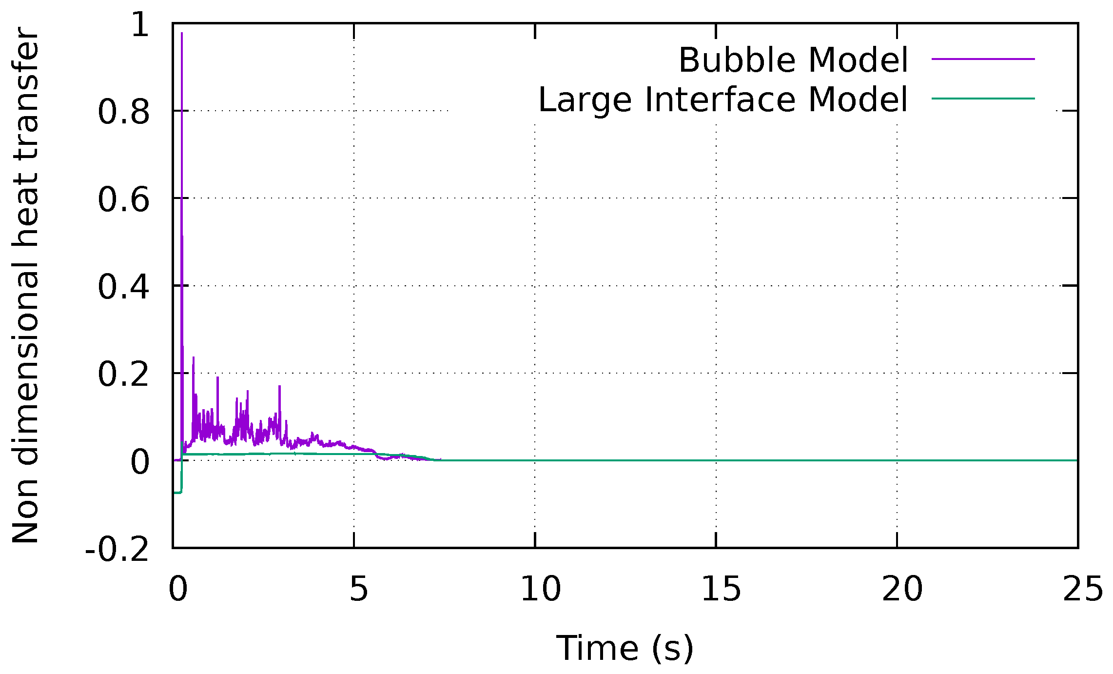
It should be noted that the heat transfer through large interfaces is much smaller than the heat transfer computed with the subgrid models, as shown in Figure 2.
If a dispersed model is chosen, the bubble model is used if the gas volume fraction is small in the cell, otherwise the droplet model is used (see Equation (25)). Table 1 summarises the subgrid models used by the GLIM.
Bubble model i f   α l < 0.4 Droplet model i f   α l > 0.6 Interpolation between the bubble and the droplet model i f   0.4 < α l < 0.6

2.4.1. Interfacial Momentum Transfer

If α l > 0.6 , liquid/bubble interactions are considered, and the drag force model of Ishii [17] for bubbles is used. If α l < 0.4 , gas/droplet interactions and the drag force model of Wen and Yu [31] for droplets are used. In this model, the drag coefficient C D depends on the Reynolds number for the gas R e g and on α g . For 0.4 < α l < 0.6 , it is considered that the cell contains both bubbles and droplets, and an interpolation of the two models is used to model the two types of interactions.
The lift force and the added mass force are neglected for droplets. Consequently, they are computed in the GLIM as
I g L / A = I l L / A = 0 i f α l < 0.5 I b , g L / A i f α l > 0.6 0.5 α g 0.1 I b , g L / A e l s e
I g L / A represents the interfacial lift or added mass term for the gas field. I b , g L / A is the interfacial lift or added mass term using a bubble model for the gas field, that is to say, the lift force of Tomiyama [18] or the added mass of Zuber [19].

2.4.2. Interfacial Enthalpy Transfer

In each cell, a droplet model, a bubble model, or a linear interpolation of the two models is used depending on the liquid fraction α l . The interpolation is given by Equation (27).
Π k = Π k , d r o p l e t i f   α l < 0.4 Π k , b u b b l e i f   α l > 0.6 α l 0.4 0.2 Π k , b u b b l e + 0.6 α l 0.2 Π k , d r o p l e t e l s e
Π k , b u b b l e is the enthalpy transfer for the field k using a bubble model. These models were described in Section 2.3.2, and are listed in Table 1.
Π k , d r o p l e t represents the enthalpy transfer for the field k using a droplet model. The enthalpy transfer for the gas is given in Equation (28). The enthalpy transfer for the liquid is given in Equation (29) [32].
Π g , d r o p l e t = 6 α l N u g λ g d d 2 ( T l T g )
d d is the droplet diameter (constant equal to 1 mm in the study). N u g is the Nusselt number for the gas, computed using the Ranz–Marshall correlation.
Π l , d r o p l e t = 6 α l N u g λ g d d 2 ( T l T g ) 6 α l S h . D d d 2 ( ρ s a t y v a p ρ g ) h f g
Sh is the Sherwood number calculated with the correlation of Frossling S h = 2 + 0.56 R e 1 / 2 S c 1 / 3 , with S c = μ g ρ g D being the Schmidt number. D is the coefficient of diffusion of the vapour in the gas mixture. y v a p is the mass fraction of vapour in the gas mixture. Finally, h f g is the latent enthalpy of vaporisation.
Table 1. Summary of the models used by the GLIM with dispersed models.
Interfacial TermModel for BubblesModel for Droplets
Drag force I k D [17][31]
Lift force I k L [18]0
Added mass force I k A [19]0
Enthalpy for the liquid Π l [20,33][32]
Enthalpy for the gas Π g Return to saturation[32]

3. Saury’s Experiments

3.1. The Experimental Facility

The principle of the experiment is explained in Section 1.1. At the start of the experiment, the flash chamber and the vacuum chamber are connected, which leads to the flashing of the liquid water. The flash chamber is filmed (this gives qualitative results) and the temperature of the liquid is measured during the experiment. Figure 3 is a schematic drawing of the flash chamber. It is a 195 mm high cylinder, with a 120 mm diameter, initially filled with 15 mm of liquid water. The valve is a 40 mm wide cylinder, connected to the side of the flash chamber.
During their Ph.D., Saury conducted over a hundred experiments. In this paper, seven of these experiments will be simulated, which are defined by the initial temperature of the liquid film and by the initial pressure in the vacuum chamber. The results of the experiments (P = 50 mbar, T 0 = 34 C), (P = 50 mbar, T 0 = 40 C), (P = 50 mbar, T 0 = 50 C), (P = 50 mbar, T 0 = 60 C), (P = 50 mbar, T 0 = 74 C), (P = 100 mbar, T 0 = 74 C), (P = 200 mbar, T 0 = 74 C) will be presented.

3.2. Mesh, Initial Conditions and Boundary Conditions

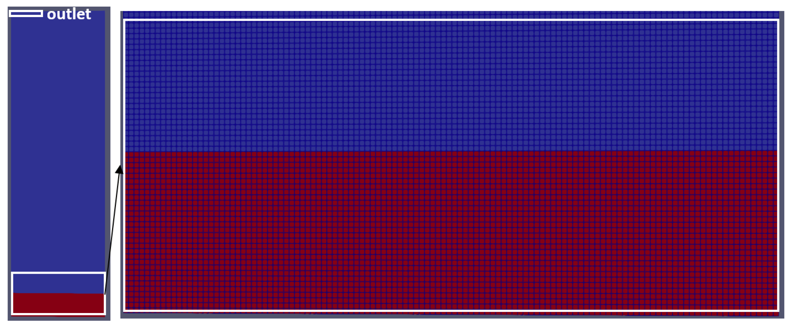
A 2D axisymmetric mesh is used to model the flash chamber. It represents a slice of 2° of the cylindrical chamber. The chamber was divided in 46,800 hexahedra with a size of 0.5 × 0.5 mm. Figure 4 shows the mesh of the experimental facility. The red part represents the initial water film with a height of 15 mm, while the blue part represents the initial gas region.
A preliminary mesh sensitivity study was conducted on the evolution of the liquid temperature over time using an Euler–Euler liquid/bubble model. It showed that a 3D mesh with a valve connected to the side was equivalent to a 2D axisymmetric mesh connected to a valve of the same surface (approximately 5000 mm 2 ) at its top. Furthermore, the mesh convergence was validated for coarser meshes than the one used. It was decided to use the fine mesh because the computational time was reasonable (less than 3 days with 10 processors), and the finer mesh gave better images. Mesh sensitivity is discussed in Appendix A.
The initial conditions of the experiment were respected: the chamber is initially at atmospheric pressure and filled with 15 mm of preheated liquid water. During the experiments of Saury, the air temperature and the vapour fraction were not measured. In the numerical simulations, it is assumed that the air is initially at the same temperature as the water. The initial air temperature is not very important and should not affect the results. It was also arbitrarily assumed that the initial mass fraction of vapour is 1%.
As for the boundary conditions, the walls were considered adiabatic. It was not possible to set a simple Dirichlet condition at 50 mbar for the outlet because of numerical issues caused by the pressure gradient. Consequently, a ramp from 1 bar to 50 mbar in 0.25 s was applied ( P o u t l e t = 100,000 100 , 000 5000 0.25 t (Pa) for t < 0.25 s). An adaptative time step was used with values of 1 and 10 set for the maximum Courant and Fourier numbers, respectively, for both the liquid and gas phases. This leads to time steps close to 10 3 s during most of the simulation.

4. Results and Discussion

In this section, qualitative comparisons between the pictures of the flash chamber taken during the experiment and CFD results postprocessed with the ParaView software (version 5.10.0) [35] will be presented. In a second subsection, the evolution of the temperature over time measured experimentally is compared to the numerical results.

4.1. Qualitative Results

Saury filmed the flash chamber during their experiment and provided pictures of the chamber in their Ph.D. thesis, which allows a comparison between the numerical results and their experiments.
Figure 5 shows the initial and final states (after five minutes) of the flash chamber in the experiment (top), and with the liquid/bubble model (bottom). In the experiment, the height of the liquid film does not vary significantly between the beginning and the end of the experiment. The liquid/bubble model, however, predicts that almost all the liquid disappeared during the simulation. The analysis of the numerical results reveals that most of the liquid water was not evaporated during the experiment but vacuumed. This is caused by the wrong modelling of the interfacial forces, especially the drag force by the liquid/bubble model. During the experiment, the quick bubble nucleation causes an explosion of the liquid film into droplets. The liquid/bubble approach can correctly model the explosion of the liquid film. However, this model only considers a continuous liquid and subgrid bubbles instead of a continuous gas and sub-grid droplets in the droplet region. Consequently, in the droplet region where the liquid fraction is low, the interfacial area is significantly overestimated ( A i = 6 α g d b ), and the drag force applied by the gas on the liquid is also overestimated, which explains the vacuuming of the liquid.
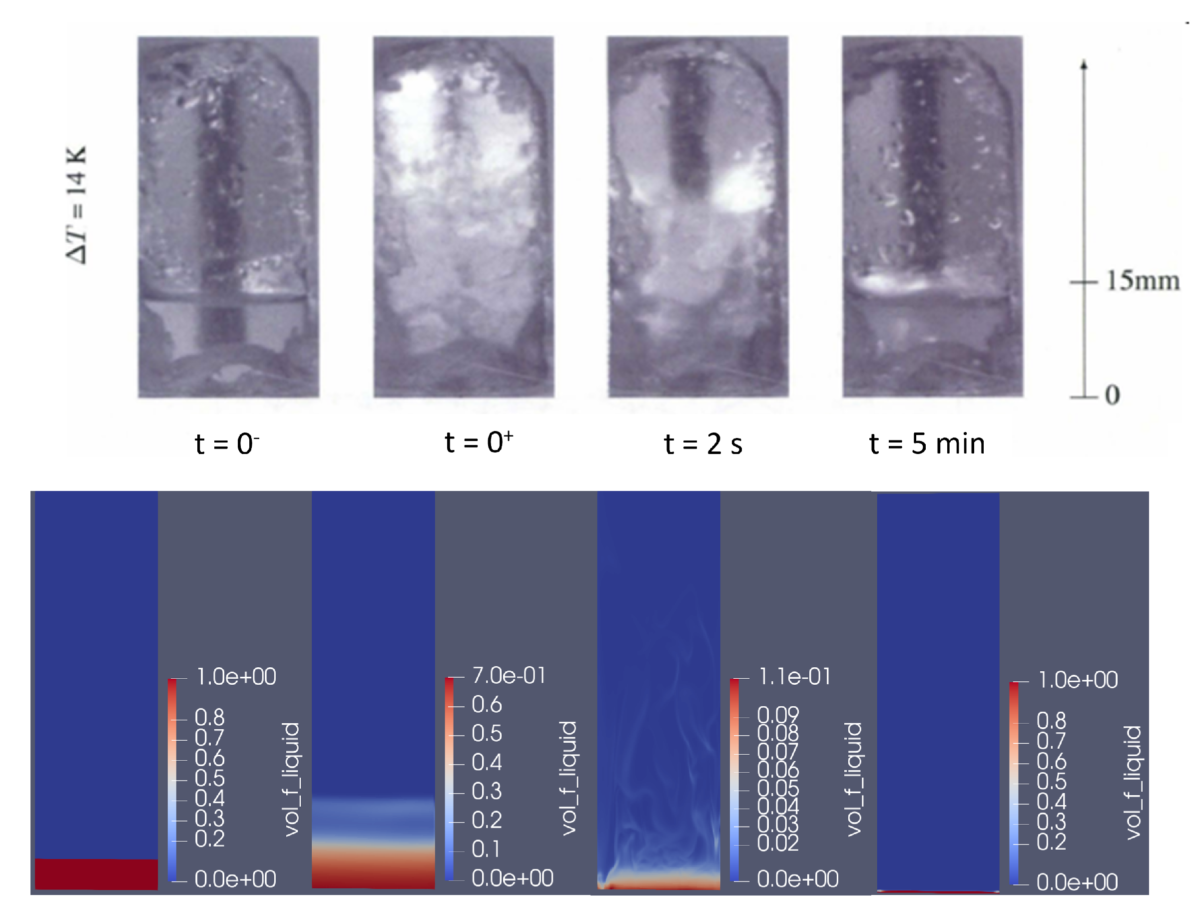
Figure 6 shows the comparison between four photographs of Saury’s experiments and the results with the GLIM for T 0 = 50 C. The first picture is taken before the experiment ( t = 0 s), the second just after the experiment begins ( t = 0 + s), the third after 2 s of experiment, and the last one after the final state is reached (five minutes).
Qualitatively, the GLIM shows a good agreement with the experiment. In the second picture, it predicts the explosion of the liquid film into a droplet film which occupies twice the initial volume. In the third picture, at t = 2 s, it shows a liquid film with bubbles at the bottom of the chamber below a droplet film. In the final state, the GLIM finds a liquid film with the same height as initially, like in the experiment.

4.2. Quantitative Results

Since the liquid/bubble model could not qualitatively predict the experiments correctly, only the results of the GLIM will be presented in this part. The evolution of the temperature over time will be compared with the experimental values. Extrapolating the evaporated mass from the liquid temperature (Equation (2)), the evaporated mass of liquid over time is also presented.
To measure the temperature of the water, Saury used three thermocouples placed at different heights. He found that the liquid temperature measured by the different thermocouples was very close (with more oscillations for the thermocouples placed initially in the air above the liquid). These measures will be compared to the average temperature of the liquid defined as T l = I = 0 N c e l l s ( α l I ρ l I c p , l I V I T l I ) I = 0 N c e l l s ( α l I ρ l I c p , l I V I ) , with N c e l l s as the number of cells and V I as the volume of cell I.

4.2.1. Evolution of the Temperature over Time

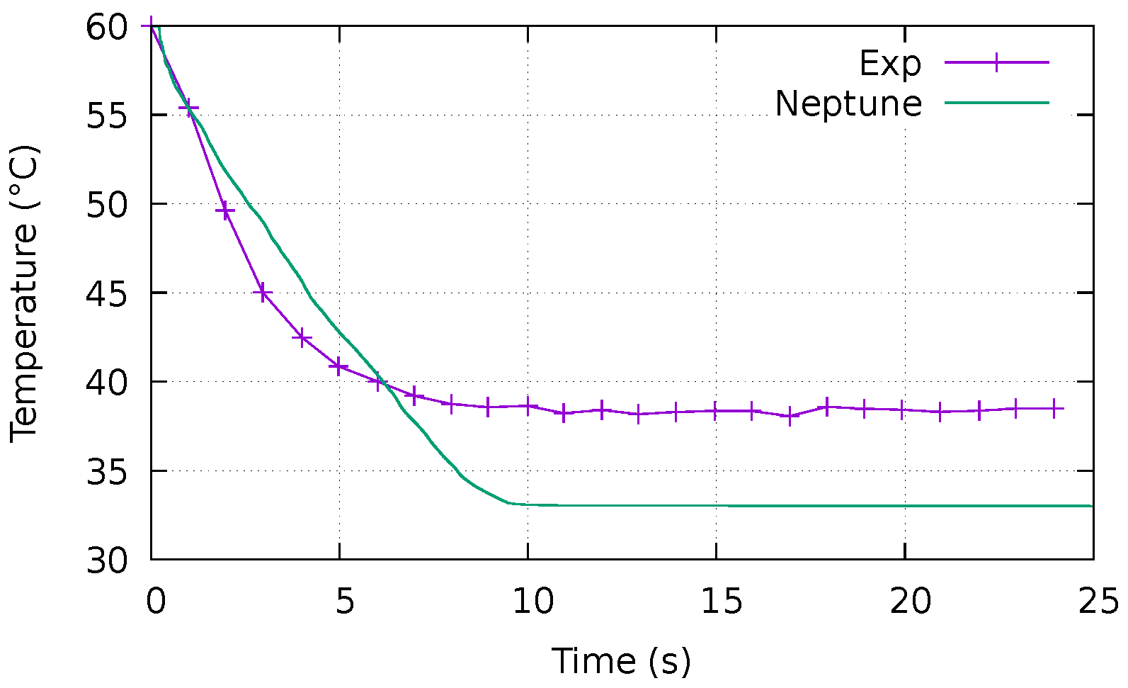
Figure 7 shows the evolution of the temperature over time and compares the experimental results (purple points) with the Neptune simulation (green). Surprisingly, the code and the experiment find a different asymptotic temperature (with more than 4 C difference), while the asymptotic temperature is supposed to be the saturation temperature at the asymptotic pressure ( T e = T s a t ( P f ) ) , that is to say 33 C for a final pressure of 50 mbar. That asymptotic pressure is correctly predicted by neptune_cfd, but not by the experiment.
The reason for that is that the vaporisation of the liquid leads to an increase in the gas pressure in the vacuum chamber, and consequently, to an increase in the saturation temperature. Hence, a high initial superheat leads to an important vaporisation, and thus, to a higher asymptotic temperature.
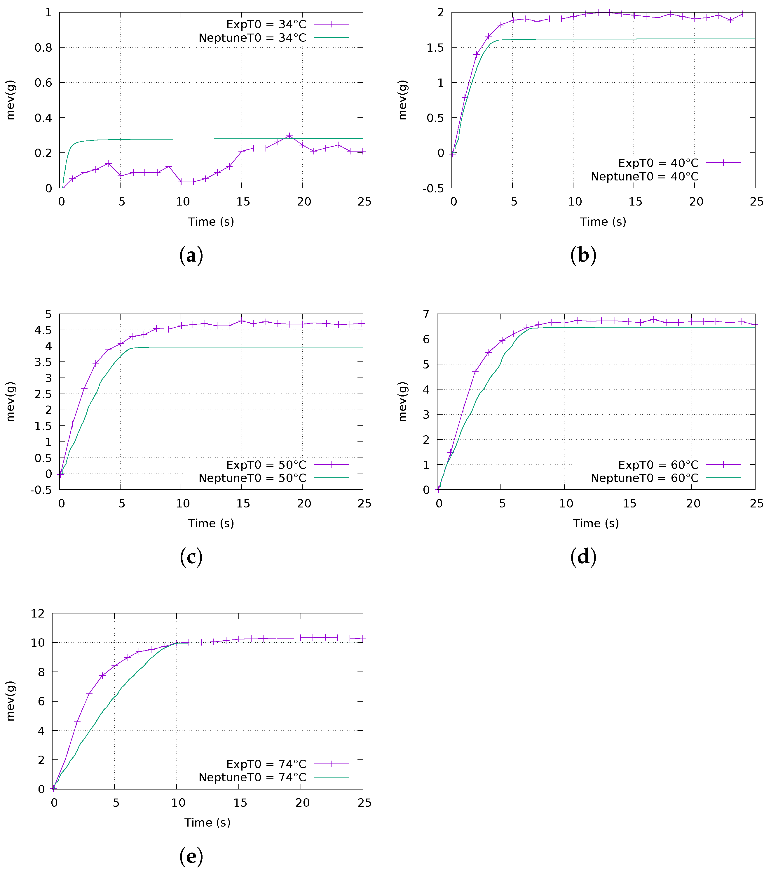
Using the experimental results on the evaporated mass of water, this difference can be quantified. For instance, for T 0 = 60 C, approximately 6.8 g of liquid evaporates during the experiment (Figure 8d), that is to say, Δ n = 0.38 mol. Assuming that the temperature in the vacuum chamber does not vary significantly, the ideal gas law (Equation (30)) gives P f = 65 mbar for T 0 = 60 C.
Δ P = R T Δ n V
The saturation temperature at P f = 65 mbar is 37.6 C, which is close to the asymptotic temperature found experimentally (Figure 7). Table 2 gives the final pressure and the final saturation temperature for the five experiments considered, using the ideal gas law. From now on, the outlet pressure P o u t is set using Table 2 instead of setting P o u t = 50 mbar.
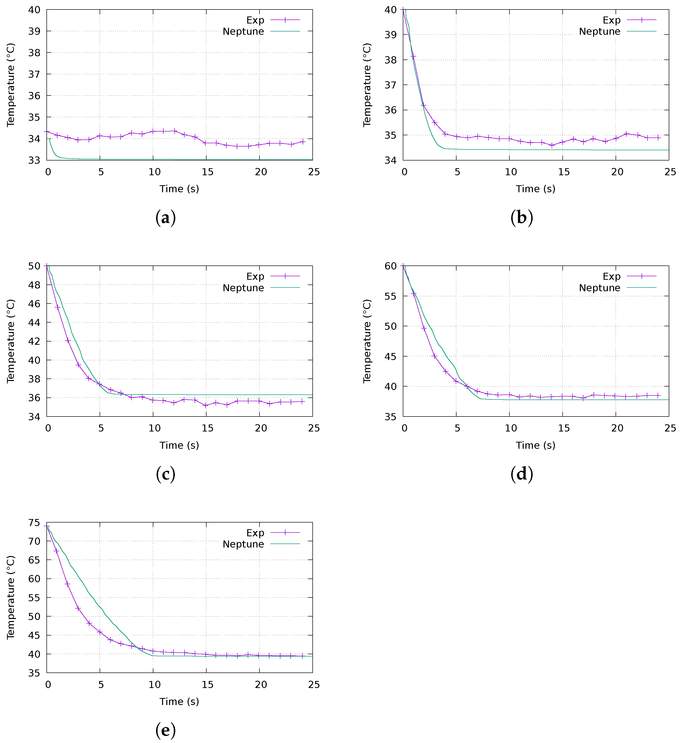
The results obtained after the pressure correction are given in Figure 9a–e. The simulations and the experiments now find similar asymptotic temperatures. The small differences in the asymptotic temperature are caused by:
1.
Experimental uncertainties on the temperature ( ± 0.5 C according to Saury [1]);
2.
Errors during the digitisation of the experimental results from the graphs given by Saury ( ± 0.5 C, particularly visible in Figure 9a);
3.
Computation of the asymptotic pressure with the ideal gas law (the error is difficult to quantify);
4.
Finally, Saury [1] explained that some experimental errors might come from the measurement of the liquid height, and affect the results by a few percent.
As for the transient regime, the numerically predicted evolution of the temperature over time is overall very close to the experimental temperature. However, Neptune tends to predict a slower decrease in temperature over time, especially for high superheats, and slightly overestimates the flashing time defined by Miyatake [7]. A sensitivity study on the bubble diameter revealed that this small difference is not a consequence of the choice of a bubble diameter of 1 mm. Hence, the small inaccuracy might be caused by the interfacial enthalpy transfer model.

4.2.2. Evolution of the Evaporated Mass over Time

To estimate the evaporated mass, Saury used m e v = ρ l A H ( 1 exp ( c p h f g ( T 0 T ) ) (Section 2). In practice, ρ l , c p and h f g vary slightly with the temperature. Therefore, the evaporated mass was extrapolated from the values of these properties at T 0 using the same formula and tables as Saury: the Regnault formula for the latent heat ( h f g = 3327 2.901 T kJ/kg, [36]), c p , l = 4.189 kJ/kg/K [37], and ρ l = 1.5211 × 10 5 T 3 5.8302 × 10 3 T 2 + 1.5372 × 10 2 T + 1000 kg/ m 3 with T in Celsius [37]. The physical properties for the five initial temperatures are given in Table 3.
The evaporated mass is almost proportional to the temperature; consequently, the conclusions are the same as in the previous section: the GLIM predicts a slightly slower increase in the evaporated mass over time, but the asymptotic evaporated mass is almost the same.
To assess whether the GLIM can also accurately predict the evaporated mass for higher pressures, two other flashing experiments were simulated. These experiments were also conducted by Saury using the same experimental facility:
1.
In one experiment, the initial pressure in the vacuum chamber is P = 100 mbar and the initial temperature is T 0 = 60 C, which represents a 14 C superheat;
2.
In the other experiment, the initial pressure is P = 200 mbar and the initial temperature is T 0 = 74 C, which also represents a 14 C superheat.
It should be noted that the pressure increase caused by the flashing can be neglected in these two cases because the pressures are higher. Figure 10a,b show the evaporated mass of liquid over time. The numerical results are in excellent agreement with the experiment, which shows that the GLIM is also valid for higher sub-atmospheric pressures.

4.3. Boiling at the Interface during the Second Stage

According to Miyatake [7], the flashing of a water film can be split into two stages. A first stage where the NEF rapidly decreases because boiling takes place at the bulk of the liquid, and a second stage where the decrease in the NEF is slower because boiling only takes place at the interface between the liquid and the gas (Figure 11).
The GLIM model used in neptune_cfd correctly predicts the existence of these two stages, and thus, it is possible to draw conclusions from the results of the numerical simulations.
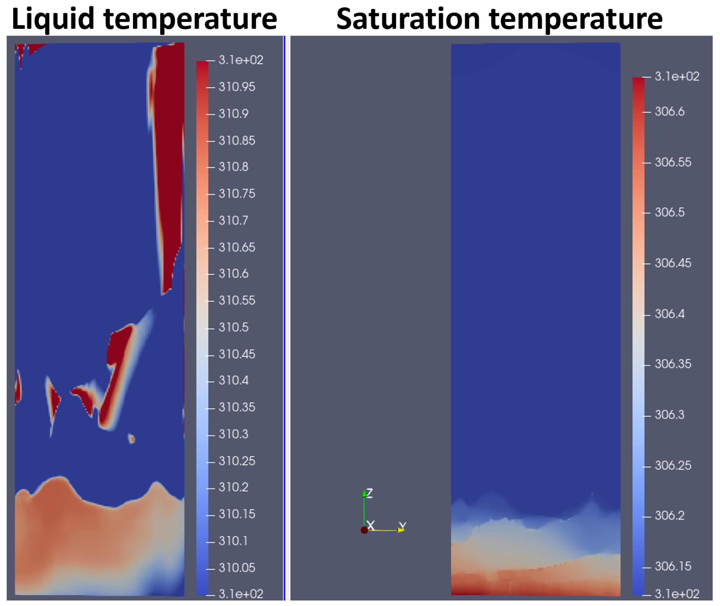
Figure 12 shows the temperature of the water and the saturation temperature in the flash chamber, for T 0 = 50 C. These views were taken at t = 10 s during the second stage. The left picture shows that the temperature of the liquid is higher near the interface—up to 0.5 C hotter. This is caused by the bulk boiling during the first stage, which leads to an important decrease in the temperature at the bulk of the water film. Additionally, the right picture shows that the saturation temperature is smaller at the interface (typically 0.5 C smaller) because of the weight of the water column. These two phenomena lead to a higher superheat Δ T = T l T s a t at the interface (typically 1 C higher in the experiments of Saury), and explain why boiling only happens at the interface when the temperature of the liquid is close to the saturation temperature.

5. Conclusions

In this paper, it was shown that the flashing of a water film could not be simulated using a simple liquid/bubble model, because the interfacial area between the liquid and the vapour is heavily overestimated in the droplet region (by a factor 10–100). As a consequence, the interfacial force of the gas on the liquid is overestimated and the liquid film is vacuumed. Using the recent GLIM model, it was possible to determine, in each cell, which of the liquid/bubble model or the gas/droplet model was the most appropriate, leading to very nice qualitative results.
Quantitatively, it was shown that the pressure increase caused by the evaporated mass of water during the experiments of Saury was not negligible at 50 mbar for a vacuum chamber of 0.6 m 3 , and leads to asymptotic pressures higher than 50 mbar. After correcting the pressure at the outlet, the prediction of the temperature over time and the prediction of the evaporated mass over time were in very good agreement with the experimental results. At any time, the difference on the liquid temperature between the experiment and the numerical simulations is smaller than 4 C (10%), except in the case (P = 50 mbar, T0 = 74 C), where the difference can go up to 10 C (20%) during the first ten seconds of the experiment. In the steady state ( t > 10 s), the error on the asymptotic temperature is smaller than 1 C in the seven cases studied.
Using CFD results, it was shown that the liquid superheat is more important near the interface, which explains why the second stage of the flashing of a water film, defined by Miyatake, involves boiling at the interface between the water film and the gas when the liquid superheat is small.
To obtain even better macroscopic results (such as the evolution of the average temperature over time), the Berne coefficient C b e r n e , developed for high-pressure flashing and involved in the enthalpy transfer for superheated liquids, needs to be increased for sub-atmospheric flashing with a large superheat. Finally, to improve the local results, one way would be to use a more refined mesh and an interface capturing approach, instead of the LIM, to consider surface tension effects. Such an approach would model the bubbles more accurately, but also have a greater computational cost.

Author Contributions

C.L.: Conceptualisation, Investigation, Methodology, Validation, Visualisation, Writing—Original Draft, Review and Editing. S.M.: Supervision, Writing—Review and Editing. D.C.: Supervision, Writing—Review and Editing. S.V.: Supervision, Writing—Review and Editing. All authors have read and agreed to the published version of the manuscript.

Funding

This work was financially supported by EDF and MSME (Laboratoire Modélisation et Simulation Multi Echelle). The neptune_cfd code is financially supported by EDF, Commissariat à l’Energie Atomique et aux Energies Alternatives (CEA), Institut de Radioprotection et de Sûreté Nucléaire (IRSN), and Framatome.

Data Availability Statement

All the data used in this article are publicly available in Saury’s Ph.D Thesis (https://hal.science/tel-03001965/).

Acknowledgments

This work was conducted within the framework of the PRETING project, and financially supported by EDF. The neptune_cfd code is being developed in the framework of the NEPTUNE project, financially supported by EDF, Commissariat à l’Energie Atomique et aux Energies Alternatives (CEA), Institut de Radioprotection et de Sûreté Nucléaire (IRSN), and Framatome.

Conflicts of Interest

The authors declare that they have no known competing financial interests or personal relationships that could have appeared to influence the work reported in this paper.

Appendix A. Mesh Sensitivity

With an extremely fine mesh ( Δ x = 1 μ m for example), all the bubbles and droplets would be modelled with the large interface model. Nevertheless, it is not realistic to use such a fine mesh because the computational domain would require over 10 10 cells, and the CFL requirement would lead to a time step of Δ t = 10 7 s. With coarser meshes, the small bubbles and droplets have to be represented with subgrid models. Therefore, the GLIM is by definition sensitive to the mesh.
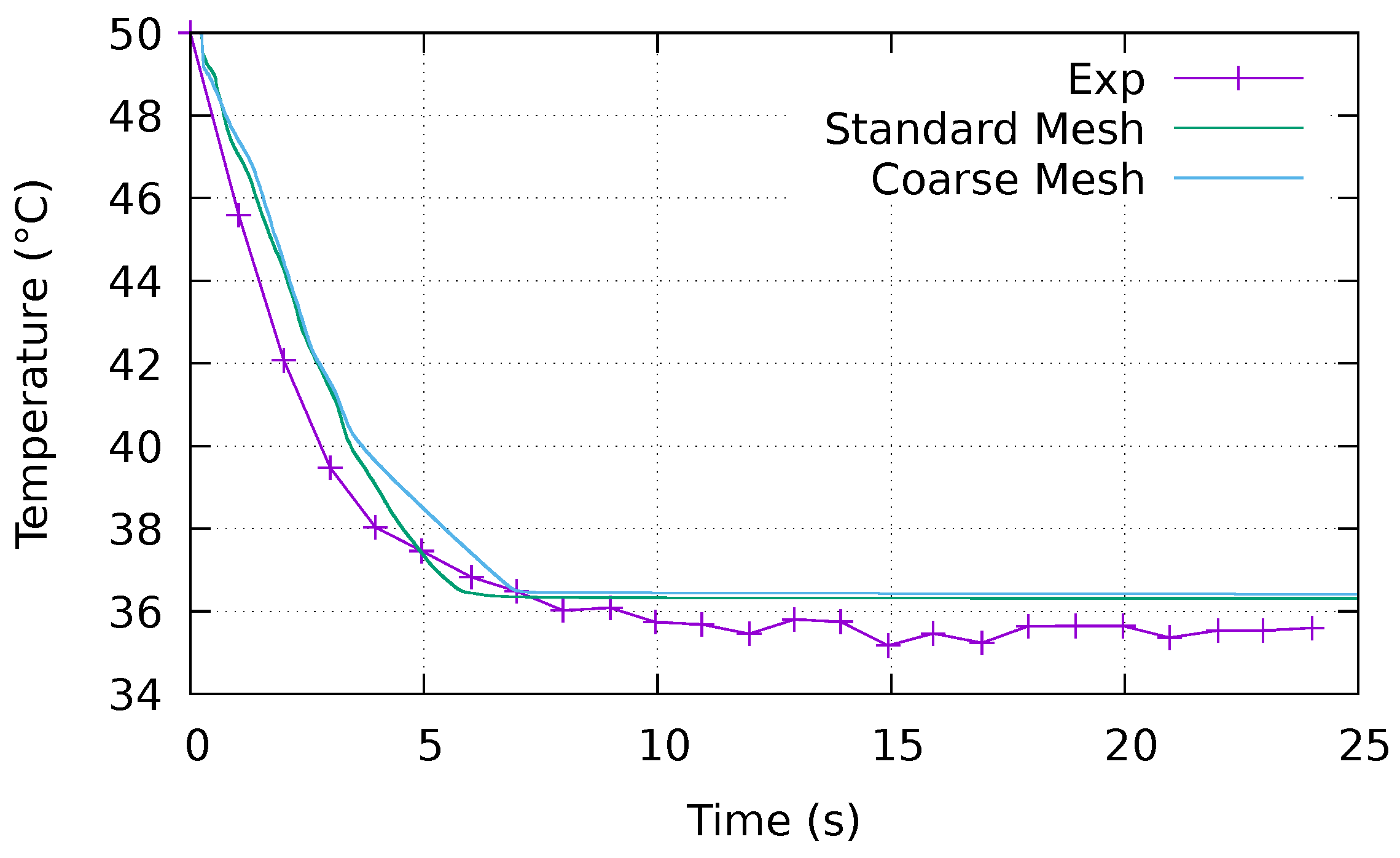
That being said, Figure 1 shows that most of the heat transfer comes from the bubble model, and not from the LIM in this study. This explains why the evolution of the temperature over time is not very sensitive to the mesh, as shown in Figure A1. The decrease in the temperature during the first four seconds is almost the same. During this stage, the nucleation of very small bubbles and the explosion of the liquid film is handled by subgrid models. A small difference between the two meshes can be observed between four and seven seconds. During this second stage, larger bubbles can be observed. These bubbles are modelled with the LIM with the standard mesh, while they are modelled with a subgrid bubble model with the coarse mesh. Nonetheless, the difference between the two meshes is only 1 C during the second stage, and both models converge toward the asymptotic temperature. Therefore, the results presented in this article are not very sensitive to the mesh.
Figure A1. Evolution of the temperature over time for (P = 50 mbar, T 0 = 50 C). The standard mesh is presented in Section 3.2 and the size of the cells is 0.5 × 0.5 mm. The size of the cells of the coarse mesh is 1 × 1 mm. This figure shows that the evolution of the temperature over time is almost the same with both meshes.
Fluids 08 00143 g0a1

References

  1. Saury, D. Etude Expérimentale de l’Évaporation d’un Film d’Eau. Ph.D. Thesis, Université de Valenciennes et du Hainaut-Cambrésis, Valenciennes, France, 2003. [Google Scholar]
  2. Lv, H.; Wang, Y.; Wu, L.; Hu, Y. Numerical simulation and optimization of the flash chamber for multi-stage flash seawater desalination. Desalination 2019, 465, 69–78. [Google Scholar] [CrossRef]
  3. Woods, A.; Bloom, F.; Orloff, D. Modeling of flash evaporation I: Formulation of the mathematical model. Math. Comput. Model. 2000, 32, 1153–1169. [Google Scholar] [CrossRef]
  4. Mimouni, S.; Boucker, M.; Laviéville, J.; Guelfi, A.; Bestion, D. Modelling and computation of cavitation and boiling bubbly flows with the NEPTUNE_CFD code. Nucl. Eng. Des. 2008, 238, 680–692. [Google Scholar] [CrossRef]
  5. Narayanan, C. Numerical simulation of flashing using a pressure-based compressible multiphase approach and a thermodynamic cavitation model. Int. J. Multiph. Flow 2021, 135, 103511. [Google Scholar] [CrossRef]
  6. Hurisse, O.; Quibel, L. Simulations of water-vapor two-phase flows with non-condensable gas using a Noble-Able-Chemkin stiffened gas equation of state. Comput. Fluids 2022, 239, 105399. [Google Scholar] [CrossRef]
  7. Miyatake, O.; Murakami, K.; Kawata, Y. Fundamental experiments with flash evaporation. Heat Transf.-Jpn. Res. 1973, 2, 89–100. [Google Scholar]
  8. Gopalakrishna, S.; Purushothaman, V.; Lior, N. An experimental study of flash evaporation from liquid pools. Desalination 1987, 65, 139–151. [Google Scholar] [CrossRef]
  9. Augusto, C.; Ribeiro, J.; Gaspar, A.; Costa, J. Low-pressure-vaporization of free water—Characterization of the boiling regimes. Int. J. Therm. Sci. 2014, 77, 19–26. [Google Scholar] [CrossRef]
  10. Wang, C.; Xu, R.; Chen, X.; Jiang, P.; Liu, B. Study on water flash evaporation under reduced pressure. Int. J. Heat Mass Transf. 2019, 131, 31–40. [Google Scholar] [CrossRef]
  11. Enoki, K.; Ono, M.; Okawa, T.; Kristiawan, B.; Wijayanta, A.T. Water flow boiling heat transfer in vertical minichannel. Exp. Therm. Fluid Sci. 2020, 117, 110147. [Google Scholar] [CrossRef]
  12. Ishii, M. Thermo-fluid dynamic, theory of two phase. In Collection de la Direction des Etudes et Recherches d’Electricité de France; Springer: Berlin/Heidelberg, Germany, 1975. [Google Scholar]
  13. Delhaye, J.M.; Giot, M. Thermal-Hydraulics of Two-Phase Systems for Industrial Design and Nuclear Engineering; Hemisphere: New York, NY, USA, 1981. [Google Scholar]
  14. Guelfi, A. NEPTUNE—A new software platform for advanced nuclear thermal hydraulics. Nucl. Sci. Eng. 2007, 156, 281–324. [Google Scholar] [CrossRef]
  15. Mimouni, S. Modeling and computation of cavitation and boiling bubbly flows with the NEPTUNE_CFD code. Nucl. Sci. Eng. 2008, 156, 281–324. [Google Scholar]
  16. Speziale, C.G.; Sarkar, S.; Gatski, T.B. Modelling the pressure–strain correlation of turbulence: An invariant dynamical systems approach. J. Fluid Mech. 1991, 227, 245–272. [Google Scholar] [CrossRef]
  17. Ishii, M.; Zuber, N. Drag coefficient and relative velocity in bubbly, droplet or particulate flows. AIChE J. 1979, 25, 843–855. [Google Scholar] [CrossRef]
  18. Tomiyama, A.; Tamai, H.; Zun, I.; Hosokawa, S. Transverse migration of single bubbles in simple shear flows. Chem. Eng. Sci. 2002, 57, 1849–1858. [Google Scholar] [CrossRef]
  19. Zuber, N. On the dispersed two-phase flow in the laminar flow regime. Chem. Eng. Sci. 1964, 19, 897–917. [Google Scholar] [CrossRef]
  20. Berne. Analyse Critique des Modèles d’Autovaporisation Utilisés dans le Calcul des Écoulements Diphasiques en Conduites. Ph.D. Thesis, Ecole Centrale Paris, Gif-sur-Yvette, France, 1983. [Google Scholar]
  21. Mérigoux, N.; Lavieville, J.; Mimouni, S.; Guingo, M.; Baudry, C. A generalized large interface to dispersed bubbly flow approach to model two-phase flows in nuclear power plant. In Proceedings of the 6th Workshop on Computational Fluid Dynamics for Nuclear Reactor Safety (CFD4NRS-6), Cambridge, MA, USA, 13–15 September 2016. [Google Scholar]
  22. Mer, S.; Praud, O.; Neau, H.; Merigoux, N.; Magnaudet, J.; Roig, V. The emptying of a bottle as a test case for assessing interfacial momentum exchange models for Euler–Euler simulations of multi-scale gas-liquid flows. Int. J. Multiph. Flow 2018, 106, 109–124. [Google Scholar] [CrossRef] [Green Version]
  23. Davy, G.; Reyssat, E.; Vincent, S.; Mimouni, S. Euler–Euler simulations of condensing two-phase flows in mini-channel: Combination of a sub-grid approach and an interface capturing approach. Int. J. Multiph. Flow 2022, 149, 103964. [Google Scholar] [CrossRef]
  24. Honda, H.; Wijayanta, A.; Takata, N. Condensation of R407C in a horizontal microfin tube. Int. J. Refrig. 2005, 28, 203–211. [Google Scholar] [CrossRef]
  25. Griffith, P.; Wallis, G.B. Two-Phase Slug Flow. J. Heat Transf. 1961, 83, 307–318. [Google Scholar] [CrossRef]
  26. Taitel, Y.; Bornea, D.; Dukler, A.E. Modelling flow pattern transitions for steady upward gas-liquid flow in vertical tubes. AIChE J. 1980, 26, 345. [Google Scholar] [CrossRef]
  27. Murzyn, F.; Chanson, H. Free-Surface Fluctuations in Hydraulic Jumps: Experimental Observations. Exp. Therm. Fluid Sci. 2009, 33, 1055–1064. [Google Scholar] [CrossRef] [Green Version]
  28. Mimouni, S.; Foissac, A.; Lavieville, J. CFD modelling of wall steam condensation by a two-phase flow approach. Nucl. Eng. Des. 2011, 241, 4445–4455. [Google Scholar] [CrossRef] [Green Version]
  29. Loiseau, C.; Mimouni, S.; Studer, E. Numerical simulation of wall condensation and spray using the MISTRA experiments. Nucl. Eng. Des. 2023, 402, 112111. [Google Scholar] [CrossRef]
  30. Coste, P. A Large Interface Model for two-phase CFD. Nucl. Eng. Des. 2013, 255, 38–50. [Google Scholar] [CrossRef]
  31. Wen, C.; Yu, Y. Mechanics of Fluidization. Chem. Eng. Prog. 1966, 162, 100–111. [Google Scholar]
  32. Mimouni, S.; Lamy, J.S.; Lavieville, J.; Guieu, S.; Martin, M. Modelling of sprays in containment applications with A CMFD code. Nucl. Eng. Des. 2010, 240, 2260–2270. [Google Scholar] [CrossRef] [Green Version]
  33. Manon, E. Contribution à l’Analyse et à la Modélisation Locale des Écoulements Bouillants Sous-Saturés dans les Conditions des Réacteurs à Eau sous Pression. Ph.D. Thesis, Ecole Centrale Paris, Gif-sur-Yvette, France, 2000. [Google Scholar]
  34. Saury, D.; Harmand, S.; Siroux, M. Experimental study of flash evaporation of a water film. Int. J. Heat Mass Transf. 2002, 45, 3447–3457. [Google Scholar] [CrossRef]
  35. Ahrens, J.; Geveci, B.; Law, C. 36-ParaView: An end-user tool for large-data visualization. Vis. Handb. 2005, 717, 50038-1. [Google Scholar]
  36. Bruhat, G. Cours de Physique Générale, 6th ed.; Masson: Issy-les-Moulineaux, France, 1968. [Google Scholar]
  37. Massart, F. Aide Mémoire du Thermicien; Elsevier: Amsterdam, The Netherlands, 1997. [Google Scholar]
Figure 1. Schematic drawing of the three situations considered in the GLIM. The left picture shows a cell with four gas bubbles, which should be solved using the liquid/bubble model. The middle picture shows a gas bubble in a liquid. The diameter of the bubble is larger than the size of a cell, and the large interface model (LIM) should be used. Finally, the right picture shows a cell with four droplets. It should be solved using the gas/droplet model.
Fluids 08 00143 g001
Figure 2. Evolution of the non-dimensional heat transfer between the gas and the liquid over time for the bubble model and for the LIM in the case ( P 0 = 50 mbar, T 0 = 50 C). This figure shows that the contribution of the bubble model in the heat and mass transfer is significantly higher than the contribution of the LIM in the GLIM.
Fluids 08 00143 g002
Figure 3. Schematic drawing of the flash chamber by Saury [34]. The unit of length is the millimetre. Reprinted from [34], Elsevier, Copyright 2023 with permission.
Fluids 08 00143 g003
Figure 4. Mesh of the flash chamber. The red phase represents the initial liquid film, and the blue phase represents the gas. The left picture shows the total mesh. The right picture is a zoom on the liquid film to show the size of the cells.
Fluids 08 00143 g004
Figure 5. Qualitative comparison of the flash chamber between the experiment (top from [1] D. Saury, Copyright 2023 with permission), and the liquid/bubble model for ( P 0 = 50 mbar, T 0 = 50 C) (bottom). This figure shows that almost all of the water is vacuumed from the chamber with the bubble model, which does not happen in the experiment.
Fluids 08 00143 g005
Figure 6. Qualitative comparison between the experiment (top, from [1] D. Saury, Copyright 2023 with permission), and the GLIM for T 0 = 50 C (bottom). This figure shows a good qualitative agreement between the GLIM simulation and the experiment.
Fluids 08 00143 g006
Figure 7. Evolution of the temperature over time for ( P = 50 mbar, T 0 = 60 C) with the GLIM. This figure shows that the asymptotic temperature predicted by Neptune is significantly smaller than the experimental temperature.
Fluids 08 00143 g007
Figure 8. Evolution of the evaporated mass over time for T0 = 34 C, T0 = 40 C, T0 = 50 C, T0 = 60 C, and T0 = 74 C at P = 50 mbar with the GLIM. (a) Evaporated mass over time for ( P = 50 mbar, T 0 = 34 C) using the GLIM. (b) Evaporated mass over time for ( P = 50 mbar, T 0 = 40 C) using the GLIM. (c) Evaporated mass over time for ( P = 50 mbar, T 0 = 50 C) using the GLIM. (d) Evaporated mass over time for ( P = 50 mbar, T 0 = 60 C) using the GLIM. (e) Evaporated mass over time for ( P = 50 mbar, T 0 = 74 C) using the GLIM.
Fluids 08 00143 g008
Figure 9. Evolution of the temperature over time for T0 = 34 C, T0 = 40 C, T0 = 50 C, T0 = 60 C, and T0 = 74 C at P = 50 mbar with the GLIM: (a) Temperature over time for ( P = 50 mbar, T 0 = 34 C) using the GLIM. (b) Temperature over time for ( P = 50 mbar, T 0 = 40 C) using the GLIM. (c) Temperature over time for ( P = 50 mbar, T 0 = 50 C) using the GLIM. (d) Temperature over time for ( P = 50 mbar, T 0 = 60 C) using the GLIM. (e) Temperature over time for ( P = 50 mbar, T 0 = 74 C) using the GLIM.
Fluids 08 00143 g009
Figure 10. Evolution of the evaporated mass over time for ( P = 100 mbar, T 0 = 60 C) and ( P = 200 mbar, T 0 = 74 C) with the GLIM. (a) Evaporated mass over time for P = 100 mbar and T0 = 60 C. (b) Evaporated mass over time for P = 200 mbar and T0 = 74 C.
Fluids 08 00143 g010
Figure 11. Evolution of the NEF over time ([1] D. Saury, Copyright 2023 with permission). The two asymptotic dashed lines represent the two steps of the flashing phenomenon, namely the bulk boiling and the surface boiling. t is defined as the flashing time.
Fluids 08 00143 g011
Figure 12. View of the temperature of the liquid (left) and of the saturation temperature in the flash chamber (right) in the flash chamber at t = 10 s, for ( P = 50 mbar, T 0 = 50 C). This figure shows that the liquid temperature is higher at the interface, and the saturation temperature is lower at the interface.
Fluids 08 00143 g012
Table 2. Evaporated mass and physical properties of the vapour at the end of the experiment.
T 0 ( C) m ev ( g ) n ev (mol) P f (mbar) T sat ( P f ) ( C)
340.20.0115033.0
4020.115434.3
504.50.256036.2
606.80.386537.6
7410.00.567139.0
Table 3. Physical properties of water at 34 C, 40 C, 50 C, 60 C, and 74 C.
T 0 ( C) ρ l (kg/m 3 ) h fg (kJ/kg)
34994.052433
40992.262419
50988.102390
60983.222360
74975.382320
Disclaimer/Publisher’s Note: The statements, opinions and data contained in all publications are solely those of the individual author(s) and contributor(s) and not of MDPI and/or the editor(s). MDPI and/or the editor(s) disclaim responsibility for any injury to people or property resulting from any ideas, methods, instructions or products referred to in the content.