1. Introduction
Temperature gradients can arise in a fluid as a result of the presence of internal heat sources. The density of heat sources can be constant, depending on one or several spatial coordinates, or can be a nonlinear function of the temperature. Examples include, but are not limited to, neutron irradiation in thermonuclear reactors [
1], biomass thermal conversion [
2,
3], and convection in the Earth’s mantle [
4]. These examples also represent multiphysics problems where different physical mechanisms are coupled. There are three different approaches to the solution of complex problems in science and engineering: (a) experimental studies, (b) numerical modeling, and (c) stability analysis. Stability theory is used in an attempt to answer the question: when and how does the given base flow become unstable? Tools and methods of stability analysis are varied, ranging from stochastic analysis [
5] to a deterministic approach [
6] based on Lyapunov theory [
7]. In the present paper we use a linear stability approach to analyze a convective flow in the region bounded by two vertical coaxial cylinders.
Hydrodynamic instability of a flow results in either a new laminar flow with more complicated structure (as for the case of the Taylor–Couette flow between two rotating cylinders [
8]) or a rapid transition to turbulence (examples include, but are not limited to, pipe Poiseuille flow [
9] or rapidly accelerated and decelerated pipe flows [
10]). In applications for aerodynamics (stability of a flight of an airplane) or for hydraulic engineering (waterhammer phenomenon in rapidly decelerating flows) instability should be avoided or, at least, controlled. There are applications, however, where instability is desirable. One example of such a situation is biomass thermal conversion [
2] where thermal instability results in more intensive mixing and, possibly, more efficient energy conversion. Our objective is the present paper is to analyze the factors that may enhance instability.
The linear stability of a convective flow in a plane vertical channel caused by internal heat sources with constant density is analyzed in [
11]. It is shown in [
11] that depending on the value of the Prandtl number, two types of instability exist: (a) shear instability and (b) buoyant instability. Similar results are obtained later in [
12]. The effect of different boundary conditions for the temperature on the stability characteristics is explored in [
13]. Stability analysis of convective flows with constant density of heat sources in cylindrical geometry is conducted in [
14,
15,
16]. The calculated linear stability characteristics are compared with experimental data in [
16] for the case of heat sources of constant density in a pipe. Reasonable agreement is found in terms of the form of unstable perturbation and critical values of the Grashof number. Linear stability of a combined flow caused by external pressure gradient, uniform volumetric heating, and different constant wall temperatures in a vertical fluid layer are analyzed in [
17]. Multiple local minima observed on the marginal stability curves facilitate instability.
As mentioned above, different forms of the distribution of heat sources are of interest in applications. One example is related to the flow where a light beam is passing through the fluid in such a way that all absorbed energy is released in the form of heat [
18]. In this case the density of heat sources is an exponential function of the transverse coordinate. Such a distribution of heat sources is recently analyzed in [
19] for the purpose of designing water-flow building facades with the objective to obtain solar energy. Other examples of flows with non-uniform density of heat sources are considered in [
20,
21,
22].
Identification and use of new sources of energy are crucial for the development of our society. One promising alternative to classical sources of energy is biomass thermal conversion [
23,
24,
25]. Since the problem includes different physical effects (chemical reactions, convection) and the corresponding models contain many parameters (see, for example, [
26]), numerical modeling can be time-consuming. Linear stability analysis can be used as an alternative to numerical or experimental investigations in an attempt to identify the factors that affect the conversion process. Linear stability analyses of chemically reacting fluid are conducted in [
27]. It is assumed in [
26,
27] that the density of internal heat sources is a nonlinear function of the temperature. This fact introduces an additional challenge for the base flow solution—the corresponding boundary value problem becomes nonlinear with one, two, or no solutions (depending on the value of the parameter that characterizes the thermal effect of the chemical reaction). Linear stability analysis is usually performed for the parameter range corresponding to two solutions. Thus, the “correct” base flow solution should be selected for stability analysis.
The study performed in the present paper is different from the other linear stability studies of a chemically reacting fluid in the following aspects: (a) bifurcation analysis is performed to identify the number of solutions of the nonlinear boundary value problem for the base flow temperature distribution and its structure; (b) the results from part (a) are used to choose the corresponding base flow solution for linear stability analysis; (c) convection is generated by two factors—internal heating of the fluid as a result of the chemical reaction and temperature difference between the walls; (d) it is found that the temperature gradient due to the difference between the wall’s temperatures is an additional destabilizing factor; (e) a new instability mode has been observed for
. The paper is organized as follows. Mathematical formulation of the problem is presented in
Section 2. Bifurcation analysis for the nonlinear boundary value problem is performed in
Section 3 with the objective to identify the structure and number of solutions in the parameter space. Results from
Section 3 are used to select the base flow solution. The linear stability problem for the base flow is formulated in
Section 4. Numerical results of linear stability calculations for different values of the parameters of the problem are presented in
Section 5. In addition, two cases are considered where the wall temperatures are either equal to zero or not.
2. Mathematical Formulation of the Problem
Consider a flow of a viscous incompressible fluid in the region
between two concentric cylinders (see
Figure 1). Linear stability analysis of the base flow (the base flow velocity distribution is shown in
Figure 1 in red) is performed in the paper. The system of cylindrical polar coordinates
with the origin at the axes of the cylinders is used to describe the flow. The following convention is used throughout: the variables with tildes are dimensional while the variables without tildes are dimensionless.
Convective flow in the annulus formed by the cylinders is caused by two factors: (a) different constant temperatures
of the walls
and
, respectively, that cause a temperature gradient in the radial direction and (b) heat release due to chemical reaction that takes place in the fluid. Internal heat sources generate convection in the vertical direction. Here
,
. The distribution of the density of the heat sources follows the Arrhenius’ law [
28]:
The notations are as follows:
E is the activation energy,
is the universal gas constant,
is a constant, and
is the absolute temperature. The dimensionless form of the system of the Navier–Stokes equations under the Boussinesq approximation is used in the analysis:
The Boussinesq approximation is explained in detail in many papers (see, for example, [
29,
30,
31,
32,
33]). The main assumptions are (a) non-uniformity of fluid density caused by changes in pressure is small and is neglected, (b) non-uniformity of density caused by non-uniform temperature distribution is assumed to be small, so that the density is given by
where
is a constant and
is the coefficient of the thermal expansion. The detailed derivation of the dimensionless form of Equations (
2)–(
4) is found elsewhere (see, for example, [
32]) and is not shown here for brevity. Here
is the velocity of the fluid,
T is the temperature,
p is the pressure, and
. To simplify the mathematical formulation of the source term we use the Frank-Kamenetskii transformation [
28]. The transformation consists of the following steps: (a) expand the exponent in a Taylor series in (
1) and (b) keep only the linear terms of the expansion. As a result, a more convenient form of the source term is obtained (see (
3)). Such a transformation is rather accurate for the range of parameters of interest in (
1), see [
28,
34].
Some chemical reactions taking place in a fluid lead to heat generation and to formation of a product which has density different from the density of a reagent. Changes in the density caused by the changes in temperature and concentration lead to convection in the reacting fluid. Different formulations of the problem are available depending on the type of a chemical reaction or on the relative role of the thermal effect of the reaction. If the thermal effect fo the reaction is large, one can neglect the dependence of internal heat generation from the concentration of the reagent. In this case, convection occurs due to internal heat sources distributed in the fluid in accordance with (
1). This is the assumption considered in the present paper.
To transform the system of the Navier–Stokes equations with convection to the dimensionless form we choose the following scales, respectively, for length,
, time,
, velocity,
, temperature,
, and pressure,
. Here
is the density of the fluid,
g is the acceleration due to gravity, and
is the viscosity of the fluid. The following dimensionless parameters are introduced: the Grashof number,
, the Prandtl number,
, and the Frank-Kamenetskii parameter,
, where
is the thermal diffusivity. The meaning of the dimensionless parameters is as follows. The Grashof number represents the ratio between the buoyancy force (due to non-uniformity in the temperature) and viscous force. The Prandtl number characterizes the properties of the fluid (the ratio of the viscosity and thermal conductivity). Finally, the Frank-Kamenetskii parameter represents internal heating of the fluid due to the chemical reaction that takes place in it. There exists a steady solution of (
2)–(
4) of the following structure:
The flow (
6) is known as the fully developed flow in the literature [
35]. It can be implemented in a middle portion of a sufficiently tall vertical annulus with a large aspect ratio. One example of the comparison of the linear stability characteristics with experimental data for aspect ratio of 38.6 is given in [
36] where it is shown, in particular, that the measured wavelegth of the cells is in good agreement with theoretical predictions obtained for an annulus of infinite length. Steady-state equations for the functions
,
, and
are obtained from (
2)–(
6) and have the form
where
.
The boundary conditions are
We assume that there are lids that cover the annulus at
so that
Nonlinearity in the boundary value problem (
7)–(
10) appears only in the heat Equation (
8). Bifurcation analysis performed in the next section shows that the number of solutions of the problem (
8) and (
9) for the temperature
depends on the value of the Frank-Kamenetskii parameter
F.
3. Bifurcation Analysis
Consider the boundary value problem
where
and
. Let us consider the auxiliary initial value problem (
11),
Acting in a similar way as in [
37,
38], the change of variables
,
reduces (
11), (
13) to the initial value problem
By calculations, the function
solves (
14) in the interval
, and thus the function
solves (
11), (
13) in the interval
.
Let
R be a fixed number in the interval
. Suppose that a function
is defined by (
15); then, the equation
defines the bifurcation curve
in the
-plane, which determines all solutions to (
11), (
12). We see that
if and only if
, where
Hence,
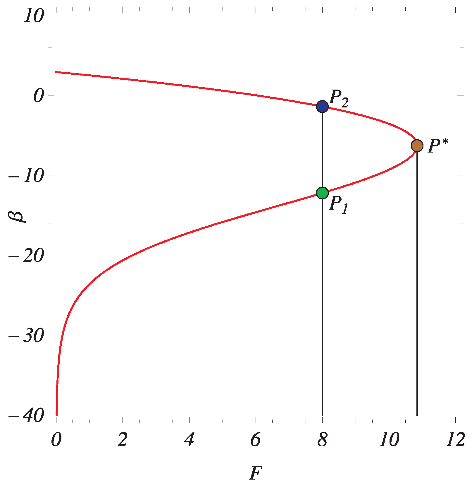
. By numerical analysis, the curve
is ⊃-shaped and has a turning point
from right to left. Thereby, (
11), (
12) has exactly two solutions if
, exactly one solution if
, and has no solutions if
.
In
Figure 2, the bifurcation curve
is depicted for
. The vertical straight line
and the curve
intersect at the points
and
; the point
is a turning point of
. In
Figure 3, three solutions of (
11), (
12) are presented: the green solution corresponds to the point
, the blue solution corresponds to the point
, and the brown solution corresponds to the point
. In
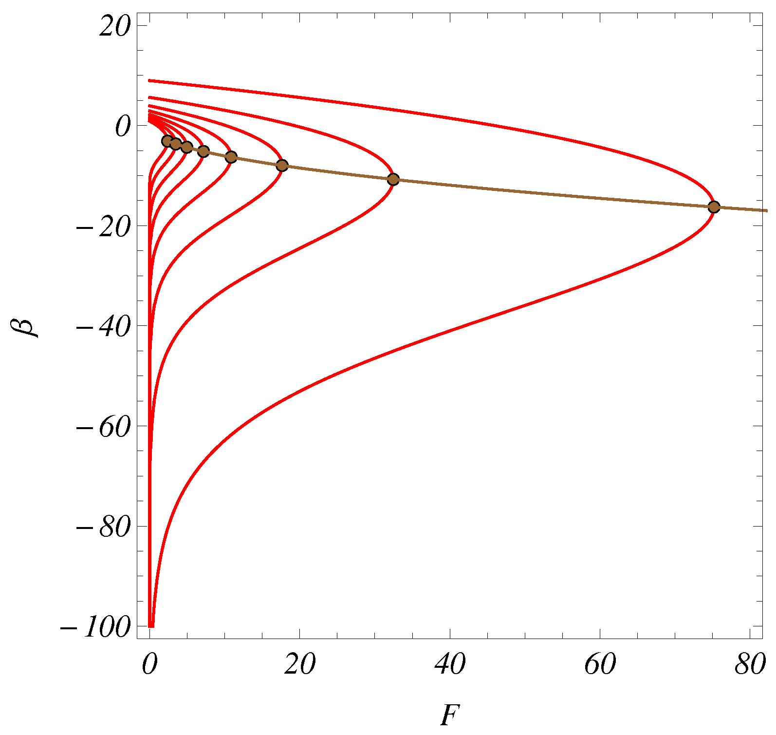
Figure 4, the bifurcations curves
and their turning points are depicted if
,
. In
Figure 5, the dependence of
on
R is presented for
,
, where
is a turning point of
.
4. Linear Stability Analysis
Bifurcation analysis conducted in the previous section allows one to determine (for each
R) the range of values of
F for which there exists a steady solution of (
11) and (
12), namely,
, where
is given by
Figure 5. In addition, it helps to select the base flow temperature distribution (the physically realizable solution is shown in
Figure 3 in blue and has the smallest norm).
Consider a perturbed flow of the form
where
,
k is the wave number, and
is a complex eigenvalue. Base flow (
6) is said to be linearly stable if all
, and linearly unstable, if at least one
. Previous studies [
39] have shown that the most unstable perturbation is axisymmetric for relatively small gaps (including the case
considered in the present paper) so that we restrict ourselves to axisymmetric perturbations. Substituting (
16) into (
2)–(
4) we obtain
The boundary conditions are
Equations (
17), (
18) and (
20) are transformed to one ordinary differential equation of order four by eliminating
q and
w from (
17), (
18) and (
20). The obtained equation is coupled with (
19). In addition, two extra boundary conditions for the function
u are required:
Conditions (
22) follow from (
20) and (
21). The functions
and
for the corresponding boundary value problem are approximated as follows:
where
and
is the Chebyshev polynomial of the first kind. The collocation method is used to discretize the obtained problem where the collocation points are
The discretized generalized eigenvalue problem is solved using Matlab routine
eig.
5. Numerical Results
Calculations are performed for the following two cases: (a) nonzero boundary conditions (
9) for the function
and (b) zero boundary conditions for the temperature
. We refer to cases (a) and (b) in the paper as Case 1 and Case 2, respectively. The values of the Prandtl number that are chosen for calculations (
) correspond to different types of fluids. In particular, gases usually have the Prandtl number of order 0.7. Larger values of the Prandtl number (from 3 to 15) may correspond to biomass slurry that is typically present during the process of energy recovery from wet waste biomass, as is shown in [
40].
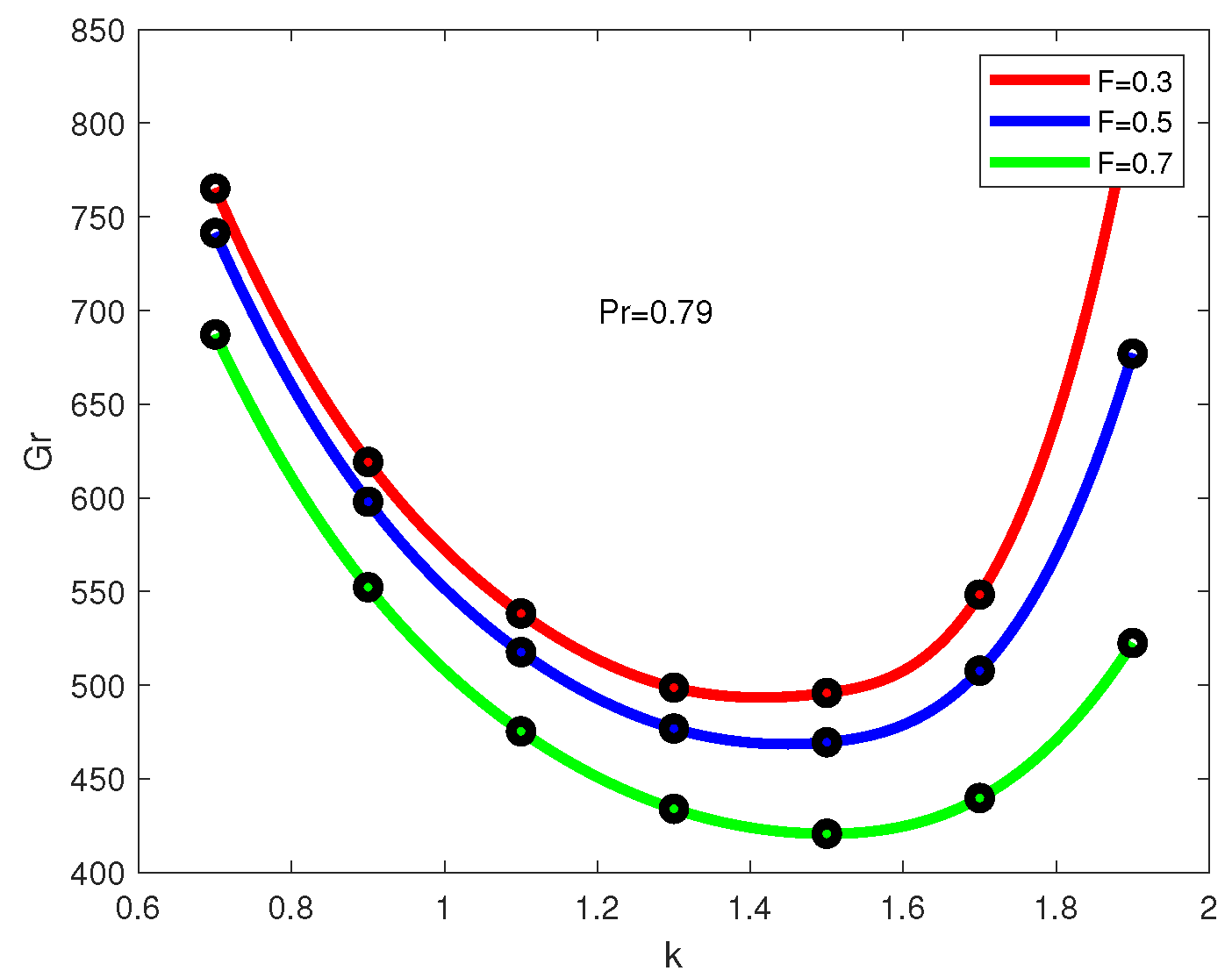
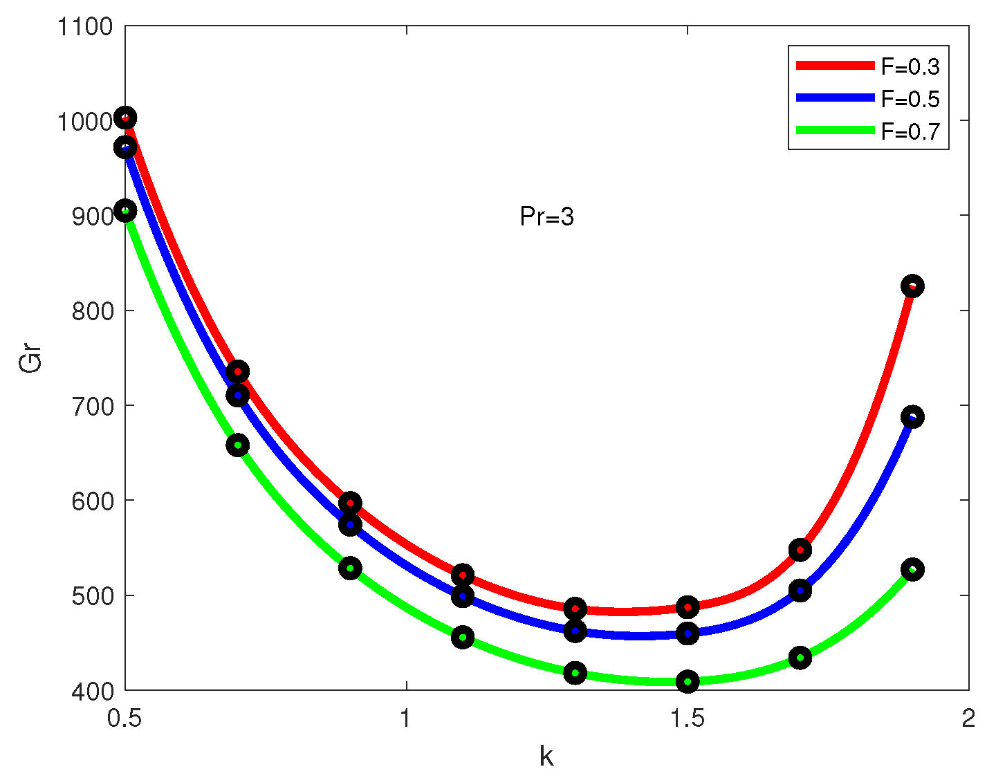
Figure 6,
Figure 7,
Figure 8 and
Figure 9 plot marginal stability curves for four values of the Prandtl number and three values of the Frank-Kamenetskii parameter
F (Case 1 with unequal wall temperatures). The stability region is below the curves.
It can be seen from
Figure 6,
Figure 7,
Figure 8 and
Figure 9 that the increase in
is associated with continuous deformation of the marginal stability curves. For small Prandtl numbers (
and
in
Figure 6 and
Figure 7) all eigenvalues have positive real parts below the curves and negative real parts above the curves, respectively. On the marginal stability curves in
Figure 6 and
Figure 7 one eigenvalue has a zero real part. As the Prandtl number grows, other eigenvalues may become unstable for a certain range of
k while the eigenvalue that was previously unstable may become stable. The appearance of new unstable eigenvalues results in the sharp change of the marginal stability curve and the appearance of additional minima on the marginal stability curves. Note that the second and third minimum appears on the curves for
and
, respectively.
Previous studies [
11,
15,
17,
41] have shown that for large
marginal stability curves can have multiple loops where the base flow is unstable with respect to several modes. Our objective is not to provide detailed description of the marginal stability curves, but to determine the values of the parameters that correspond to the absolute minimum on the marginal stability curve. As a result, we provide only envelopes of the marginal stability curves shown in
Figure 6,
Figure 7,
Figure 8 and
Figure 9.
The critical Grashof numbers
and the corresponding critical wave numbers
are shown in
Figure 14 and
Figure 15, respectively. The “elbows” for the curves in
Figure 14 represent the change of the form of instability (see
Figure 8 and
Figure 9): the minimum that appears in the region of smaller
k as
increases is further lowered as
continues to increase. The second minimum (at
) is not so sensitive to the change in
(see
Figure 8 and
Figure 9). Eventually the two minima coincide: calculations show that for
we have two equal minima (
at
and
). A further increase in
leads to the critical Grashof numbers in the region of smaller
k. As a result, one has a finite jump from
to
(see
Figure 15) and the critical Grashof numbers start to decrease. Similar changes in
and
take place also for
and
. The appearance of the third minimum on the marginal stability curve (see
Figure 9) leads to another jump in
k for the cases
and
.
Critical values of the Grashof number and the corresponding critical wave numbers are shown in
Figure 16 and
Figure 17 for Case 2 (zero wall temperatures). Comparing
Figure 14 and
Figure 15 for Case 1 with the corresponding
Figure 16 and
Figure 17 for Case 2, we see different behavior of the instability modes. The critical values of the Grashof number for Case 2 decrease monotonically as
grows, and the critical wave numbers do not change much in the range of the Prandtl numbers considered:
. In contrast, for Case 1 there is a “plato” phase for each
F where the critical Grashof numbers do not change. Further increase in
leads to a decrease of the critical Grashof numbers.
6. Discussion
Linear stability analysis of a steady convective flow caused by two factors: (a) internal heat generation as the result of a chemical reaction and (b) different constant wall temperatures is analyzed in this paper. The flow is considered in a vertical annular fluid layer under the assumption that the total fluid flux through the cross-section of the layer is equal to zero. The corresponding boundary value problem for the heat equation is nonlinear. Bifurcation analysis is performed in the paper to identify the number of solutions of the boundary value problem depending on the value of the Frank-Kamenetskii parameter, representing the intensity of heat release as a result of the chemical reaction. In addition, solutions to the nonlinear boundary value problem are also obtained. The goal of the bifurcation analysis is to select the correct form of the base flow solution.
The linear stability problem is solved numerically using a collocation method. Two cases are considered separately: Case 1 (different constant wall temperatures) and Case 2 (zero wall temperatures). Calculations show that linear stability characteristics differ considerably between Case 1 and Case 2. In Case 1, multiple minima of the marginal stability curves are observed as the Prandtl number increases. Depending on the relative values of the local minima, the global minimum can be associated with different wave numbers. As a result, finite jumps in wave numbers are observed as the Prandtl number increases. Critical Grashof numbers almost do not change in the interval , where depends on the Frank-Kamenetskii parameter F. In the region the critical Grashof numbers decrease monotonically as the Prandtl number increases. Marginal stability curves for Case 2 have one minimum in the range of the Prandtl numbers considered, , and the corresponding wave numbers do not change much. The results show that instability is mainly of hydrodynamical nature for small Prandtl numbers considered in the paper (). It occurs due to the presence of inflection points in the base flow velocity profile. As the Prandtl number increases, new modes of instability appear; thermal factors are playing a more important role. The appearance of the new modes is seen from the marginal stability curves where one or two additional minima are observed as the Prandtl number grows. Thus, either shear or buoyant instability takes place depending on the value of the Prandtl number.
In order to analyze the development of instability in the region of the parameter space where the flow becomes linearly unstable weakly nonlinear theory can be considered. The approach is based on the use of a multiple scale method where the expansion is constructed in the neighborhood of the critical point
). It is assumed that the Grashof number is slightly above the critical value so that the flow is unstable but the growth rate of the unstable perturbation is small. The result is an amplitude evolution equation for the most unstable mode (such as the complex Ginzburg–Landau Equation [
42]). Weakly nonlinear models were successfully used in the past to investigate instability above the threshold for Taylor–Couette flows [
43] or shallow water flows [
44]. The advantages of the weakly nonlinear method are as follows. First, the amplitude evolution equation is usually much simpler to deal with than the full nonlinear formulation of the problem. Second, some of the amplitude equations can have a rich variety of solutions from deterministic to almost chaotic depending on the values of the parameters [
42]. Third, previous studies have shown that amplitude evolution equations can be successfully used for a rather wide range in the parameter space, even if the multiple scale expansion is considered in a small neighborhood of the critical point. The authors are currently working on this topic.


