Article

Non-Singular Burton–Miller Boundary Element Method for Acoustics

1
Australian Research Council Centre of Excellence for Nanoscale BioPhotonics, School of Science, RMIT University, Melbourne, VIC 3001, Australia
2
Institute of High Performance Computing, Agency for Science, Technology and Research, 1 Fusionopolis Way, Singapore 138632, Singapore
*
Author to whom correspondence should be addressed.
Fluids 2023, 8(2), 56; https://doi.org/10.3390/fluids8020056
Submission received: 1 December 2022 / Revised: 18 January 2023 / Accepted: 1 February 2023 / Published: 5 February 2023

Abstract

:
The problem of non-unique solutions at fictitious frequencies that can appear in the boundary element method for external acoustic phenomena described by the Helmholtz equation is studied. We propose a method to fully desingularise in an analytical way the otherwise hyper-singular Burton–Miller framework, where the original boundary element method and its normal derivative are combined. The method considerably simplifies the use of higher-order elements, for example, quadratic curved surface elements. The concept is validated using the example of scattering on a rigid sphere and a rigid cube, and its robustness and effectiveness for external sound-wave problems are confirmed.

1. Introduction

Understanding acoustic phenomena [1] is of great importance for transitional research and practical applications, ranging from musical instruments [2,3], traffic, or airplane noise prediction [4,5], to sensing and monitoring for structural health [6]. In fluids, acoustic phenomena manifest themselves as the temporal–spatial distribution and evolution of pressure or density waves.
One of the most common acoustic phenomena is sound waves [7] travelling in a fluid at rest, where viscous effects are negligible. Furthermore, assume that the sound wave introduces small perturbations to the fluid density, pressure, and velocity, such that higher-order effects can be ignored. The continuity and momentum equations for linearised acoustic phenomena in a fluid can then be obtained. Meanwhile, under the linearised assumption, the disturbed or fluctuated fluid movement associated with the sound wave is irrotational [8], we can introduce a velocity potential, and the continuity and momentum equations are combined and simplified to become a linear wave equation [9]. The wave equation describing linear acoustics is 2 ϕ = 1 / c 2 2 ϕ / t 2 , with 2 the Laplacian operator, c the speed of sound, t the time, and ϕ the velocity potential. It is usually convenient and intuitive to analyse periodic wave phenomena in the frequency domain, and we have powerful tools based on the Fourier transform to convert wave problems between the time and frequency domains. In the frequency domain, with ϕ ( x , t ) = ϕ ( x ) exp ( i ω t ) , ω being the angular frequency and i = 1 the imaginary unit, the wave equation turns into the scalar Helmholtz equation,
2 ϕ + k 2 ϕ = 0 ,
where k = ω / c is the wave number. The pressure, p, can be obtained from the velocity potential as p = i ω ρ 0 ϕ in the frequency domain, in which ρ 0 is the reference fluid density.
To study sound propagation and scattering in a fluid, we need to solve the Helmholtz equation in Equation (1). Except for a few special cases, such as a spherical or a cylindrical scatterer, it is not feasible to obtain an analytical solution of the Helmholtz equation. Thus, we have to revert to solving the Helmholtz equation numerically and the boundary element method is an effective way to do so [10,11,12,13,14]. The Helmholtz equation (1) is elliptic in nature. Based on Gauss’ theorem and Green’s identities, the boundary element method uses this ellipticity to obtain a relationship between the velocity potential and its normal derivative on the surface of any object or scatterer. Thus, the dimension of the problem can be reduced effectively from a fully three-dimensional (3D) problem to a two-dimensional (2D) surface problem. In addition, the boundary element method is especially advantageous for open space (external) problems, as the Sommerfeld radiation condition [15] at infinity is automatically satisfied and only the surfaces of the objects, S, need to be considered in the meshing. The boundary element method is thus especially suited to solve external problems.
However, a main drawback of external problems when using the boundary element method with large ka values (with a a typical dimension of the problem) is that for certain values of ka, the so-called fictitious wave numbers (or frequencies), the internal resonance solution of the object can appear in the outer solution and, thereby, will produce non-unique (spurious) results. Although it has been shown that it is possible to eliminate certain fictitious frequencies using a modified Green’s function [16], unfortunately, not all fictitious modes can be eliminated in this manner. We have to revert to one of the two most commonly used methods, namely the CHIEF method of Schenck [17] or the method of Burton and Miller [18]. The CHIEF method adds interior points in the internal domain in order to force the internal solution to be zero. The CHIEF method is not entirely rigorous since it is not clearly defined how many and where the internal points should be. In addition, it leads to more equations than variables and a least-square minimisation scheme has to be employed, which can be quite time consuming. The Burton–Miller method, on the other hand, takes the normal derivative of the boundary element equation and adds it to the original boundary element equation. The basic idea is that these two equations always have different fictitious frequencies and it can be shown that, in theory, the combination of these two equations should no longer possess any spurious solutions [19]. The problem with this method is that the integrands now become hypersingular and have to be treated with extreme care [20].
In this paper, the scientific motivation and novelty are to fully desingularise the Burton–Miller formulation, which originally has integrals exhibiting hypersingular integrands. The thus-developed desingularised framework simplifies the numerical implementation considerably since only standard numerical integration schemes are needed. This can greatly increase the opportunity and significantly reduce the threshold to use a technically difficult surface method, the Burton–Miller boundary element method, to solve external acoustic problems robustly, in particular, if one would like to use higher-order surface elements to improve the computational efficiency and accuracy. We demonstrate our method in Section 2 and then validate it in Section 3 using the examples of a rigid sphere and a rigid cube, followed by the conclusion in Section 4.

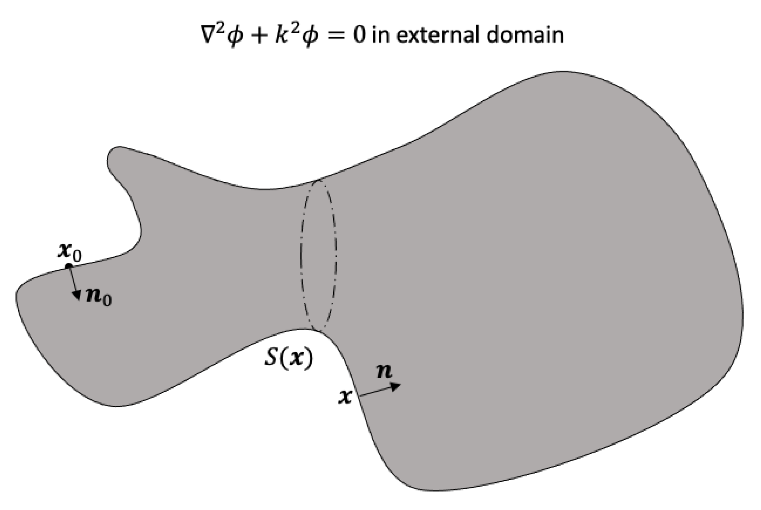
2. The Burton–Miller Framework

2.1. Overview

In this section, we briefly outline the theory of the following sections. We start with the classical boundary integral equation for the Helmholtz equation in Equation (2). The singular integrals can be rewritten as non-singular integrals by subtracting a function satisfying the Laplace equation and using the corresponding Laplace boundary integral method, as demonstrated in Equation (4) in Section 2.2.
In the Burton–Miller framework, we need the normal derivative of the standard Helmholtz boundary integral equation, as in Equation (5). This equation contains hypersingular integrals and must be treated very carefully. It is, however, possible to desingularise it by realising that subtracting the hypersingular kernels of the Helmholtz and Laplace equations results in a weakly singular integrand (see Equation (11)) and using this result in the non-singular Equation (14). This is described in Section 2.3.
Finally, the Burton–Miller idea is to combine the standard boundary integral equation with the normal derivative variant by multiplying by a complex-valued constant β i , as shown in Equation (15). It turns out that we also need to solve an additional boundary integral Equation (16) for a Laplace equation to close the system of equations.

2.2. The Standard Boundary Integral Equation

Given that the Helmholtz equation is elliptic, if the potential and its normal derivative on the surface of the object are given as illustrated in Figure 1, we can obtain all the properties of the acoustic and flow phenomena in the entire fluid domain. However, we normally only know the potential or the normal derivative of the potential (or a linear combination of them) on the surface of the object. To obtain the missing part (see Figure 1 for an example), we can solve the boundary integral equation corresponding to the Helmholtz equation
c ( x 0 ) ϕ ( x 0 ) + S ϕ ( x ) G k n d S ( x ) = S ϕ ( x ) n G k d S ( x ) ,
in which S ( x ) is the surface of the object under consideration, x 0 is the observation point (located on the surface S), c ( x 0 ) is the solid angle at x 0 , x is the integration point, and G k G k ( x 0 , x ) = exp ( i k r ) / r is the Green’s function for the Helmholtz equation, with r = | x x 0 | . The symbol / n = n · represents the normal derivative, where n is the unit normal direction at x pointing out of the domain (thus, into the object).
Suppose we construct a function in the domain of interest as ψ ( x ) = ϕ ( x 0 ) + ( ϕ / n ) 0 n 0 · ( x x 0 ) . Here, ϕ ( x 0 ) is the velocity potential and ( ϕ / n ) 0 is the normal derivative of that potential at x 0 , which are both constants at a given x 0 , and n 0 n ( x 0 ) is the unit normal vector at x 0 on S pointing out of the domain. Clearly, ψ ( x ) is a linear function of x that satisfies the Laplace equation as 2 ψ ( x ) = 0 . The Laplace equation can be taken as a special case of the Helmholtz equation when k = 0, and we can write a similar boundary integral equation for ψ similar to Equation (2) as
[ c ( x 0 ) 4 π ] ϕ ( x 0 ) + S ϕ ( x 0 ) + ϕ n 0 n · ( x x 0 ) G 0 n d S ( x ) = S ϕ n 0 ( n 0 · n ) G 0 d S ( x ) ,
in which G 0 G 0 ( x 0 , x ) = 1 / r is the fundamental solution of the Laplace equation, the normal derivative ψ / n = ( ϕ / n ) 0 ( n 0 · n ) on the surface S has been used, and the term with 4 π is the contribution from the surface at infinity [21,22,23]. Noting that ( n 0 · n ) = 1 in the limit of x x 0 and subtracting Equation (3) from Equation (2), we obtain [24]:
4 π ϕ ( x 0 ) + S ϕ ( x ) G k n ϕ ( x 0 ) G 0 n d S ( x ) = S ϕ n 0 n 0 · ( x x 0 ) G 0 n d S ( x ) + S ϕ ( x ) n G k ϕ n 0 ( n 0 · n ) G 0 d S ( x ) .
The integrands in Equation (4) are now fully regularised.

2.3. The Normal Derivative of the Boundary Integral Equation

We can also perform the normal derivative [ ( · ) / n ] 0 ( · ) / n 0 n 0 · x 0 ( · ) operator on Equation (2), which leads to
c ( x 0 ) ϕ n 0 + S ϕ ( x ) 2 G k n n 0 d S ( x ) = S ϕ ( x ) n G k n 0 d S ( x ) .
The integral on the left is now hypersingular and must be treated with the utmost care when solved directly. In addition, it is worth noting that to obtain the above equation, we have implicitly used [ c ( x 0 ) / n ] 0 = 0 . This is because
c ( x 0 ) + S G 0 n d S ( x ) = 4 π .
Performing the [ ( · ) / n ] 0 operator on the above Equation (6), we have
c ( x 0 ) n 0 + S 2 G 0 n n 0 d S ( x ) = 0 .
Since it has been shown [25,26] that
S 2 G 0 n n 0 d S ( x ) = 0 ,
we conclude that [ c ( x 0 ) / n ] 0 = 0 .
Either Equation (2) or Equation (5) can be used to solve the Helmholtz equation in Equation (1). As we mentioned before, for external problems, both of them suffer from spurious solutions at fictitious frequencies.
Although the traditional Burton–Miller boundary element method based on Equations (2) and (5) eliminates the spurious solutions for external problems, there remain challenges in its numerical implementation due to the singularities as x x 0 when using linear or high-order surface elements, in particular, the hypersingularity. In addition, if we would like to use higher-order surface elements to represent the object, the calculation of the solid angle c ( x 0 ) is tedious. As such, it would be desirable to have a Burton–Miller boundary element method for the Helmholtz equation in which all the singularities and solid angles are fully removed analytically, as demonstrated below.
To handle the main challenge of the integrand on the left-hand side of Equation (5), which is hypersingular as x x 0 , let us define a function ψ 1 that satisfies the Laplace equation instead of the Helmholtz equation and is applied to the same domain and boundaries. Following the same procedure used to obtain Equation (5), we have
c ( x 0 ) ψ 1 n 0 + S ψ 1 ( x ) 2 G 0 n n 0 d S ( x ) = S ψ 1 ( x ) n G 0 n 0 d S ( x ) .
Assuming now that ψ 1 = ϕ on the surface S (and only on this surface), subtract Equation (9) from Equation (5), to obtain
c ( x 0 ) ϕ n 0 c ( x 0 ) ψ 1 n 0 + S ϕ ( x ) 2 G k n n 0 2 G 0 n n 0 d S ( x ) = S ϕ ( x ) n G k n 0 d S ( x ) S ψ 1 ( x ) n G 0 n 0 d S ( x ) .
The integrands in Equation (10) are all weakly singular [27] since (see Appendix A)
lim x x 0 2 G k n n 0 2 G 0 n n 0 = k 2 2 | x x 0 | .
To analytically remove the remaining singularities and the terms associated with the solid angle at x 0 in Equation (10), we set up the following three functions that all satisfy the Laplace equation:
ψ 2 ( x ) = k 2 2 ϕ ( x 0 ) n 0 · ( x x 0 ) ( linear ) , ψ 3 ( x ) = ϕ n 0 ( constant ) , ψ 4 ( x ) = ψ 1 n 0 ( constant ) .
Note that ψ 2 ( x ) is a linear function and ψ 3 ( x ) and ψ 4 ( x ) are constants in the domain, as ϕ ( x 0 ) , ( ϕ / n ) 0 , and ( ψ 1 / n ) 0 are constants for a given x 0 . Following the same procedure used to obtain Equation (3), we can write the boundary integral equations for ψ 2 ( x ) , ψ 3 ( x ) , ψ 4 ( x ) , respectively, as
S k 2 2 ϕ ( x 0 ) n 0 · ( x x 0 ) G 0 n d S ( x ) = S k 2 2 ϕ ( x 0 ) ( n 0 · n ) G 0 d S ( x ) , [ c ( x 0 ) 4 π ] ϕ n 0 + S ϕ n 0 G 0 n d S ( x ) = 0 , [ 4 π c ( x 0 ) ] ψ 1 n 0 S ψ 1 n 0 G 0 n d S ( x ) = 0 ,
in which, ψ 2 ( x ) / n = k 2 ϕ ( x 0 ) n 0 · n / 2 , ψ 3 ( x ) / n = 0 , and ψ 4 ( x ) / n = 0 have been used. Subtracting Equation (13) from Equation (10), we obtain
S ϕ ( x ) 2 G k n n 0 2 G 0 n n 0 k 2 2 ϕ ( x 0 ) n 0 · n G 0 d S ( x ) = S ϕ ( x ) n G k n 0 + ϕ n 0 G 0 n d S ( x ) S ψ 1 ( x ) n G 0 n 0 + ψ 1 n 0 G 0 n d S ( x ) S k 2 2 ϕ ( x 0 ) n 0 · ( x x 0 ) G 0 n d S ( x ) 4 π ϕ n 0 + 4 π ψ 1 n 0 .
The integrands in Equation (14) are now all regular and this equation is fully desingularised. Note that two plus signs appear in this equation since differentiation of r = | x x 0 | with respect to x 0 will produce a minus sign compared to x , that is, x 0 ( r ) = x ( r ) . Here, it is worth noting that we defined ( · ) / n = x ( · ) · n ( x ) and [ ( · ) / n ] 0 = x 0 ( · ) · n ( x 0 ) . For the acoustic flow velocity potential, ϕ / n = x ϕ · n ( x ) and ( ϕ / n ) 0 = x 0 ϕ · n ( x 0 ) refer to the normal velocity at x and x 0 on the boundary, respectively. They are just the normal velocity at different locations by definition such that no minus sign difference will appear here. However, G 0 = 1 / r = 1 / | x x 0 | is the kernel that reflects how some physical property at x will affect that at x 0 or vice versa. Thus, its derivative will depend on the location ( x or x 0 ) we choose as the observation point and the location we choose as the computation point. In this case, there will be a minus sign difference between G 0 / n and G 0 / n 0 with respect to x and x 0 , respectively, since r = | x x 0 | = ( x x 0 ) 2 + ( y y 0 ) 2 + ( z z 0 ) 2 and x 0 ( r ) = x ( r ) = ( x x 0 ) / r .

2.4. The Non-Singular Burton–Miller Formulation

To recover the uniqueness of the solution of the boundary integral method for the Helmholtz equation in the external domain, Burton and Miller proposed to combine Equations (2) and (5) as {Equation (2) + i β Equation (5)} since the fictitious frequencies in Equations (2) and (5) are always different from each other. To balance Equations (2) and (5) in dimension (dimensional homogeneous in length), the parameter β should be related to a characterised length of the problem under consideration. The obvious choices are the size of the scattering object or the inverse of the wave number k.
Following the Burton–Miller concept and combining the non-singular boundary integral equations in Equations (4) and (14), we obtain the non-singular Burton–Miller boundary integral method for the Helmholtz equation as
4 π ϕ ( x 0 ) + S ϕ ( x ) G k n ϕ ( x 0 ) G 0 n d S ( x ) + i β S ϕ ( x ) 2 G k n n 0 2 G 0 n n 0 k 2 2 ϕ ( x 0 ) n 0 · n G 0 d S ( x ) = S ϕ ( x ) n G k ϕ n 0 n 0 · n G 0 d S ( x ) + S ϕ n 0 n 0 · ( x x 0 ) G 0 n d S ( x ) + i β S ϕ ( x ) n G k n 0 + ϕ n 0 G 0 n d S ( x ) i β S ψ 1 ( x ) n G 0 n 0 + ψ 1 n 0 G 0 n d S ( x ) i β S k 2 2 ϕ ( x 0 ) n 0 · ( x x 0 ) G 0 n d S ( x ) i β 4 π ϕ n 0 + i β 4 π ψ 1 n 0 ,
which should be solved simultaneously with the desingularised version of Equation (9):
4 π ϕ ( x 0 ) + S ϕ ( x ) ϕ ( x 0 ) G 0 n d S ( x ) = S ψ 1 ( x ) n ψ 1 n 0 n 0 · n G 0 d S ( x ) + S ψ 1 n 0 n 0 · ( x x 0 ) G 0 n d S ( x ) .
Equation (16) is the non-singular boundary integral formulation similar to Equation (4) to link ψ 1 / n and ψ 1 = ϕ on the surface S.
Equations (15) and (16) are the non-singular versions of the Burton–Miller boundary integrals (which turn into the boundary element method once discretised) to solve the Helmholtz equation for external problems in which all the integrands are regular and all the solid angles are removed analytically. In the numerical procedure, only standard numerical integration schemes, such as Gauss quadrature, are needed to calculate all integrals, which significantly simplifies the numerical implementation.

3. Results

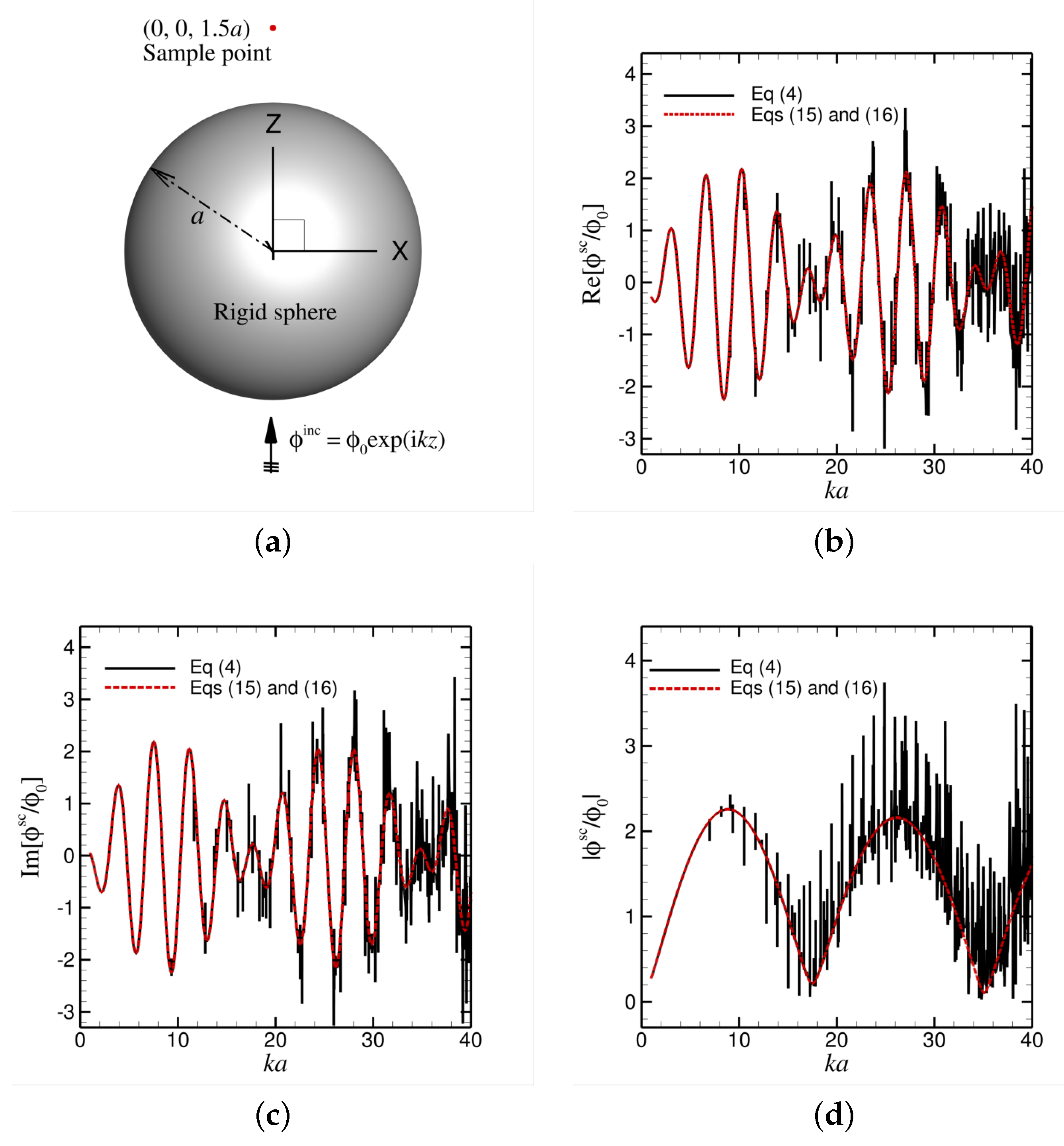
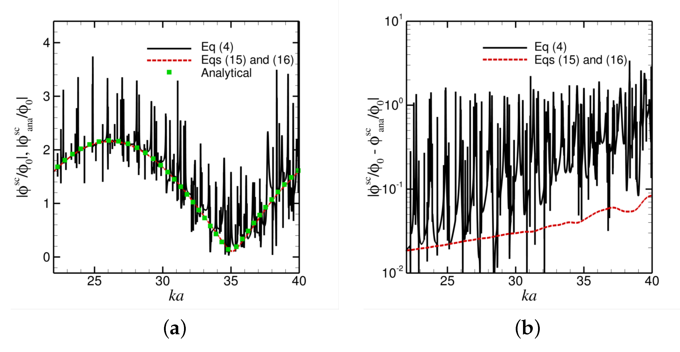
3.1. Scattering from a Rigid Sphere

We test our framework of the non-singular Burton–Miller boundary element method given in Equations (15) and (16) via the classical example of the scattered sound wave by a rigid sphere under an incoming plane wave, as illustrated in Figure 2a. The radius of the rigid sphere is a, and its centre coincides with the origin of the coordinate system. The incoming plane wave moves along the positive z direction with wave number k and amplitude ϕ 0 , whose potential profile can be written as ϕ inc = ϕ 0 exp ( i k z ) . On the surface of the rigid sphere, the boundary condition is that the normal flow velocity is zero, which leads to ϕ inc / n + ϕ sc / n = 0 , where ϕ sc is the potential of the scattered wave.
The scattered sound-wave potential, ϕ sc , is calculated by both the non-singular standard boundary element method, as in Equation (4), and the non-singular Burton–Miller boundary element method, as in Equations (15) and (16), with β = 1 / k when ka spans from 1 to 40 with a step of 0.001. The rigid sphere surface is represented by 5762 nodes connected by 2880 higher-order quadratic triangular elements for all ka values.
We choose the scattered velocity potential at point (0, 0, 1.5a) to serve as the test location to compare the results obtained by those two methods. The procedure to obtain the potential at that location is to solve the scattered potential on the surface of the sphere and obtain the potential in the domain through post-processing [28]. In Figure 2b–d, we show the real part, the imaginary part, and the absolute value of the velocity potential of the scattered wave at the location (0, 0, 1.5a). It is clear that the results obtained by the non-singular standard boundary element method given in Equation (4) are not reliable for high ka values. Non-unique or spurious solutions at fictitious frequencies appear more and more as the value of ka increases, as shown by the spiky black curves in Figure 2b–d. On the contrary, with the non-singular Burton–Miller boundary element method given in Equations (15) and (16), no spurious solutions appear as ka is scanned with a tiny step of 0.001 from ka = 1 up to a high value of 40, as shown by the red curves in Figure 2b–d. Clearly, the non-physical solutions at the classical internal resonance frequencies show up in the curve for the non-singular standard boundary element method, for example, at ka = 9.356 and ka = 10.417, corresponding to the theoretical values of ka = 9.3558 and ka = 10.41712, respectively (see also Table 1 in Ref. [16]).
We also compare the results obtained from the non-singular standard boundary element method of Equation (4) and the non-singular Burton–Miller boundary element method in Equations (15) and (16) with the analytical solution [29] for larger ka ranging from 22 to 40. As shown in Figure 3, the results from the non-singular standard boundary element method are heavily polluted by the spurious solutions, whereas those from the non-singular Burton–Miller boundary element method are in good agreement with the analytical solution for large ka, using a moderate number of surface nodes and higher-order quadratic surface elements.

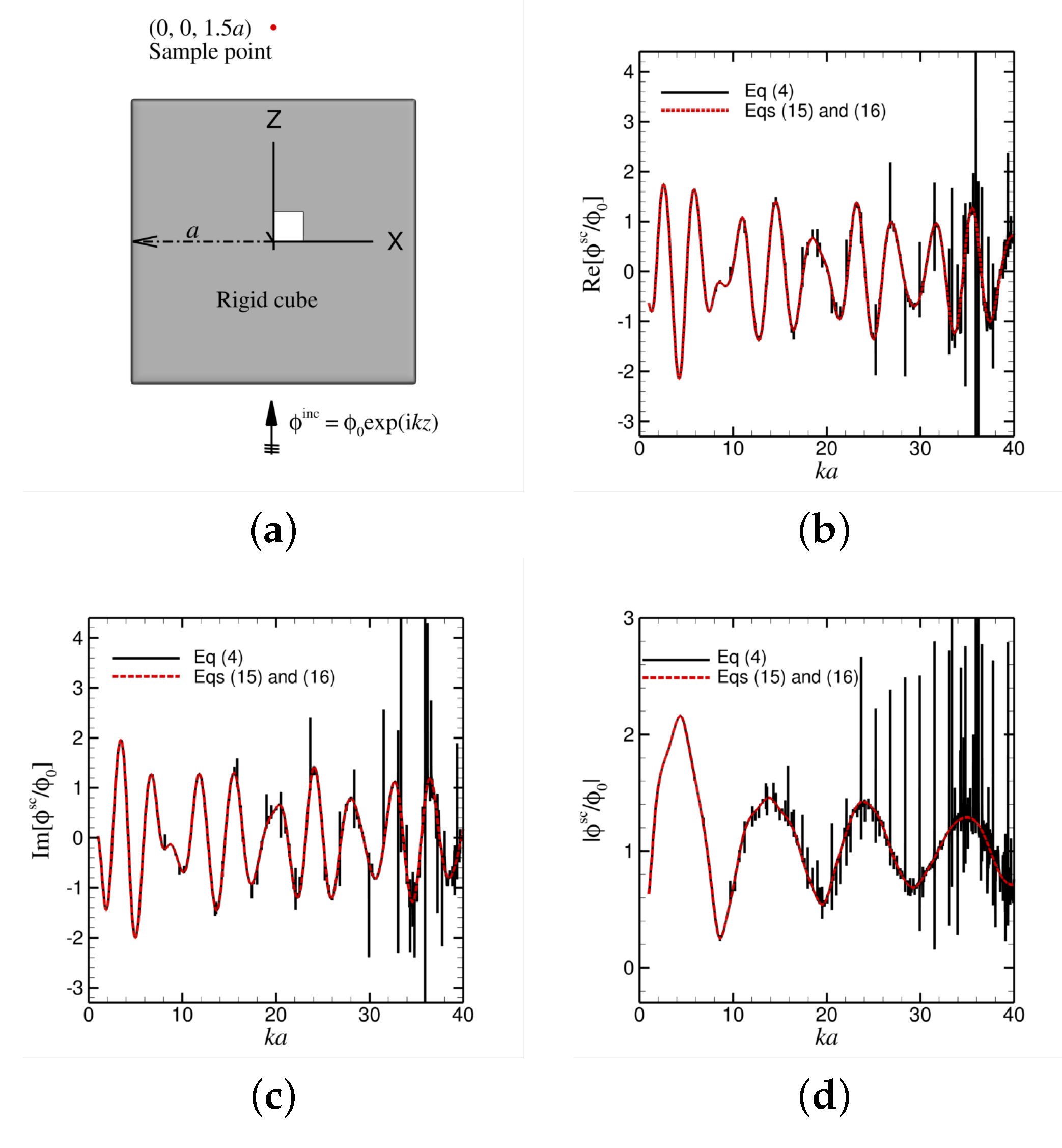
3.2. Scattering from a Rigid Cube

After having performed the verification of a rigid sphere in the previous section, we present a second example of scattering on a rigid cube. As shown in Figure 4a, the cube is aligned with the x-, y-, and z-axes and its centre is situated at (0, 0, 0). The sides of the cube have a length of 2a each and the corners of the cube are rounded in order to facilitate the use of quadratic elements. An incoming wave with wavenumber k travels in the positive z-direction and hits the cube. As in the sphere example, we have placed an observation point at (x, y, z) = (0, 0, 1.5a), thus at a distance of 0.5a behind the cube. In Figure 4b, the normalised real part of the scattered potential ϕ r m s c is plotted as a function of ka, where ka ranges from 1 to 40. The graph was generated by increasing ka in steps of 0.001. As in the previous example, the scattered sound-wave potential, ϕ sc , is obtained with the non-singular standard boundary element method from Equation (4) and the non-singular Burton–Miller boundary element method from Equations (15) and (16), with β = i / k . The cube surface has 11,642 nodes connected by 5820 high-order quadratic triangular elements. As shown in Figure 4b, the red line (Equations (15) and (16)) and the black line (Equation (4)) overlap for up to around ka = 10. For larger values of ka, spurious solutions occur, which are manifested as sharp peaks. A similar trend can be seen in Figure 3c, where the imaginary part of ϕ sc is plotted as a function of ka. It is interesting to note that the peaks that are clearly visible in Figure 4b are not always seen in Figure 4c, and vice versa. Therefore, the absolute value of ϕ sc is also plotted as a function of ka in Figure 4d. The error in the solution for the non-singular standard boundary element method appears to increase with increasing ka, whereas it remains only a few percent for lower ka. However, it can quickly become several times larger, as indicated by the height of the black spikes in Figure 4d.
The observed fictitious frequencies in Figure 4 correspond very closely to the theoretical room-mode formula [29]:
f r o o m = c 2 p 2 L 2 + q 2 W 2 + r 2 H 2
where f r o o m is the frequency where resonance appears in a room with length L, width W, and height H, and p, q, and r are integers 0,1,2 …… Since in our case of a cube, L = 2a, W = 2a, and H = 2a and the relationship between f r o o m and k is f r o o m = k c / ( 2 π ) , we predict that the non-physical solutions might happen at
k a = π 2 p 2 + q 2 + r 2 .
For example, the observed numerical non-physical solution peak at ka = 5.878 corresponds to p = 3, q = 2, and r = 1, with ka = 5.87738, and the numerical non-physical solution peak at ka = 9.683 corresponds to p = 5, q = 3, and r = 2, with ka = 9.68304. It appears that, even with a very small interval of 0.001 for ka, we still missed many of the fictitious frequencies. This confirms the findings of [16,28], where it was found that for moderate ka values, the non-singular boundary element method is already quite good at avoiding non-physical solutions at fictitious frequencies.
The validation examples demonstrated here have shown the robustness and effectiveness of our non-singular Burton–Miller boundary element framework to solve acoustic scattering.

4. Conclusions

In this article, it is shown that it is possible to write the Burton–Miller integral equations in a totally non-singular form. Thus, all elements of the structure can be integrated by standard Gaussian quadrature integration formulas, thereby considerably simplifying the numerical implementation. This ensures that higher-order quadratic meshes can be used with ease to achieve better computational efficiency and accuracy. A further advantage is that solid angles are no longer present in the final integral equations. Such advantages can significantly reduce the threshold to use a technically difficult surface method, the Burton–Miller boundary element method, to solve external acoustic problems robustly and effectively. A slight drawback is that a 2 N × 2 N system must now be solved instead of an N × N system. On the other hand, the use of quadratic elements does allow us to considerably reduce the number of nodes N to achieve the same accuracy compared to flat or linear elements [28]. The concept was tested with two examples, scattering on a rigid sphere and scattering on a rigid cube. The results from the conventional (desingularised) boundary element method and the desingularised Burton–Miller framework were compared for these two examples.
In this paper, we addressed the fictitious frequency issue for sound-wave phenomena described by a scalar Helmholtz equation. However, such issues also appear in vector wave problems, for example, electromagnetic scattering, which in essence, can be considered as three coupled scalar Helmholtz equations—one for each Cartesian component of the electric field [30,31,32,33,34,35] and possibly even for elastic waves [36]. Our framework demonstrated in this paper can also eliminate the non-unique or non-physical solutions at fictitious frequencies in vector wave problems. Furthermore, using Fourier transforms, we can easily extend the method to pulsed phenomena [37]. As such, our framework can be applied to effectively and robustly solve wave phenomena in multi-disciplinary physics.

Author Contributions

Conceptualization, Q.S. and E.K.; methodology, Q.S. and E.K.; software, Q.S.; validation, Q.S.; formal analysis, Q.S. and E.K.; investigation, Q.S. and E.K.; writing—original draft preparation, Q.S. and E.K.; writing—review and editing, Q.S. and E.K.; visualization, Q.S. All authors have read and agreed to the published version of the manuscript.

Funding

This work was partially supported by the Australian Research Council through grants DE150100169, FT160100357, and CE140100003.

Data Availability Statement

The data that supports the findings of this study are available within the article.

Acknowledgments

This research was partially undertaken with the assistance of resources from the National Computational Infrastructure (NCI Australia), an NCRIS enabled capability supported by the Australian Government (Grant No. LE160100051).

Conflicts of Interest

The authors declare no conflict of interest.

Appendix A. Singular Behaviour of the Green’s Functions

The Green’s function for the Laplace equation is G 0 = 1 / r and is thus singular when x x 0 . The normal derivative is G 0 / n = n · ( x x 0 ) / r 3 and appears to be order 1 / r 2 but is actually order 1/r for smooth surfaces since then, the normal vector n is perpendicular to ( x x 0 ) when x x 0 . The second derivative 2 G 0 / n n 0 becomes:
2 G 0 n n 0 = n 0 · n 1 r 3 n · ( x x 0 ) n 0 · ( x x 0 ) 3 r 5
which is hyper-singular with order 1 / r 3 . For the Green’s function of the Helmholtz equation G k = exp ( i k r ) / r , we similarly obtain
2 G k n n 0 = n 0 · n ( 1 i k r ) r 3 e i k r n · ( x x 0 ) n 0 · ( x x 0 ) ( 3 3 i k r k 2 r 2 ) r 5 e i k r
Now, using a Taylor expansion for small r as e i k r 1 + i k r k 2 r 2 / 2 will give ( 1 i k r ) e i k r 1 + k 2 r 2 / 2 and ( 3 3 i k r k 2 r 2 ) e i k r 3 + k 2 r 2 / 2 . Using this and subtracting Equation (A1) from Equation (A2) results in
lim x x 0 2 G k n n 0 2 G 0 n n 0 = k 2 2 | x x 0 | = k 2 2 r .
which is thus of order 1/r and is the proof of Equation (A3).

References

  1. Rienstra, S.W.; Hirschberg, A. An Introduction to Acoustics; Eindhoven University of Technology: Eindhoven, The Netherlands, 2004. [Google Scholar]
  2. von Helmholtz, H. Theorie der Luftschwingungen in Röhren mit Offenen Enden; Verlag von Wilhelm Engelmann: Leipzig, Germany, 1896. [Google Scholar]
  3. Nita, B.G.; Ramanathan, S. Fluids in Music: The Mathematics of Pan’s Flutes. Fluids 2019, 4, 181. [Google Scholar] [CrossRef]
  4. Kadar, H.; Le Bras, S.; Bériot, H.; de Roeck, W.; Desmet, W.; Schram, C. Trailing-edge noise prediction by solving Helmholtz equation with stochastic source term. AIAA J. 2021, 60, 1–20. [Google Scholar] [CrossRef]
  5. Smyk, E.; Markowicz, M. Impact of the Soundproofing in the Cavity of the Synthetic Jet Actuator on the Generated Noise. Fluids 2022, 7, 323. [Google Scholar] [CrossRef]
  6. Kudela, P.; Radzienski, M.; Ostachowicz, W.; Yang, Z. Structural Health Monitoring system based on a concept of Lamb wave focusing by the piezoelectric array. Mech. Syst. Signal Process. 2018, 108, 21–32. [Google Scholar] [CrossRef]
  7. Lighthill, J. Waves in Fluids; Cambridge University Press: Cambridge, UK, 2001. [Google Scholar]
  8. Landau, L.D.; Lifshitz, E.M. Fluid Mechanics, 2nd ed.; Pergamon Press: London, UK, 1987. [Google Scholar]
  9. Rayleigh, R. The Theory of Sound; Macmillan and Co., Ltd.: New York, NY, USA, 1896; Volume 2. [Google Scholar]
  10. Becker, A.A. The Boundary Element Method in Engineering; McGraw-Hill Book Company: London, UK, 1992. [Google Scholar]
  11. Brebbia, C.A.; Walker, S. Boundary Element Techniques In Engineering; Newnes-Butterworths: London, UK, 1980. [Google Scholar]
  12. Amini, S.; Harris, P.J.; Wilton, D.T. Coupled Boundary and Finite Element Methods for the Solution of the Dynamic Fluid-Structure Interaction Problem; Springer: Berlin/Heidelberg, Germany, 1992. [Google Scholar]
  13. Bai, M.R. Application of BEM (boundary element method)-based acoustic holography to radiation analysis of sound sources with arbitrarily shaped geometries. J. Acoust. Soc. Am. 1992, 92, 533–549. [Google Scholar] [CrossRef]
  14. Liu, Y. On the BEM for acoustic wave problems. Eng. Anal. Bound. Elem. 2019, 107, 53–62. [Google Scholar] [CrossRef]
  15. Sommerfeld, A. Die Greensche Funktion der Schwingungsgleichung. Jahresber. Dtsch.-Math.-Ver. 1912, 21, 309–353. [Google Scholar]
  16. Klaseboer, E.; Charlet, F.D.E.; Khoo, B.C.; Sun, Q.; Chan, D.Y.C. Eliminating the fictitious frequency problem in BEM solutions of the external Helmholtz equation. Eng. Anal. Bound. Elem. 2019, 109, 106–116. [Google Scholar] [CrossRef]
  17. Schenck, H.A. Improved integral formulation for acoustic radiation problems. J. Acoust. Soc. Am. 1968, 44, 41–58. [Google Scholar] [CrossRef]
  18. Burton, A.J.; Miller, G.F. The application of integral equation methods to the numerical solution of some exterior boundary-value problems. Proc. R. Soc. A 1971, 323, 201–210. [Google Scholar]
  19. Marburg, S. The Burton and Miller method: Unlocking another mystery of its coupling parameter. J. Comput. Acoust. 2016, 24, 1550016. [Google Scholar] [CrossRef]
  20. Langrenne, C.; Garcia, A.; Bonnet, M. Solving the hypersingular boundary integral equation for the Burton and Miller formulation. J. Acoust. Soc. Am. 2015, 138, 3332. [Google Scholar] [CrossRef] [Green Version]
  21. Klaseboer, E.; Sun, Q.; Chan, D.Y.C. Non-singular boundary integral methods for fluid mechanics applications. J. Fluid Mech. 2012, 696, 468–478. [Google Scholar] [CrossRef]
  22. Sun, Q.; Klaseboer, E.; Chan, D.Y.C. A robust and accurate formulation of molecular and colloidal electrostatics. J. Chem. Phys. 2016, 145, 054106. [Google Scholar] [CrossRef]
  23. Sun, Q.; Klaseboer, E.; Khoo, B.C.; Chan, D.Y. A robust and non-singular formulation of the boundary integral method for the potential problem. Eng. Anal. Bound. Elem. 2014, 43, 117–123. [Google Scholar] [CrossRef]
  24. Klaseboer, E.; Sun, Q. Helmholtz equation and non-singular boundary elements applied to multi-disciplinary physical problems. Commun. Theor. Phys. 2022, 74, 085003. [Google Scholar] [CrossRef]
  25. Meyer, W.; Bell, W.; Zinn, B.; Stallybrass, M. Boundary integral solutions of three dimensional acoustic radiation problems. J. Sound Vib. 1978, 59, 245–262. [Google Scholar] [CrossRef]
  26. Chen, K.; Cheng, J.; Harris, P.J. A new study of the Burton and Miller method for the solution of a 3D Helmholtz problem. IMA J. Appl. Math. 2008, 74, 163–177. [Google Scholar] [CrossRef]
  27. Hwang, W.S. Eliminating the fictitious frequency problem in BEM solutions of the external Helmholtz equation. J. Acoust. Soc. Am. 1997, 101, 3336. [Google Scholar] [CrossRef]
  28. Sun, Q.; Klaseboer, E.; Khoo, B.C.; Chan, D.Y.C. Boundary regularized integral equation formulation of the Helmholtz equation in acoustics. R. Soc. Open Sci. 2015, 2, 140520. [Google Scholar] [CrossRef]
  29. Morse, P. Vibration and Sound, 4th ed.; American Institute of Physics: New York, NY, USA, 1991. [Google Scholar]
  30. Klaseboer, E.; Sun, Q.; Chan, D.Y.C. Non-singular field-only surface integral equations for electromagnetic scattering. IEEE Trans. Antennas Propag. 2017, 65, 972–977. [Google Scholar] [CrossRef]
  31. Sun, Q.; Klaseboer, E.; Chan, D.Y.C. A Robust Multi-Scale Field-Only Formulation of Electromagnetic Scattering. Phys. Rev. B 2017, 95, 045137. [Google Scholar] [CrossRef]
  32. Klaseboer, E.; Sun, Q.; Chan, D.Y.C. A field only integral equation method for time domain scattering of electromagnetic pulses. Appl. Opt. 2017, 56, 9377. [Google Scholar] [CrossRef] [PubMed]
  33. Sun, Q.; Klaseboer, E.; Yuffa, A.J.; Chan, D.Y.C. Field-only surface integral equations: Scattering from a perfect electric conductor. J. Opt. Soc. Am. A 2020, 37, 276–283. [Google Scholar] [CrossRef] [PubMed]
  34. Sun, Q.; Klaseboer, E.; Yuffa, A.J.; Chan, D.Y.C. Field-only surface integral equations: Scattering from a dielectric body. J. Opt. Soc. Am. A 2020, 37, 284–293. [Google Scholar] [CrossRef]
  35. Sun, Q.; Klaseboer, E. A Non-Singular, Field-Only Surface Integral Method for Interactions between Electric and Magnetic Dipoles and Nano-Structures. Annal. Phys. 2022, 534, 2100397. [Google Scholar] [CrossRef]
  36. Klaseboer, E.; Sun, Q. Analytical solution for a vibrating rigid sphere with an elastic shell in an infinite linear elastic medium. Int. J. Solids Struct. 2022, 239, 111448. [Google Scholar] [CrossRef]
  37. Klaseboer, E.; Sepehrirahnama, S.; Chan, D.Y.C. Space-time domain solutions of the wave equation by a non-singular boundary integral method and Fourier transform. J. Acoust. Soc. Am. 2017, 142, 697–707. [Google Scholar] [CrossRef] [Green Version]
Figure 1. Sketch of the 3D object bounded by the closed surface S and surrounded by an infinite external domain. The position vectors x and x 0 are also indicated, together with the normal vectors n and n 0 , which are pointing out of the external domain.
Fluids 08 00056 g001
Figure 2. Scattering on a rigid sphere with radius a used as a test case. (a) The incoming plane wave moves upwards and the observation point is behind the sphere at a distance of 1.5 a from the centre of the sphere. (b) The results of the real part of the potential ϕ sc with the non-singular Burton–Miller formulation (in red) as a function of ka. The results of the non-singular standard boundary element method are also indicated (in black); 5762 nodes with 2880 quadratic triangular elements were used. (c,d): as (b) but for the imaginary part of ϕ sc and the absolute value of ϕ sc , respectively.
Fluids 08 00056 g002
Figure 3. As in Figure 2, the spherical test case for ka = 22 to 40. (a) Scaled results of the scattered potential with the non-singular standard boundary element method (in black), the desingularised Burton–Miller framework (red line), and the analytical solution (in green). (b) Error between the analytical result and the non-singular standard boundary element method (black line) and the desingularised Burton–Miller framework (red line).
Fluids 08 00056 g003
Figure 4. Scattering on a rigid cube with sides of length 2a used as a test case. (a) The incoming plane wave moves upwards and the observation point is behind the cube at a distance of 1.5a from the centre of the cube. (b) The results of the real part of the potential ϕ sc , with the non-singular Burton–Miller formulation (in red) as a function of ka. The results of the non-singular standard boundary element method are also indicated (in black). More and more spurious ‘spikes’ appear when ka becomes larger and larger. The number of nodes used is 11,642 with 5820 quadratic triangular elements. (c,d): as (b) but for the imaginary part of ϕ sc and the absolute value of ϕ sc , respectively. As in Figure 2, the desingularized Burton–Miller results (red curves) are perfectly regular for all values of ka.
Fluids 08 00056 g004
Disclaimer/Publisher’s Note: The statements, opinions and data contained in all publications are solely those of the individual author(s) and contributor(s) and not of MDPI and/or the editor(s). MDPI and/or the editor(s) disclaim responsibility for any injury to people or property resulting from any ideas, methods, instructions or products referred to in the content.

